Leaders of neuronal cultures in a quorum percolation model

Introduction

Development of connectivity in a neuronal network is strongly dependent upon the environment in which the network grows: cultures grown in a dish will develop very differently from networks formed in the brain. In a dish, the only signals that neurons are exposed to are chemicals secreted by neighboring neurons, which then must diffuse to other neurons via the large volume of fluid that surrounds the culture. The result is a connectivity dominated by proximity in a planar geometry, whose input degree follows a statistical distribution function that is Gaussian-like (Soriano et al., 2008). This is contrasted by the intricate guidance of axons during the creation of connectivity in the brain, which is dictated by a detailed and very complex “blueprint” for connectivity. As a result, the firing pattern of a culture is an all-or-none event, a population spike in which practically all the neurons participate and are simultaneously active for a brief period of time, spiking about three to four times on average.

We have previously shown (Cohen et al., 2010) that graph theory and statistical mechanics are useful in unraveling properties of the network in a rat hippocampal culture, mostly because of the statistical nature of the connectivity. With these tools we have been able to understand such phenomena as the degree distribution of input connections, the ratio of inhibitory to excitatory neurons and the input cluster size distribution (Breskin et al., 2006; Soriano et al., 2008). We found that a Gaussian degree distribution gives a good quantitative description for statistical properties of the network such as the appearance of the giant m-connected component and its size as a function of connectivity. The inhibitory component was found to be about 30% in hippocampal cultures, and about 20% in cortex. We furthermore observed that the appearance of a fully connected network coincides precisely with the time of birth (Soriano et al., 2008).

In this paper we apply our graph theoretic approach to the intriguing process of the initiation of a spontaneous population spike. On the one hand, a perturbation needs to be created that pushes a number of neurons to begin firing. On the other hand, the initial firing pattern must propagate to the rest of the neurons in the culture. Understanding this recruitment process will give insight on the structure of the network, on the interrelation of activation in neurons, and on the dynamics of neuronal firing in such a complex culture. A simple scenario for initiation that one might conceive of is wave-front propagation, in which a localized and limited area of initiation is ignited first, and from there sets up a spherical traveling front of excitation. However, as we shall see, the initiation is a more intricate process.

The experimental situation regarding initiation of activity is complex. In quasi one-dimensional (1D) networks we have been able to show that activity originates in a single “Burst Initiation Zone” (BIZ), in which a slow recruitment process occurs over several hundreds of milliseconds (Golomb and Ermentrout, 1999, 2002; Osan and Ermentrout, 2002; Feinerman et al., 2005). From this BIZ the activity propagates to the rest of the linear culture along an orderly and causal path dictated by the 1D structure (Feinerman et al., 2007). In 2D networks such causal propagation is not observed (Maeda et al., 1995; Streit et al., 2001), and the precise mode of propagation has not been identified. Recently, Eytan and Marom (2006) found that a small subgroup of neurons were the “first-to-fire,” and that also in this case the initiation is long (on the order of hundreds of milliseconds). They also observed that the growth rate is exponential in the initial stage and then changes to faster than exponential. These neurons were later shown to characterize and “lead” the burst, and to recruit the neurons in their proximity in the “pre-burst” period (Eckmann et al., 2008).

In this paper we address and connect three experimental observations that are at first sight unrelated. The first and fundamental observation is the fact that bursts are initiated by Leaders, or first-to-fire neurons (Eytan and Marom, 2006). We use the quorum percolation model to answer the question – what makes these Leaders different from the rest of the network – by showing that one of their important characteristics is a high in-degree, i.e., a large number of input connections.

We then turn to the second experimental observation, that the activity in a burst starts with an exponential growth. We show that this can happen only if the distribution of in-degree is a power law with exponent of −2. However, this needs to be related with the third experimental observation, which is that the distribution of in-degrees is Gaussian rather than power law. We reconcile both observations by stitching together the two solutions into an in-degree distribution that has the large majority of neurons in a Gaussian centered around an average in-degree of about 75, while 10% of the population lie on a power law tail that can reach a few thousand connections. We show that this reconstructs the full experimentally observed burst structure, which is an exponential initiation during the pre-burst followed by a super-exponential during the burst.

We present several ideas on the origin of these distributions in the spatial extent and geometry of the neurons, and show that the distribution of in-degrees is proportional to the distribution of spatial sizes of the dendritic trees. We thus conjecture that the distribution of dendritic trees is mostly Gaussian, but that a few neurons must have dendrites that go off very far, with power law distribution of this tail. We end by making some additional conjectures about 1D cultures and on the importance of the size of the culture.

Methods

Quorum Percolation Model for Dynamics of Random Graph Network

We describe the neural culture using a simplified model of a network whose nodes are neurons with links that are the axon/dendrite connections. This picture is further simplified if we consider a randomly connected sparse graph (Bollobas, 1998), with a uniform strength on all the connections. The structure and topology of the graph are determined by specifying a probability distribution p_k for a node to have k inputs. Percolation on a graph is the process by which a property spreads through a sizeable fraction of the graph. In our case, this property is the firing of neurons. The additional characteristic of Quorum Percolation is, as its name implies, that a burst of firing activity will propagate throughout the neuronal culture only if a quorum of more than m firing neighbors has ignited on the corresponding graph. While this description makes a number of assumptions that are not exact in their comparison to the experiment, it does, as we have been able to show previously, capture the essential behavior of the network (Tlusty and Eckmann, 2009; Cohen et al., 2010). The use of such a simple model for the neuronal network is justified at the end of the Section “Methods.”

In particular, in this paper we obtain a theoretical explanation for the experimental observation of initiation of activity by a small number of neurons from the network and the subsequent gradual recruitment of the rest of the network. Within the framework of a random graph description, we have previously shown that the dynamics of firing in the network is described by a fixed point equation for the probability of firing in the network, which also corresponds to the experimentally observed fraction of neurons that fire. Experimentally, this fraction can be set by applying an external voltage (Breskin et al., 2006; Soriano et al., 2008). In the case of spontaneous activity, this fraction is determined by the interplay of noise and the intrinsic sensitivity of the neurons (Alvarez-Lacalle and Moses, 2009).

Specifically, connections are described by the adjacency matrix A, produced according to the probability distribution p_k, with A_ij = 1 if there is a directed link from j to i, and A_ij = 0 otherwise and A_ii = 0.

Our study starts by assuming initial conditions where a fraction f of neurons are switched “on” externally at time t = 0. The neurons fire, and once they do they stay “on” forever – a neuron will be on at time t + 1 if at time t it was on. A neuron is either turned on at t = 0 (with probability f) or, if it is off at time t, then it will it will be turned on at time t + 1 if at least m of its upstream (incoming) nodes were on at time t:

where s_i(t) describes the state of the neuron at time t (1 for “on” and 0 for “off”) and Θ is the step function (1 for x ≥ 0, 0 otherwise). Note that the second term, which accounts for the neuron’s probability to fire at time step t, creates a coupling of s_i(t) to all its inputs s_j(t). Lacking a turning off process, the number of active nodes is monotonically increasing and converges into a steady state (a fixed point) within a finite time t_f, which is smaller than the number of neurons, t_f < N.

To derive the “mean-field” dynamics for the average fraction of firing neurons, Φ(t) = 〈s_i(t)〉 = N⁻¹Σ_is_i(t), one cannot simply average Eq. 1 directly. This is due to the correlation between s_i(t) and Θ (Σ_jA_ijs_j(t) − m). The correlation exists because if a given neuron fires, s_i(t) = 1, and it was not externally excited, then at least m of its inputs are firing and the step function over its inputs must also be 1. In fact, at the fixed point the correlation is strong, (1 − s_i(t)) Θ (Σ_jA_ijs_j(t) − m) = 0, since in the steady state a neuron can remain off if and only if less than m of its inputs fire. To avoid the correlations, one utilizes the monotonicity to realize that a neuron is on only if it was turned on externally at time t = 0 or, if it was off at t = 0 then at some time t at least m of its inputs fired. We can then replace s_i(t) by s_i(0) and rewrite Eq. 1 as s_i(t + 1) = s_i 0) + (1 − s_i(0)) Θ (Σ_jA_ijs_j(t) − m). In the tree approximation, which disregards loop feedbacks, the initial firing state of a neuron, s_i(0), cannot affect its inputs, s_j(t). Inversely, it is obvious that s_i(0) which is determined externally is independent of s_j(t). Therefore, s_i(0) and Θ(Σ_jA_ijs_j(t) − m) can be averaged independently. The result is the mean-field iteration map:

where the combinatorial expression for Ψ is the probability that at least m inputs are firing and f is the initial firing fraction, f = Φ(0) = 〈s_i(0)〉. The steady state of the network is defined by the fixed point Φ_∞, which is found by inserting Φ(t + 1) = Φ(t) = Φ_∞ into Eq. 2, to obtain Φ_∞ = f + (1 − f)Ψ(m, Φ_∞).

Collectivity and the Critical Point

The role of Leader neurons in the initiation and the development of bursts can be clarified by dividing the neurons into classes of in-degree k (“k-class”) and looking at the dynamics of each class separately. The total firing probability Φ = Σ_kp_kΦ_k is thus composed of the sum over the individual probabilities Φ_k for each k-class to fire. The mean-field equation for a given k-class is

where Ψ_k is the probability that a neuron with k inputs has at least m that are firing. Although all k-classes are coupled through the common Φ, the formulation of Eq. 3 allows the tracing of the fraction Φ_k of each class and its dynamics during its evolution.

It follows from Eq. 3 that at the fixed point Φ_k,∞ = f + (1 − f)Ψ_k(m, Φ_∞). Given the time dependence of Φ(t), one can extract the fraction of firing neurons in each k-class, Ψ_k, by plugging Φ(t) into Eq. 3.

The combinatorial expressions for Ψ and Ψ_k are:

There is a particular critical initial firing where the solution jumps from Φ ≈ f (i.e., practically all activation is externally driven and there is almost no collectivity, Ψ ≪ 1) to Φ ≈ 1 where most firing is due to inputs (and Ψ ≃ 1). It is both convenient and instructive to treat and simulate the network near this transition point, since the dynamics there is slow. This allows the different steps in the recruitment process to be easily identified and distinguished.

Simulation of the Quorum Percolation Model

The model was numerically investigated by performing a simulation, employing N = 500,000 neurons. This number was chosen to match as close as possible the number of neurons typically in an experiment, which is on the order of one million. An initial fraction f of the neurons were randomly selected and set to “on” (i.e., fired). At every time step a neuron would fire if it fired the previous step, or if more than a threshold number of its input neighbors fired. The threshold m and the initial firing component f could be varied, and the activity history of all neurons was stored for subsequent analysis. We used a number of different degree distributions, including a Gaussian, exponential and power law for the network. We also used a tailored Gaussian distribution in which 10% of the high-k neurons, which have k higher than a given k_tail, obey a power law distribution function.

Validity of the Model

The use of a random graph for neuronal cultures

The spatial extent and arrangement of connections can be of importance to the dynamics of the network. In contrast to spatially embedded (metric) graphs, random graphs allow any two nodes to connect, i.e., they are the analog of infinite dimensional networks. The experiment is obviously metric but our model employs a random graph. This seeming contradiction was resolved in a previous study (Tlusty and Eckmann, 2009), where we showed that if the average connectivity is high enough then the graph is effectively random (i.e., of very high dimension). Why does the random graph picture describe so successfully the measurements of a 2D neural culture while it completely neglects the notions of space and vicinity? As we explained in Tlusty and Eckmann (2009), there is a basic difference in the manner in which random and metric graphs are ignited. In metric graphs it suffices to initially turn on localized excitation nuclei, which are then able to spread an excitation front throughout the spatially extended network. In random graphs, there are no such nuclei and one has to excite a finite fraction of the neurons to keep the ignition going. Still, we showed (Tlusty and Eckmann, 2009) that the experimental network, which is obviously an example of a metric graph, is effectively random, since its finite size and the demand for a large quorum of firing inputs makes the occurrence of excitation nuclei very improbable. As explained in that paper, this occurs when it becomes impossible to identify causal paths in space along which activity propagates, with one neuron activating its neighbor and so on. In other words, the activity burst does not initiate at one specific nucleating site, and has instead multiple locations at which activity appears. This is exactly the characteristic of a random graph with no spatial correlations. Thus a highly connected graph in 2D such as ours has characteristics that are similar to a high dimensional graph with near-neighbor connectivity.

Approximating neuronal cultures as tree-like graphs

The basic reason why a tree-like graph will describe the experimental network lies in the observation that the percentage of connections emanating from a neuron that actually participate in a loop is small. Indeed, we have demonstrated in Soriano et al. (2008) that the average number of connections per neuron is large, about 100. On the other hand, because the network is built from dissociated neurons, the connectivity is determined by a spatial search process during their growth, which is for all practical purposes a random one. We therefore have a random network (embedded in a metric space) with about 100 connections per node.

Such networks do indeed have some loops, and thus we need to study the effect of such loops on the general argument of Eq. 2. For this, it suffices to study the case of 2-loops (which in fact cause the strongest correlations). Assume neuron A and neuron B are linked in a 2-loop.

If neuron A fires at time t then it does not change any more, and therefore the state of B at time t + 1 does not matter for the state of A at any later time. If A is not firing at time t then it decreases the probability of B to fire at time t + 1, and this in turn reduces its own probability to fire at time t + 2. Clearly, this effectively decreases the probability of A to fire. We shall now show that this effect is 1/(k²N) where k is the mean degree (100) and N is the total number of neurons that B can connect to.

To see this, we note that if A is off then the number of available inputs that can fire into B reduces by one, from k to k − 1. We show below that this corresponds changing the ignition level Φ from m/k to m/(k − 1). The overall effect of a 2-loop on the probability of B to fire therefore scales like m/(k − 1) − m/k ≃ m/k². The back-propagated effect on A will be of order m²/k⁴.

To estimate the total number of 2-loops that include neuron A we first look at all trajectories of length 2 that emanate from A. There are such trajectories. Of these a fraction of k_in/N will return to A. The total number of 2-loops that start at A is thus The fraction of inputs of A that participate in a 2-loop is therefore

Assuming that for a typical neuron k_in is equal to k_out, the total effect of 2-loops on Φ calculated at neuron A is therefore m²k²/N/k⁴ = m²/(k²N).

Below we show the applicability of the tree-like random graph model by comparing its results directly to the simulation that uses N = 500,000 neurons. The correspondence between model and simulations (Figures 4 and 5) is satisfactory.

In the experimental case, spatial proximity may lead to more connections than in a random graph. The effect of space is to change the relevant number of neurons N from the total number to those that are actually accessible in 2D. That number N is on the order of N_space = 3,000 as compared to N_total = 500,000. However, 1/k²N is still a small number.

In a separate work, a simulation that takes space into account was performed (Zbinden, 2010), and the number of loops could be evaluated directly. Indeed we found that the number of loops is enhanced over the random graph estimation by a factor of N_space/N_total, but still remains small.

Applicability of the averaged equation (mean-field) approach

In a physical model one must be sure that the ensemble of random examples chosen to average over a given quantity does indeed represent well the statistics of the system that is being treated. In our model, the connectivity of the graph is fixed (“quenched” disorder), and the ensemble is that of the random graphs that can be generated with the particular choice of input connection distribution function. In reality, the experiment and the simulation measure the bursts inside one particular realization. However, the mean-field equation averages over a whole ensemble of such random graphs. The question is whether the averages obtained using one real graph are representative of the whole ensemble. This is a behavior which is termed “self-averaging,” and means that, in the limit of large graphs, one single configuration represents the average behavior of the ensemble.

The similar ensemble of the classic Hopfield (spin-glass) model for neural networks is known to be self-averaging in the limit of an infinite sized graph (van Hemmen, 1982; Provost and Vallee, 1983; Amit et al., 1985). This occurs because the dynamics is performed over a huge number of single neuron excitations.

In practice, our model differs from the neural network model of Amit et al. (1985) in that the neurons of our model change only from “off” to “on,” and cannot flip in both directions as the equivalent “spins” do. We therefore tested numerically the self-averaging property of the graph, and found that it indeed exists for the random graphs we considered, i.e., the fluctuations between specific different realizations of the graph are negligible (see Figure 4 below).

The model describes initial growth of activity

The possibility of turning a neuron “off” is not incorporated in the model because we only consider short times. The whole process described by the simulation occurs over a very brief period of time, and therefore a firing neuron keeps its effect on other neurons during the whole process. To be concrete, the unit of time in the model and in the numerical simulations is the firing of one spike, equivalent in the experiment to about 1 ms. The simulation extends to about 50 units, i.e., describes a process that occurs typically for 50 ms.

In our model a neuron has no internal structure, so that whether it is “on” or “off” impacts only the neurons that are its neighbors. The relevant issue is therefore – how long is the effect of a neuron’s activity felt by its “typical” neighbor. The experimental facts are that a neuron fires on average 4–5 spikes per burst, each lasting a millisecond, with about 4–5 ms between the spikes (Jacobi and Moses, 2007) so that its total active time spans typically 20 ms.

The post-synaptic neuron retains the input from these spikes over a time scale set by the membrane decay constant, which is on the order of 20–30 ms. Therefore, after a firing period of about 20 ms, there is a retention period of comparable duration. We can conclude that the effect of a neuron that has fired can be felt by its neighbors for the total build-up time of the burst, about 50 ms. We therefore describe by “on” the long term, averaged effect of the neuron once it has begun firing. One caveat to this is that the strength of that effect may vary with time, and such an effect is not described within the model.

We also assume, for simplicity, that all the neurons are available and can participate in the burst (no refractive neurons). In the experiment this is equivalent to looking at those bursts that have quiescent periods before them, which is often the case.

The role of inhibitory neurons

In this model all neurons are excitatory; within the “0” or “1” structure of the model, the contribution of an inhibitory neuron would be “−1.” Thus adding inhibitory neurons amounts to increasing m, the number of inputs that must fire before a neuron will fire. This is a small accommodation of the model, and does not change the dynamics of burst initiation.

Below we also model the dynamics of burst activation observed in the experiments of Eytan and Marom (2006), which measured an exponential recruitment at the initial stage of the burst. These experiments clearly show that the dynamics are essentially the same for cultures both with and without inhibition. Both display an initial exponential growth followed by a super-exponent. One small difference lies in the value of the growth, which is larger for dis-inhibited than for untreated cultures. But the main difference is seen only after the burst reaches its peak, in the decay of the burst.

The role of noise in burst initiation

We assume the existence of spontaneous sporadic activity of single neurons in the culture. In principle, this can be treated as a background noise (Alvarez-Lacalle and Moses, 2009). In our case we require that a minimal amount f of the culture spontaneously fires, and we look at the ability of this fraction of initially firing neurons to initiate a burst. It is possible to initiate the activity with an external voltage V, using bath electrodes, as we reported in previous work (Breskin et al., 2006; Soriano et al., 2008). In that case f(V) is determined by the percentage of neurons that are sensitive enough to fire at a voltage V.

Results

First-to-Fire Neurons Lead Bursts and have Large Input Degree

We use the simulation for an initial look at the recruitment process and to identify those neurons that fire first. We use a Gaussian distribution to describe the experimental situation as closely as possible, and put the system near criticality, i.e., with f barely above to observe a large range of changes in activity. Figure 1 shows the degree values k of the neurons as a function of the time step at which they first fire. It is evident that the neurons that fire first are either the ones that were ignited externally or those with high k. This is verified in the lower part of Figure 1, in which we plot, for each neuron, its time of ignition as a function of its in-degree k. It is obvious that the high-k neurons totally dominate the initial stages of the activity.

FIGURE 1

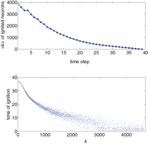
Figure 1. Top: Average k of all neurons ignited at each time step t from one particular realization of the simulation. Bottom: Times of ignition for all 500,000 individual neurons. It is evident that highly connected neurons are the first-to-fire. For clarity we plot time only from t = 1 and do not show the ∼1,000 neurons that were initially ignited at t = 0. We used here f = 0.0033 and p_k which for k < k_tail is a Gaussian centered on with width σ = 31 and is a power law p_k ∼ k⁻² for k > k_tail. We checked that a simple Gaussian p_k gives the same qualitative results.

Further information on the distribution of ignition times for different neurons with different in-degree k is given in the colored map format of Figure 2. The huge majority of neurons has a low k and ignites very late in the burst. The first-to-fire neurons, or Leaders, are few and have a wider distribution of in-degree k at a given time step t. The distribution sharpens as the burst advances in time.

FIGURE 2

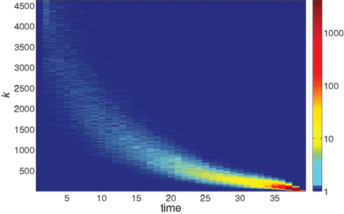
Figure 2. The logarithmic color coding of the number of neurons with in-degree k that ignited at time step t. The data are the same as in Figure 1.

To understand this from the model, we concentrate on the neurons within a given k-class, i.e., the group of neurons with k inputs, and examine the probability of a neuron within this group to fire, Φ_k. If the average number of inputs k¯ and the threshold value m are large numbers, then we can neglect the width of the binomial distribution and approximate the error function Ψ_k(m, Φ) by its limit Θ(k − m/Φ). This simplifies the dynamics Eq. 3 into:

meaning that under this approximation the whole k-class fires once Φ(t) exceeds m/k. In other words, the k-classes are ignited in steps where in each step the classes whose k is in the range m/Φ(t) < k < m/Φ(t − 1) are ignited. Obviously, the first nodes to be ignited are those with the high k. By summation, one finds the iterative equation:

where is the cumulative distribution. The dynamics of the approach to the fixed point can be graphically described as the iterations between the curves Φ and f + (1 − f)P(m/Φ(t)).

The time continuous version of the iteration equation is

which can be integrated, at least numerically, to obtain the dynamics of the system. Within this approximation, the k-class firing is given by the step function Eq. 5. For simple collectivity functions, Ψ, and simple degree distribution p_k Eq. 7 can be integrated analytically. In more complicated cases, an iterative scheme, as detailed in Section “Excitation-Dependent Threshold” below, is needed.

Since these neurons are highly connected, they will statistically be connected to each other as well. For the experimentally relevant case of a Gaussian distribution peaked at 78 connections with a width of 25 (Breskin et al., 2006; Soriano et al., 2008), more than 10% of the neurons have over 100 connections, while about 1% of the neurons have 120 connections or more. Since high-k neurons have more inputs and hence a larger probability to receive inputs from other high-k neurons, these highly connected neurons form an interconnected subgraph. We summarize our understanding by stating that Leaders are highly interconnected, homogeneously distributed and form a sparse sub-network.

In the Multi Electrode Array experiment about 60 neurons were monitored, and a burst was observed to begin with one or two of these neurons. From these initial sites the activity spread. Identifying these neurons as Leaders, we reach the conclusion that in every experimentally accessible patch of the network that we monitor there is a small number of neurons that lead the other neurons in activation. We therefore deduce from the theory that they are part of this highly interconnected, sparse sub-network. In the initial pre-burst period nearby neurons are recruited by inputs from the Leaders, while in the burst itself all the neurons fire together. During the pre-burst a spatial correlation to the Leader exists in its near vicinity, which vanishes as the activity transits to the burst.

We remark here that within our model a node that fires early is highly connected. However, the number of connections k and the threshold for firing m are two factors with the same effect, and they could in fact interplay to cause a more complex behavior than we are describing (Zbinden, 2010). One alternative model could hold the number of connections fixed for all neurons, and only allow a variation in the number of inputs needed for a neuron to fire m. This would clearly bring about a variety of response times of neurons, and could create a subgroup of nodes that fire early. If we allow a few neurons to have a low threshold m then those neurons will qualify as our Leaders. While there is no evidence to point to a wide variability in the threshold of the neurons, there are clear arguments why some neurons may change their threshold in response to the activity of other neurons, either reducing the sensitivity (adaptation) or increasing it (facilitation). In Section “Excitation-Dependent Threshold” we discuss such a possibility, giving a demonstration of how such a scenario could evolve.

Deducing the Connection Distribution from the Initial Growth Rates

The experimentally relevant case of an exponential pre-burst

If the firing order of the neurons is determined by their connectivity, then by observing and analyzing the evolution of the burst we may learn about the connectivity of the neurons. We focus on the experimental fact that the growth rate of the very first firing is exponential, which leads us in the next sections to analyze a particular form of the degree distribution that can lead to exponential growth dynamics.

Our observation that the initial growth of the burst is totally dependent on nodes at the very high-k side of the degree distribution gives an opportunity to find the origin of the initial exponential growth A(t) = e^αt observed by Eytan and Marom (2006). This regime appears at the very beginning of the burst (i.e., at the pre-burst defined in Eckmann et al., 2008), and ends when the majority of the network begins to be active and the actual burst (also defined in Eckmann et al., 2008) occurs. During this period the amplitude of activity A(t) grows by a factor of about 30, and the value of α is about 0.04 − 0.05 kHz (α depends on the time step chosen, which is taken to be a millisecond in the experiment, Eytan and Marom, 2006). After the exponential regime comes a phase of faster growth rate, during which the amplitude increases by another factor of about 10. The errors on these factors, taken from Eytan and Marom (2006), are estimated to be no more than 10%. We note that the same exponential growth rate is observed in the experimental data of Jacobi and Moses (2007).

If Φ(t) is known then one can, in principle, extract the in-degree distribution p_k, since in the random graph scenario nodes with higher k ignite the next lower level, of k − 1-nodes. In particular, as we shall now show, an exponential growth rate is obtained for the power law distribution p_k = Bk⁻². We begin by plugging into the approximate dynamics (Eq. 7) an exponential time dependence Φ(t) = fe^αt, where f is the initially lit fraction, and get:

and therefore

Introducing q = m/Φ(t),

and we end up with

This sets the value for B = m•((1 + α)/(1 − f)) in terms of the growth rate α. We find empirically below that the data are best reproduced for α = 0.04, impressively close to the experimental value α = 0.045. This indicates that the time steps used in the simulation and in the experiment are similar, i.e., the firing time of a neuron (simulation time) is very close to a millisecond (experimental time).

The full degree distribution p_k

However, the distribution obtained above would give an exponential growth at all times until the whole network is ignited and Φ(t) = 1. That is not the experimental situation. In the data of Eytan and Marom (2006) and in that of Jacobi and Moses (Eckmann et al., 2008) the exponential regime includes a small fraction of the nodes (about 10%). It is followed by a faster growth rate, during which the remaining nodes fire. We furthermore have measured with the percolation experiments (Breskin et al., 2006; Soriano et al., 2008) that the distribution in a typical culture is well described by a Gaussian, centered on k_cen ≃ 78 and with a width of about σ = 25. The average connectivity, as measured by the mean of the Gaussian, was shown to increase with the density of plating of the neurons (Soriano et al., 2008). We note that these percolation experiments measure the fixed point of the firing dynamics and are therefore insensitive to any fat tail of the degree distribution, which governs the pre-burst.

This leads us to the following tailored solution, which combines both these experimental inputs and solves the growth rate problem. We keep the Gaussian distribution for p_k over a large proportion of the nodes. We have some intuition on why the input degree distribution of nodes should be Gaussian: it is essentially determined by the area of the dendritic tree times the density of the axons that cross that area (see Discussion). Both the area and the density are expected to be random variables in a culture grown on a dish. These random values form a Gaussian distribution with a mean and variance that are set by biological processes.

For simplicity and conformity with the experimental situation, we also demand that no node has in-degree less than a minimal k_min > m, where m is the number of inputs that need to fire for a node to be excited. We therefore begin with the following distribution for small k (k_min < k < k_tail):

At high k we need to change to a power law distribution p_k = Bk⁻², and we do this from a degree k_tail. The value of k_tail, among other parameters, is determined by external considerations along with consistency constraints, as detailed below.

Quantitative comparison of model and experiment – setting the parameters

An impressive experimental fact is the large dynamic range observed in the amplitude of the burst, about two and a half decades in total. In the experiment, the amplitude grows in the exponential pre-burst phase by a factor of about 30, and in the burst itself by a further factor of about 10.

In the experiment the large dynamic range and high precision are obtained by averaging over a large number of bursts, and can be reproduced in the simulation only if there is a very large range of available k values, or else the cascade during which successive k-nodes ignite each other does not last for long enough. To be concrete, we find that we need Φ to start from about f = 0.003 in order to see the amplitude increase by a factor of 300 in total. For the growth to be extended in time and to allow sufficient resolution in the simulation, we demand also to be near criticality, i.e., This slows the process by adding only a few neurons that ignite at every time step. To obtain such a very long growth time at any other point, away from criticality, would require a larger range of k, so by staying near criticality we are actually limiting the range of k to the minimum necessary to reconstruct the experimentally determined dynamics.

To ensure that during the exponential regime Φ increases by a factor of 30 while during the faster growth it grows by a factor of 10, the transition from exponential growth to the faster, full blown firing of the network is designed to occur at Φ = 0.1 and f is set at 0.0033.

Since the entry of the k-degree node occurs at a Φ = Φ_k ≃ m/k, at the transition from pre-burst to burst we have k_tail ≃ m/Φ. Inserting Φ = 0.1 and m = 15 gives a characteristic value of k_tail ≃ 150. This is a considerable distance from the peak of the Gaussian, so that it is justified to describe the majority of the nodes by the Gaussian distribution.

The highest cutoff of the degree distribution is in turn determined by the constraint on the integral over the distribution from k_tail to k_max, which should yield a total fraction of 0.1, since that is the part of the network that will ignite in the initial, exponential regime, P(k_tail) = Φ_tail = 0.1. This condition allows us to normalize the cumulative function:

Plugging this P(k) into Eq. 9 yields,

where we used k_tail = m/Φ_tail. At k = k_tail Eq. 14 yields,

Since we have seen that Φ_tail = 0.1, this sets consistency demands on α and on f. For Φ(0) = f, we find after some algebra:

Since the experimentally relevant values of both f and of α (measured in the appropriate time step) are known and obey f ≪ α ≪ 1, the approximate relations are Φ_tail ≃ f/α and k_max ≃ m/f. This then sets the pre-factor of the distribution B = m•((1 + α)/(1 − f)) ≃ m. We end up with the probability distribution function shown in Figure 3, in which a power law tail from k_tail all the way to k_max is glued onto a Gaussian curve centered on k_cen = 75.

FIGURE 3

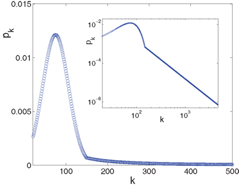
Figure 3. The in-degree distribution, p_k, plotted in both linear (main plot) and in log-log (inset) coordinates. Parameters used for the Gaussian are: k_cen = 75, σ = 31, k_min = 20 while the power law tail p ∼ B•k⁻² goes from k_tail = 150 to k_max = 4,680 and its pre-factor is B = 15.65. This normalizes the distribution to integral 1. The log-log scale in the inset highlights the power law tail, while the linear scale of the main plot accentuates the Gaussian that dominates the majority of the population.

Figure 4 shows our main result, in which an exponential growth rate is reproduced in a simulation employing the in-degree distribution of Figure 3. This exponential phase is followed by a super-exponential phase, in which the majority of the network ignites. The majority has in-degree defined by the Gaussian distribution and therefore they fire practically simultaneously. Since we tailored Φ(t), the growth during the exponential phase is indeed by a factor of 30, similar to the experimental one. However, the experimental graphs describe the momentary activity while Φ is the total fraction of active neurons and these do not turn off. The experiment is therefore probably better described by the derivative of Φ, shown in red. It can be clearly seen that in fact Φ and behave very similarly.

FIGURE 4

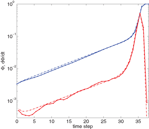
Figure 4. Growth rate of burst for tailored distribution from both numerical simulation using 500,000 neurons (solid lines) and iteration of Eq. 2 (dashed lines). Blue lines show overall firing fraction Φ for each time step. The red curves show the numerical derivative, The initial slowing down (the dip in the derivative) is due to a clearly evident “bottleneck” in the simulation, during which the firing almost ceases to propagate. The parameters used are f = 0.0033, α = 0.03, and k_min = round (m(1 + α)) = 16, k_max = round (m(1 + α)/f) = 4,680.

We can also compare the simulations of the network with the numerical solution of the model. For this we use the iterative scheme defined by Eq. 2 to propagate the activity of the network. This is shown (in dashed lines) in Figure 4. The excellent congruence of the simulation and the mean-field equation gives verification for the use of our mean-field model. The success relies on the absence of large deviations and insignificance of fluctuations, which is true in our model and experiment, due to the benign behavior of the degree distribution and the large number of participating neurons. The only deviation from this agreement is at the initial steps, where only a small number of leaders are firing.

In summary, from the quantitative comparison we find that the model has an exponential initial transient if the in-degree distribution is mostly Gaussian, with 10% of the neurons in the power law tail, and that the highest k can be in the thousands.

When comparing these results with the experiment, we should remember that only 60 electrodes are being monitored. The exponential behavior that is observed over a large dynamic range, can be resolved since multiple firings at the same electrode are observed with a resolution better than 1 ms. In the simulation, in contrast, this is modeled by going to high numbers of neurons, each of which can only fire once.

Excitation-Dependent Threshold

At the end of Section “First-to-Fire Neurons Lead Bursts and Have Large Input Degree” we noted that the sensitivity of neurons can be changed either by varying the number of their inputs, or by varying their threshold. Up to now, we have assumed that the firing threshold in the neural network m is a constant that does not change as the burst develops, and varied the degree distribution instead. In this section, we examine the impact of keeping the connectivity distribution static, while “loading” the recruitment dynamics onto m by making it a dynamical variable that depends on the history of neuronal activation. Since varying either parameter (m or p_k) will lead to the same results, in principle one could then have any distribution p_k of input degree, and compensate by varying m. One would then have to verify that the necessary variations in m are biologically reasonable and feasible. In the experiment this happens via the competing processes of adaptation and facilitation. Since adaptation would work opposite the trend observed in the experiment, we discuss only the possibility of facilitation.

Facilitation of activity can occur if neurons that are already excited several times are easier to excite at the next time. By synaptic facilitation we mean the property of a synapse increasing its transmission efficacy as a result of a series of high frequency spikes. We examine here some of these effects by introducing, for the sake of simplicity, a threshold which is a function of the average firing state, m(Φ).

Given the time series of the firing fraction Φ(t) and a presumed degree distribution p_k, one can invert Eq. 6 or Eq. 7 to obtain:

where K(P) is the inverse to the cumulative function (such an inverse function exists since P is monotonic).

It is particularly interesting to ask if the power law degree distribution p_k ∼ k⁻², supports a biologically feasible form of m(Φ), following the initial exponential regime where m should be constant. In this case the cumulative function is

where k_min and k_max are the limits of the distribution. The inverse function is

To further advance we need to model the burst itself, which grows exponentially at first, then grows even faster, at a super-exponential rate and finally saturates when all the network has fired. This behavior can be described by the function:

with a parameter to be determined from comparison to the experiment. This kind of burst function starts as an exponential Φ(t) ∼ e^αt and begins to diverge after time steps, but reaches Φ(t) = 1 slightly before fully diverging, at

For this profile Plugging into Eq. 17 yields,

We see that m(Φ) starts from m(f) ≃ k_min/(1 + α) and ends at Therefore, m decreases by a ratio of which for the experimental parameters is around 5, i.e., from m(f) ≃ 15 to m(1) ≃ 3, a biologically reasonable variation. The actual value of m that we use in the simulation is that of the nearest integer obtained by rounding Eq. 17. Figure 5 shows the behavior of the burst as a function of time for the power law distribution p_k ∼ k⁻² with variable m(Φ).

FIGURE 5

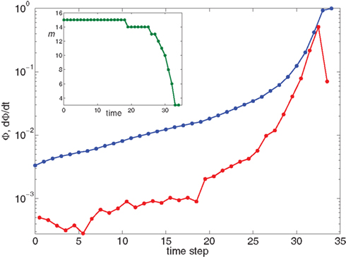
Figure 5. Growth rate of burst for k⁻² power law distribution and variable m(Φ(t)) using Eq. 17. The curve is calculated from numerical solution of the iteration Eq. 2. Blue line shows overall firing fraction Φ for each time step. The red curve shows the numerical derivative, The parameter used is time steps, and all other parameters are as in Figures 3 and 4. Inset: The threshold m(Φ(t)) decreases during the simulation as Φ increases according to Eq. 21. The value of m used in the simulation is the integer part of Eq. 21 hence the discrete jumps in its value. Until about t = 18 the value m is unchanged and the Φ(t) and profiles are exponential. Then m starts to decrease sharply and induces super-exponential growth of Φ(t).

Summary of Results

In summary, we have shown here that the experimental situation of an exponential transient followed by super-exponential growth can be well described in our model of an in-degree distribution that is k⁻² at high k but is Gaussian for the majority of the neurons. The initial transient of an exponential is determined directly by the power law tail of the degree distribution of Leaders.

The k-degree values needed to describe the data reach a maximum value that is many tens of standard deviations from the mean. Although the average value of the degree distribution remains in the region of 100, a few neurons (in a network of a million nodes) can have thousands of connections.

We remain with the question of how significant is the need for an exponent −2 in the power law distribution, and whether small deviations will change the exponential growth rate. Is there any logical or biological reason for this power law to be built up?

On the experimental side, the search for a few highly connected neurons would be needed. One possibility is that Leaders are neurons of a different species then that of the majority. Identifying them, investigating their properties and potentially intervening by disrupting their function are all important experimental goals.

Discussion

First-to-Fire Neurons and Leaders

In Eckmann et al. (2008) and Zbinden (2010, submitted) Leaders were defined through an intricate mathematical procedure. In particular, this definition allowed for exactly one Leader per burst, which ignites a pre-burst, and then a burst. In the present paper, a simpler definition is used, which amounts to taking into account basically all neurons which fire at the beginning of activity right after the initial fraction f. Since in the initial period of the burst there are only very few neurons active, the development of the burst depends critically on those neurons.

Within the Quorum Percolation model, high-k neurons activate the low k neurons. So the highest k neurons are the ones that trigger the burst. It follows that some of the highest k (in-degree) neurons are both first-to-fire and Leaders.

Looking only at in-degree is only part of picture. Indeed, high-k-classes are ignited first. However, their contribution to the firing propagation depends on the out-degree. Nodes with no outputs may fire early but contribute nothing to the ignition of others. Nevertheless, since we assumed that the in- and out-degree are uncorrelated, Leaders are among the early igniting nodes.

How Can we Get a Distribution of In-Degree Which is Gaussian with a k⁻² Tail?

An interesting question is what kind of growth and development process would lead to a distribution of in-degree that is essentially a Gaussian centered on a value of about k_cen = 75, but has a tail that goes like k_in ∼ k⁻², and can reach in-degree in the thousands, k_max ∼ 4,700.

We propose the following simplified and intuitive geometrical picture for how k_in and k_out are determined (see Figure 6). Each neuron in the culture has a spatial extent that is accessed by its dendrites (the “dendritic tree”) and characterized by a length scale ℓ (Figure 6A). The dendrites have no a priori preferred direction, and the dendritic tree is typically isotropic and characterized by a length scale r. Axons, on the other hand, go off in one direction, and their length determines the number of output connections the neuron will have. The dendritic tree is “presented” to axons of other neurons (Figure 6B). If the axon of a neuron happens to cross the dendritic tree of another neuron then, with some fixed probability (which we take for simplicity to be unity), a connection is made between the two neurons. The number of in-connections is therefore related to the size of the dendritic tree and to the number of axons crossing it, i.e., the density of axons. The number of out-connections of a neuron is determined by the length of its axon, the size of the dendritic tree of other neurons and the density of neurons.

FIGURE 6

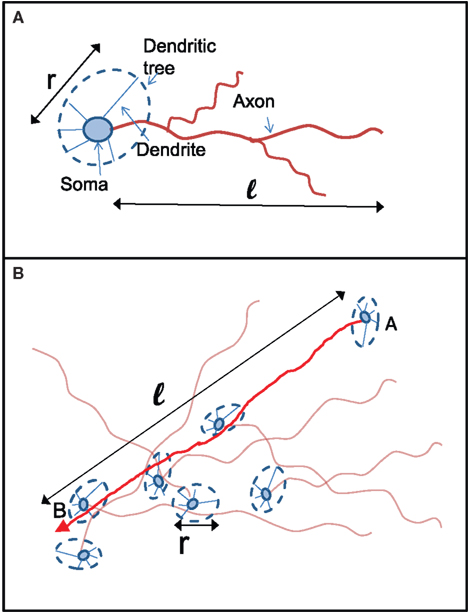
Figure 6. Schematic picture of the relation between axon and dendrite lengths ℓ and r to the number of connections k_in and k_out. (A) Two lengths characterize the connections of each neuron: its axonal length ℓ and the typical size of its dendritic tree r. While the dendritic tree is in general expected to be homogenous, it can have dendrites that go off much farther than the others. (B) A connection from Neuron A to Neuron B will be made if the trajectory of the axon extending from Neuron A will intersect the dendritic tree of Neuron B. The probability for that to happen depends on the probability P(ℓ) for A to have an axon of length longer than ℓ and on the probability p(r) for B to present a dendritic tree of cross section r.

There are two corresponding length distributions p(ℓ) and p(r) and a density n that determine the number of connections. p(ℓ) and p(r) are the probability distribution of the axon and dendrite lengths respectively, while n is the density of neurons per unit area.

The number of in-connections of a neuron is obtained by calculating the probability of an axon emitted from another neuron located a distance ℓ away to cross its dendritic tree (Figure 6B). To get the number of connections k_in for a neuron with dendritic tree of size r we look for the axons that will cross one of its dendrites:

Here is the cumulative sum of probability that the length of an axon exceeds ℓ (since it would then cross the dendritic tree). We ignore the slight r dependence of the lower limit of the integral. n is the density of neurons per unit area (about 500 neurons per mm²), and 2r/ℓ the angle extended by the dendritic tree as seen from the axon’s neuron of origin.

We now insert for p(ℓ) the Gaussian with power law tail:

if ℓ < ℓ_tail and p(ℓ) = B•ℓ−² for ℓ_tail < ℓ ≤ ℓ_max, with A ≫ B normalization factors.

For ℓ < ℓ_tail we get,

while for ℓ_tail < ℓ < ℓ_max:

The integral over P(ℓ) gives one constant term and one that goes as log(ℓ_max). Since the maximal length ℓ_max is determined by the size L of the culture dish, we remain with a term of log(L).

We get that the number of in-connections is

We are now in a position to ask where the tail of high connections arises. In principle, it could arise from fluctuations in the density n. The neural density is theoretically determined by throwing down a random set of points on the plane. In the experiment, the neuronal cultures do not exhibit clustering to such a degree that would induce so strong a fluctuation with such high density. To get the necessary range of a factor of 10 − 30 in k values that the theoretical explanation of the experimental data point to, we would need the density to change in a similar manner. This seems unrealistic. A further strong argument against fluctuations in density is that these would lead, in our picture, to a high number of input connections in one single neighborhood. In particular, this would lead to many more high-k neurons than the distribution allows for.

Thus we are led to the conclusion that the power law tail of k_in has its origin in the distribution of dendritic trees p(r). While the typical dendritic tree is probably a circle of with radius r = 100 − 200 μm, it may have outgrowths in one or more directions that reach as far as l = 1 − 2 mm but can, with small probability, go as far as the dish size L.

Trading off Static Connectivity Distribution for Dynamical Threshold

While the possibility of exchanging between elementary dynamics and connectivity statics does not come as a surprise, the lesson we take from the results of Section “Excitation-Dependent Threshold” is important indeed: One cannot distinguish, by observing network dynamics in and by itself, between a static connectivity-based mechanism and a mechanism that employs dynamics at the elementary level. While we tend to believe it is the connectivity that is dominant, one cannot rule out the neuron’s internal processes as a possible explanation for the dynamics.

When only a small fraction Φ of the network is active, the chances that a given neuron is activated at a high frequency are low. Hence, chances of changes in threshold as a result of synaptic or membrane dynamics are low. However, as the active fraction Φ of the network grows, the chances of a neuron to be bombarded at high frequency become higher; we could then get a dependence m(Φ), since changes in threshold (i.e., membrane dynamics) or synaptic efficacy (e.g., facilitation) are expected.

In many studies of biological networks, this ambiguity is somewhat neglected in favor of a more static view, largely due to lack of access to elementary level dynamics. In the case of neuronal excitability, single element dynamics is experimentally accessible, and the existence of dynamical-thresholds are well documented. Our results in Section “Excitation-Dependent Threshold” indicate that this is a sufficient explanation to the phenomenon of an early exponential recruitment rate followed by faster growth process.

The Effect of Limiting Size: One-Dimensional Cultures

Initiation of activity in 1D cultures seems to be very different from the Leaders scenario. In 1D cultures, we (Feinerman et al., 2007) have shown that the activity originates locally, at well defined “Burst Initiation Zones” (BIZs) that have a limited spatial extent. There are usually a small number of such BIZs, typically 1 or 2 per centimeter, that operate independently of each other. The BIZs are characterized by a high density of excitatory neurons and a low density of inhibitory ones. Firing activity that originates in a BIZ will propagate out as a wave-like front with a constant velocity, and invade the rest of the culture until all neurons have fired.

One explanation for the difference in behavior of BIZ and Leaders is in the dimensionality. However, the basic argument we presented for the number of input connections relates it to the multiplication of the area of the dendritic tree by the density of the axons that cross through this area. Since both the radius of the dendritic tree and the width of the line are on the order of 100 μm, there should be no difference in the first factor. As for the density of axons, there is no direct information, but also no compelling argument why 1D cultures should differ in this from 2D cultures.

A different possibility, and the one we believe to be correct, is just that there are too few neurons in the culture (Tlusty and Eckmann, 2009). That would impact on any small culture, both 2D and 1D. Changing the number of neurons has the largest effect on the realization of the tail of the probability distribution p_k, since high-k values have a low probability and will not be obtained. This can completely disrupt the form of the degree distribution. In turn, it also affects the value of the fraction of initial firing needed for ignition of the full culture.

The results of simulating excitation in varying numbers of neurons are given in Table 1.

TABLE 1

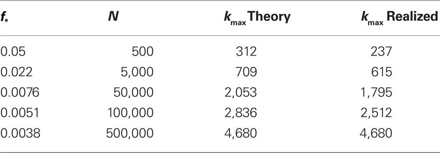
Table 1. Study of finite size networks: for small N networks, needs to be larger and the experimentally accessible k_max does not reach the theoretical prediction. This shows that the ignition process is less efficient for small N.

We immediately see that indeed depends strongly on N. A power law fit indicates that At about N = 200,000 the curve flattens out, and reaches the theoretical (N = ∞) value. The reason for this originates in the constraints imposed between and k_max, In any realization of finite size N, any k with p_k < 1/N is very unlikely to be observed. Since p_k ∼ k⁻² both k_max and are constrained by the N^−1/2. We can conclude that within the Quorum Percolation model smaller cultures require a much larger fraction of initial activity to sustain a burst.

Acknowledgments

We are indebted to Shimon Marom for many stimulating discussions and in particular for suggesting the equivalent effect of in-degree distributions and neuronal thresholds. We also thank Shimshon Jacobi, Maria Rodriguez Martinez and Jordi Soriano. This research was partially supported by the Fonds National Suisse, the Israel Science Foundation grants number 1320/09 and 1329/08, Minerva Foundation Munich Germany and the Einstein Minerva Center for Theoretical Physics. Olav Stetter acknowledges support from the German Ministry for Education and Science (BMBF) via the Bernstein Center for Computational Neuroscience (BCCN) Göttingen (Grant No. 01GQ0430).

Conflict of Interest Statement

The authors declare that the research was conducted in the absence of any commercial or financial relationships that could be construed as a potential conflict of interest.

References

Alvarez-Lacalle, E., and Moses, E. (2009). Slow and fast pulses in 1-d cultures of excitatory neurons. J. Comput. Neurosci. 26, 475–493.

Pubmed Abstract | Pubmed Full Text | CrossRef Full Text

Amit, D. J., Gutfreund, H., and Sompolinsky, H. (1985). Spin-glass models of neural networks. Phys. Rev. A 32, 1007–1018.

Pubmed Abstract | Pubmed Full Text | CrossRef Full Text

Bollobas, B. (1998). Modern Graph Theory. New York: Springer.

Breskin, I., Soriano, J., Moses, E., and Tlusty, T. (2006). Percolation in living neural networks. Phys. Rev. Lett. 97, 188102.

Pubmed Abstract | Pubmed Full Text | CrossRef Full Text

Cohen, O., Keselman, A., Moses, E., Rodriguez-Martinez, M., Soriano, J., and Tlusty, T. (2010). Quorum percolation in living neural networks. Europhys. Lett. 89, 18008.

CrossRef Full Text

Eckmann, J.-P., Jacobi, S., Marom, S., Moses, E., and Zbinden, C. (2008). Leader neurons in population bursts of 2d living neural networks. New J. Phys. 10, 015011.

CrossRef Full Text

Eytan, D., and Marom, S. (2006). Dynamics and effective topology underlying synchronization in networks of cortical neurons. J. Neurosci. 26, 8465–8476.

Pubmed Abstract | Pubmed Full Text | CrossRef Full Text

Feinerman, O., Segal, M., and Moses, E. (2005). Signal propagation along unidimensional neuronal networks. J. Neurophysiol. 94, 3406–3416.

Pubmed Abstract | Pubmed Full Text | CrossRef Full Text

Feinerman, O., Segal, M., and Moses, E. (2007). Identification and dynamics of spontaneous burst initiation zones in unidimensional neuronal cultures. J. Neurophysiol. 97, 2937–2948.

Pubmed Abstract | Pubmed Full Text | CrossRef Full Text

Golomb, D., and Ermentrout, G. B. (1999). Continuous and lurching traveling pulses in neuronal networks with delay and spatially decaying connectivity. Proc. Natl. Acad. Sci. U.S.A. 96, 13480–13485.

Pubmed Abstract | Pubmed Full Text | CrossRef Full Text

Golomb, D., and Ermentrout, G. B. (2002). Slow excitation supports propagation of slow pulses in networks of excitatory and inhibitory populations. Phys. Rev. E 65, 061911.

CrossRef Full Text

Jacobi, S., and Moses, E. (2007). Variability and corresponding amplitude–velocity relation of activity propagating in one-dimensional neural cultures. J. Neurophysiol. 97, 3597–3606.

Pubmed Abstract | Pubmed Full Text | CrossRef Full Text

Maeda, E., Robinson, H. P., and Kawana, A. (1995). The mechanisms of generation and propagation of synchronized bursting in developing networks of cortical neurons. J. Neurosci. 15, 6834–6845.

Pubmed Abstract | Pubmed Full Text

Osan, R., and Ermentrout, B. G. (2002). The evolution of synaptically generated waves in one- and two-dimensional domains. Physica D 163, 217–235.

CrossRef Full Text

Provost, J. P., and Vallee, G. (1983). Ergodicity of the coupling constants and the symmetric n-replicas trick for a class of mean-field spin-glass models. Phys. Rev. Lett. 50, 598–600.

CrossRef Full Text

Soriano, J., Rodriguez-Martinez, M., Tlusty, T., and Moses, E. (2008). Development of input connections in neural cultures. Proc. Natl. Acad. Sci. U.S.A. 105, 13758–13763.

Pubmed Abstract | Pubmed Full Text | CrossRef Full Text

Streit, J., Tscherter, A., Heuschkel, M. O., and Renaud, P. (2001). The generation of rhythmic activity in dissociated cultures of rat spinal cord. Eur. J. Neurosci. 14, 191.

Pubmed Abstract | Pubmed Full Text | CrossRef Full Text

Tlusty, T., and Eckmann, J.-P. (2009). Remarks on bootstrap percolation in metric networks. J. Phys. A 42, 205004.

CrossRef Full Text

van Hemmen, J. L. (1982). Classical spin-glass model. Phys. Rev. Lett. 49, 409–412.

CrossRef Full Text

Zbinden, C. (2010). Leader Neurons in Living Neural Networks and in Leaky Integrate and Fire Neuron Models. PhD thesis, University of Geneva, Geneva. Available at http://archive-ouverte.unige.ch/unige:5451.