1
Department of Human and Computer Intelligence, Ritsumeikan University, Shiga, Japan
2
Laboratory for Neural Circuit Theory, RIKEN Brain Science Institute, Saitama, Japan
3
Department of Physics, Graduate School of Science, Kyoto University, Kyoto, Japan
Information is transmitted in the brain through various kinds of neurons that respond differently to the same signal. Full characteristics including cognitive functions of the brain should ultimately be comprehended by building simulators capable of precisely mirroring spike responses of a variety of neurons. Neuronal modeling that had remained on a qualitative level has recently advanced to a quantitative level, but is still incapable of accurately predicting biological data and requires high computational cost. In this study, we devised a simple, fast computational model that can be tailored to any cortical neuron not only for reproducing but also for predicting a variety of spike responses to greatly fluctuating currents. The key features of this model are a multi-timescale adaptive threshold predictor and a nonresetting leaky integrator. This model is capable of reproducing a rich variety of neuronal spike responses, including regular spiking, intrinsic bursting, fast spiking, and chattering, by adjusting only three adaptive threshold parameters. This model can express a continuous variety of the firing characteristics in a three-dimensional parameter space rather than just those identified in the conventional discrete categorization. Both high flexibility and low computational cost would help to model the real brain function faithfully and examine how network properties may be influenced by the distributed characteristics of component neurons.
Identical fluctuating currents elicit similar spike trains from the same neuron (Bryant and Segundo, 1976
; Mainen and Sejnowski, 1995
), but there are significant differences in the spike trains of different neurons to the same currents. The brain comprises a variety of neurons possessing such different response characteristics (Shinomoto et al., 2009
). A model that is capable of precisely reproducing spike response of any neuron to any input current is an essential first step to both building a brain simulator (Brette et al., 2007
; Diesmann et al., 1999
; Gewaltig and Diesmann, 2007
; Izhikevich and Edelman, 2008
; Markram, 2006
; McIntyre et al., 2004
; Plesser and Diesmann, 2009
), and understanding the computational mechanisms of neurons (Abeles, 1991
; Beggs and Plenz, 2003
; Diesmann et al., 1999
; Ikegaya et al., 2004
).
The Hodgkin–Huxley (HH) model is a standard model for describing neuronal firing, and has been continually revised by including ionic channels to reproduce standard electrophysiological measurements of cortical neurons (Hodgkin and Huxley, 1952
; Koch, 1999
). It has recently become possible to use elaborate simulation platforms, such as NEURON (Hines and Carnevale, 1997
) and GENESIS (Bower and Beeman, 1995
), for reproducing experimental data. Because of nonlinearity and complexity, however, parameter optimization of the HH type models is a notoriously difficult problem (Achard and De Schutter, 2006
; Goldman et al., 2001
; Huys et al., 2006
), and these models require a high computational cost, which hinders performing the simulation of a massively interconnected network.
For these reasons, simplified phenomenological models such as the leaky integrate-and-fire (LIF) model (Stein, 1965
) have been proposed, and these models have been useful for studying learning, memory, and the dynamics of neural networks (Gerstner and Kistler, 2002
; Hansel and Sompolinsky, 1998
). Due to this simplification, many details of the biophysical properties of neurons are abandoned. However, simplified models that extend beyond the qualitative description of neuronal firing have been developed (Fourcaud-Trocmé et al., 2003
; Gerstner and Kistler, 2002
; Izhikevich, 2004
). Nonlinear integrate-and-fire models have been successfully applied to some typical neurons (Badel et al., 2008
; Brette and Gerstner, 2005
). The spike response model (SRM) exhibits fairly good predictive performances (Jolivet et al., 2004
, 2006
; Kobayashi and Shinomoto, 2007
). It is feasible to fit the LIF model to neurophysiological data, in particular, to reproduce the statistical features in interspike intervals (Inoue et al., 1995
; Lansky and Ditlevsen, 2008
; Lansky et al., 2006
; Tuckwell and Richter, 1978
), but parameter optimization in the SRM or nonlinear models for predicting spike times is a difficult problem because of their nonlinearity or a large number of parameters.
In this study, we propose a minimal model for accurately predicting a rich variety of spike responses in vitro and develop a procedure for optimizing model parameters. The model consists of the simple leaky integrator and a multiple-timescale adaptive threshold, which is referred to as the MAT model. The MAT model has low computational cost and high predictive performances for both stationary and nonstationary fluctuating currents. The model is adaptable to various types of neurons, including regular spiking (RS), intrinsic bursting (IB), and fast spiking (FS) neurons, by simply fitting three parameters, and is also capable of describing the spike patterns of chattering (CH) neurons.
Multi-Timescale Adaptive Threshold Model
The dynamics of a nonresetting leaky integrator proposed in this study is given as,

where τm, V(t), R, and I(t) are the membrane time constant, model potential, membrane resistance, and input current, respectively. When the model potential reaches the spike threshold θ(t), a spike is generated. In our model, V(t) is not reset even if the model assumes spikes. Instead, the spike threshold increases when the model assumes a spike and then decays toward the resting value. In the standard adapting threshold model, the spike threshold θ(t) decays exponentially (Brandman and Nelson, 2002
; Chacron et al., 2003
; Geisler and Goldberg, 1966
). In the present study, we extended this adaptive threshold rule into a MAT rule.
where tk is the kth spike time, L is the number of threshold time constants, τj (j = 1,…,L) are the jth time constants, αj (j = 1,…,L) are the weights of the jth time constants, and ω is the resting value. To avoid singular bursting, we introduced an absolute refractory period of 2 ms during which the model is not allowed to fire even if the membrane potential exceeds the threshold. If the membrane potential still remains above threshold for the 2 ms, the model assumes another spike. We refer to the model as the MAT(L) model, including a single timescale model as the MAT(1). Here, we integrate the equation with the Euler method at a step size of 0.001 ms and verify results with backward Euler.
Fitting Procedure
The MAT(L) model is specified by the 2L + 3 parameters {τm, R, τj, αj (j = 1, 2,…,L), ω}. The model comprises two dynamic components: the membrane potential and spike threshold (Figure 1
A). We first determined the parameters of the membrane potential dynamics {τm, R} by fitting the voltage response to fluctuating currents with a nonresetting leaky integrator. These parameters were optimized for minimizing the squared error,
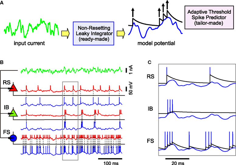
Figure 1. A variety of firing patterns represented by the MAT* model. (A) Schematic representation of the MAT model: A ready-made nonresetting leaky integrator estimates the intrinsic subthreshold membrane potential. If the estimated potential (blue trace) hits a threshold (black trace) from below, the model assumes a spike and lifts the threshold. The adaptive threshold spike predictor can be tailored to individual neurons by adjusting the amount of fast (10 ms) and slow (200 ms) dynamics. (B) Voltage responses of the three types of neurons, regular spiking (RS), intrinsic bursting (IB), and fast spiking (FS) (red traces) induced by the same fluctuating currents (the green trace at the top): The estimated potentials and predicted spikes with the MAT* model (blue traces) are depicted below the real membrane potentials.The model potentials computed for the same current are identical among neurons. Predicted spikes are connected by dotted lines to the real spikes if they coincided within 2 ms. Model parameters: RS: α1 = 37 mV, α2 = 2.0 mV, ω = 19 mV, IB: α1 = 1.7 mV, α2 = 2.0 mV, ω = 26 mV, FS: α1 = 10 mV, α2 = 0.002 mV, ω = 11 mV; common parameters for the three neurons: τm = 5 ms, R = 50 MΩ; L = 2, τ1 = 10 ms, τ2 = 200 ms. (C) Magnified view of the boxed area in (B): Different dynamics are manifested for the identical model potentials due to the difference in the three parameters of MAT* threshold dynamics.
We determined the membrane time constant τm for 34 neurons (see Section “Electrophysiological Recordings”). The membrane time constant ranged from 2.0 to 12.0 ms, with a mean ± SD of 6.2 ± 2.2 ms. By confirming that predictive performance is not sensitive to this parameter, we adopted a common membrane time constant for all neurons, τm = 5 ms. The resistance R simply scales the potential and is unrelated to the spike time prediction of the model; therefore, we adopted a common resistance R = 50 MΩ for all neurons.
Second, we determined the parameters for the spike threshold dynamics {τj, αj, ω}. In this study, we examined three cases, single timescale (L = 1), two timescales (L = 2), and three timescales (L = 3). We selected a set of time constants τj from trial parameters (10, 50, and 200 ms), so that the model performance defined below is maximized on average for all neurons. Given a set of time constants, the firing properties of individual neurons are solely represented by {αj, ω}. These tailor-made parameters were optimized so that the coincidence factor Γ defined below was maximized for the set of sample data comprising three input currents (mean ± SD, 0.42 ± 0.14, 0.37 ± 0.25, and 0.29 ± 0.19 nA) and the corresponding spike trains. We used the Nelder–Mead method (Nelder and Mead, 1965
) for the maximization procedure.
Assessment of Predictive Performance
The performance of the spike time prediction is assessed with a coefficient measuring the degree of coincidence of a model spike train with a real spike train. Among various methods for measuring the similarity between two spike trains (Tsubo et al., 2004
; Victor and Purpura, 1996
), we adopted here the coincidence factor Γ (Jolivet et al., 2004
, 2006
, 2008a
; Kobayashi and Shinomoto, 2007
), defined by
where Ndata and Nmodel, respectively, represent the numbers of spikes in the data and the model, Ncoinc is the number of coincident spikes with an allowable range of time Δ. Here, Ncoinc is subtracted by the expected number of coincidences between the data and the random Poisson spikes of the given rate, 〈Ncoinc〉 = 2vNdata, so that the coefficient takes a value close to 0 for mutually independent spike trains. The coefficient is divided by 1 − 2vΔ so that it takes a value 1 if all the spikes coincided within Δ. In this study, Δ is chosen as 2 ms.
Each neuron model was tailored to every neuron using sample current–voltage data, by maximizing the coincidence score Γ. The model was then tested with a new current to see how well it predicted spike times. The predictive performances was assessed based on the coincidence scores normalized with the trial-to-trial variation of the experiments, defined by
Various models were compared based on the predictive scores ΓA evaluated for individual neurons under conditions in which the neurons were firing at rates close to 10 and 30 Hz (in case of FS, 70 and 140 Hz) respectively, with different degrees of fluctuation (SD/mean, 0.35 and 0.70). We took into account the predictive scores ΓA, provided that spikes were elicited within a range from 5 to 200 Hz, and with a degree of trial-to-trial reproducibility, Γexperiment-experiment > 0.1. As a result, 119 data among 4 × 34 = 136 data were available, and each neuron was evaluated by the average score for the three or four data.
Electrophysiological Recordings
The current injection experiments for 34 neurons in layers 2/3 and 5 of the rat motor cortex were performed exclusively for the present study, whereas the conductance injection experiments for nine neurons were performed previously for the study of Miura et al. (2007)
. We abbreviate the animal preparation details that are common with the methods published in the paper, and describe the essentials needed in the present study. All experiments were performed in accordance with animal protocols approved by the Experimental Animal Committee of the RIKEN Institute.
Wistar rats (postnatal days, 17–27) were deeply anesthetized with diethyl ether gas and then decapitated. Data used for examining the spike time prediction was taken from rat cortical slices (400-μm thick) sectioned using a microslicer (PRO-7; Dosaka, Kyoto, Japan). After incubation for 30 min at 31 °C and at least 1 h of recovery at room temperature, each slice was transferred to a submerged-type recording chamber continuously circulating with normal artificial cerebrospinal fluid (ACSF; 32°C), which consisted of (in mM) 124 NaCl, 2.5 KCl, 1.2 KH2PO4, 26 NaHCO3, 1.2 MgSO4, 2.5 CaCl2, and 25 D-glucose and was saturated with 95% O2 and 5% CO2 gas. We recorded in the current-clamp or conductance-clamp whole-cell configuration from the soma using patch pipettes filled with (in mM) 140 K-gluconate, 2 NaCl, 1 MgCl2, 10 HEPES, 0.2 EGTA, 2 5-ATPNa2, 0.5 GTPNa2, and 10 biocytin, pH 7.4 (Tsubo et al., 2007
). The neuron membrane potentials were recorded using a current clamp amplifier (Axoclamp 2B; Molecular Devices, Union City, CA, USA) in the conventional bridge mode. Recorded signals were digitized using an analog–digital interface (Digidata 1322A; Molecular Devices) at 40 kHz in current injection experiments and 50 kHz in conductance injection experiments. To block the spontaneous input via AMPA, NMDA, and GABAA receptors, a cocktail of 6-cyano-7-nitroquinoxaline-2,3-dione (10 μM; Sigma, St Louis, MO, USA), DL-2-amino-5-phosphonopentanoic acid (25 μM; Sigma), and bicuculline methiodide (30 μM; Sigma) was added to ACSF and bath-applied to the cortical slices. Based on the criteria suggested by Nowak et al. (2003)
, the 34 recorded cells were classified into 22 RS, 8 IB, and 4 FS neurons.
For the current injection experiments, the input current
was prepared by mimicking natural inputs comprising the synaptic input from thousands of unitary excitatory and inhibitory post-synaptic currents (EPSCs and IPSCs) with amplitudes Iexc = 0.1 nA and Iinh = 0.033 nA, and decay-time constants τexc = 1 ms and τinh = 3 ms, respectively (Tsubo et al., 2004
). A = 0.1–1.2 is a scale factor, and the voltage dependence of EPSCs and IPSCs were neglected (Stevens and Zador, 1998
). Arrival time of excitatory and inhibitory spikes {tk} and {tj} were drawn from the Poisson processes with statistical rates rexc and rinh, respectively. During the stationary fluctuating current trials, the statistical rates were fixed so that the mean ± SD of the input currents were 0.40 ± 0.14 nA (rexc = 6.88 kHz, rinh = 2.88 kHz) or 0.40 ± 0.28 nA (rexc = 24.52 kHz, rinh = 20.52 kHz). Then, these injected currents were scaled by a factor A; for instance, the current ID “0.20 ± 0.14 nA” indicates the current made from “0.40 ± 0.28 nA” scaled by 0.5. For nonstationary current trials, the statistical rates were sinusoidally time-varied so that the mean ± SD of the input currents were [0.30 + 0.10sin (2πt)] ± [0.21 + 0.07sin (2πt/2)] nA. One trial lasted 5 s and the identical currents were repeated twice with a 15-s intertrial interval.
For conductance injection experiments, the excitatory and inhibitory input conductances gexc(t) and ginh(t) were described by the Ornstein–Uhlenbeck processes (OUP; Uhlenbeck and Ornstein, 1930
) with time constants τexc = 2.7 ms and τinh = 10.5 ms, mean conductances gexc0 and ginh0 = Bgexc0, and SDs σexc = gexc0/2 and σinh = Bgexc0/4, respectively. The excitatory mean conductance gexc0 was set to 0.018 and 0.024 μS for parameter determination, and 0.012 and 0.030 μS for model assessment. The ratio of excitatory and inhibitory mean conductance B = gexc0/ginh0 was set to −0.348 and −0.370, respectively. Using a conductance clamp method (Robinson and Kawai, 1993
; Sharp et al., 1993
), we injected these conductances as a fluctuating current I(t):

where V(t) is the recorded membrane potential, and Eexc = 0 mV and Einh = −75 mV are the reversal potential of excitatory and inhibitory synaptic currents, respectively. One trial lasted 10 s. In each trial, a set of time constants, mean values, and SDs of excitatory and inhibitory OUP conductances were fixed. The identical conductances were repeated twice with a 30-s intertrial interval.
We first study the timescales essential for predicting spike times of cortical neuron in vitro. We design the minimal MAT model for predicting spike times. Second, we show that the MAT model accurately predicts the spike responses of a variety of cortical neurons and those for various input conditions by adjusting only three parameters. We compare the predictive performances of this model with three standard models: a HH model, LIF model, and SRM. The parameters of each model are fitted to data, using widely accepted methods (Appendix).
Timescales Essential for Predicting Spikes
To study the timescales essential for predicting spike times, we compare the predictive performances of MAT(L) models. We examine three cases, single timescale (L = 1), two timescales (L = 2), and three timescales (L = 3). Timescales of the adaptive threshold dynamics τj are selected from 10, 50, and 200 ms. The predictive performances achieved by all possible combinations of the three timescales are summarized in Table 1
. The optimal timescale for the MAT(1) model is τ1 = 50 ms. The optimal timescales for the MAT(2) model are τ1 = 10 ms and τ2 = 200 ms, and this model resulted in the best performance for all combinations of the three timescales. It is noteworthy that the predictive performance of this MAT(2) model was even better than that of the MAT(3) model. Though adding parameters may improve fitting, a wider class model does not necessarily acquire the better predictive ability by the learning from a finite set of samples, because a model with overabundant parameters may exhibit overfitting for finite samples. We refer to the MAT(2) model with τ1 = 10 ms and τ2 = 200 ms as the MAT* model. In the following subsections, we adopt the MAT* model for predicting spike times.
Free Parameters of the MAT* Model Representing Different Kinds of Neurons
Identical fluctuating currents induce different responses in different neurons (Figure 1
B). Neurons are categorized into three types based on conventional categorical criteria given by McCormick et al. (1985) and Nowak et al. (2003)
: RS, IB, and FS. A variety of spiking patterns among these neurons elicited by the same input current are predicted simply by selecting three parameters of the MAT* model. It should be noted that the model potentials are computed with the same leaky integrator and therefore are identical for all neurons. In the MAT* model, different firing patterns are manifested solely due to the difference in the threshold dynamics (Figure 1
C).
For a set of 34 neurons, three parameters α1, α2, and ω of the MAT* model are determined so that the fraction of common spikes between the model and experiment is maximized for the sample dataset. RS, IB, and FS neurons that are categorized based on the conventional categorical criteria are separately localized in a component plane of the fast and slow threshold dynamics α1 and α2 (Figure 2
A).
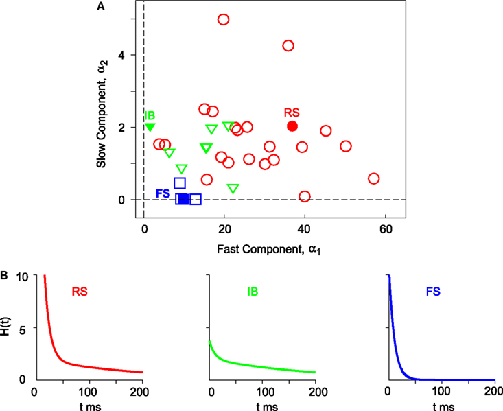
Figure 2. Components of the fast and slow threshold dynamics of the MAT* model. (A) The coefficients are determined for 34 neurons with respect to the sample data comprising three input currents and the induced spikes. The 22 regular spiking (RS), 8 intrinsic bursting (IB), and 4 fast spiking (FS) neurons are depicted with circles, triangles, and squares, respectively. (B) Double exponential functions H(t) (Eq. 3) of the three types of neurons (three closed marks). Model parameters are the same as in Figure 1
.
H(t) (Eq. 3) are depicted with respect to three prototypical neurons (Figure 2
B): RS neurons contain both large amounts of fast α1 and slow α2 components of the threshold dynamics, whereas IB neurons contain a small amount of the fast component α1 and a large amount of the slow component α2, and FS neurons contain a small amount of the fast component α1 and a negligible amount of the slow component α2.
Model Performance
We compare the MAT* model with a HH model, LIF model, and SRM for their ability to predict spike times elicited from fluctuating currents by neurons in a rat cortical slice preparation (Figure 3
B). In each model, the model parameters are optimized from sample data consisting of injected currents and the induced membrane potential of an individual neuron, and then test with a new current for the ability to predict spike times of the same neuron. The predictive ability is evaluated with a coincidence factor Γ between predicted spikes and target spikes within a range of 2 ms (see Section “Materials and Methods”). Identical fluctuating currents elicit similar spike trains from the same neuron (Figure 3
A). The score is normalized by variation among experimental trials so that the best prediction could be evaluated as ΓA close to 1. The mean ± SD of the predictive scores ΓA are evaluated for 34 neurons (Figure 3
C).
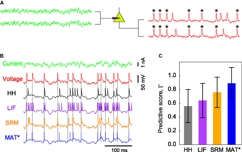
Figure 3. Spike times predicted by the four models. (A) Schematic figure of the current injection experiment: Nearly identical spike sequences are elicited from identical fluctuating currents for each neuron. Asterisks mark the spikes that coincide within 2 ms in two experimental trials. (B) Voltage response of a given neuron to a novel input current, and the spike times predicted with the HH, LIF, SRM, and MAT* models: Dotted lines represent the experimental spike times. Model parameters: HH: C = 86 pF, gNa = 750 nS, gKd = 210 nS, gM = 210 nS, gL = 0.6 nS, VT = −61 mV; LIF: θ = 25 mV; SRM: α = 12 mV, ω = 13 mV, τα = 50 ms; MAT*: α1 = 37 mV, α2 = 2 mV, ω = 19 mV. (C) Predictive scores ΓA evaluated for the four models: The error bars indicate SDs among all neurons examined.
The HH model is fitted to experimental conductance data, but is weak in its ability to predict spike times, resulting in a predictive scores ΓA = 0.51 ± 0.26. The LIF model and SRM with an adaptive threshold yield ΓA = 0.66 ± 0.26, and ΓA = 0.70 ± 0.26, respectively. The MAT* model achieves the best predictive score of ΓA = 0.89 ± 0.21.
Prediction of Spike Responses to Nonstationary Current Inputs
In addition to the stationary situations in which synaptic input currents fluctuate finely, we also mimic the nonstationary situation in which behavioral stimuli or motor commands greatly modulate the input currents. In this study, the temporal mean of the fluctuating current is modulated sinusoidally with a period of 1 s, while the SD of fluctuation is slowly modulated with a period of 2 s (Figure 4
A). The predictive scores ΓA evaluated for an RS neuron for the entire 5 s interval are 0.49, 0.78, 0.64, and 0.84 for the HH, LIF, SRM, and MAT* models, respectively.
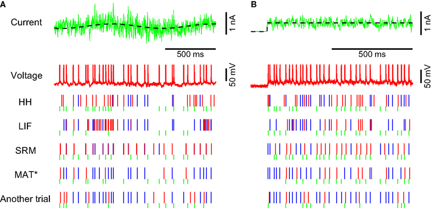
Figure 4. Spike times for nonstationary input currents. Voltage responses of two RS neurons (red traces) induced by a nonstationary fluctuating current (the green trace at the top). The mean of the current is depicted with a black dotted line. The spike times predicted by the HH, LIF, SRM, and MAT* models are depicted below. The model spikes that hit the experimentally obtained spikes are indicated by the blue bars, the excess spikes are indicated by the red bars, and the passes are indicated by the green short bars. The lowest column represents another experimental trial with identical fluctuating current. (A) The mean of the current is modulated sinusoidally with a period of 1 s, while the SD of the current is modulated with a period of 2 s. The predictive scores ΓA of the models fitted to the entire 5 s interval are 0.49, 0.78, 0.64, and 0.84 for the HH, LIF, SRM, and MAT* models, respectively. Parameters: HH: C = 70 pF, gNa = 960 nS, gKd = 25 nS, gM = 4 nS, gL = 5 nS, VT = −38 mV; LIF: θ = 22 mV; SRM: α = 15 mV, ω = 20 mV, τα = 50 ms; MAT*: α1 = 56 mV, α2 = 5 mV, ω = 9 mV. (B) At the onset of a current with a mean ± SD of 0.39 ± 0.13 nA, the predictive scores ΓA evaluated for the initial 1 s interval are 0.49, 0.52, 0.38, and 0.68. Parameters: HH: C = 83 pF, gNa = 840 nS, gKd = 250 nS, gM = 130 nS, gL = 0 nS, VT = −63 mV; LIF: θ = 21 mV; SRM: α = 11 mV, ω = 5.5 mV, τα = 50 ms; and MAT*: α1 = 23 mV, α2 = 1.9 mV, ω = 11 mV.
The four models are also compared for their ability to predict transient firing rate adaptation of an RS neuron to the initiation of current injections. All preexisting models fail to reproduce the transient adaptation, but the MAT* model is able to predict the adaptive phenomena (Figure 4
B). The predictive scores ΓA evaluated for the initial 1 s interval are 0.49, 0.52, 0.38, and 0.68 for the four models.
In this way, the MAT* model is superior to the three standard models in predicting spikes for stationary fluctuating currents, slowly modulated nonstationary currents, and the onset of current injection.
Prediction of Spike Responses to Conductance Inputs
In addition to the current injection experiments, we also examine the predictive ability of the four models for the conductance injection experimental data. We analyze the data assuming that τm = 5 ms and R = 50 MΩ. Predictive scores ΓA for the HH, LIF, SRM, and MAT* models are 0.52 ± 0.23, 0.64 ± 0.17, 0.45 ± 0.21, and 0.84 ± 0.18; thus, the MAT* model consistently exhibits a better performance for predicting spike times.
A Variety of Responses of MAT* Model to a Rectangular Current
We also explore a space of the parameters α1, α2, and ω to examine if MAT* model can produce the typical firing responses to a rectangular current. As we confirmed in the application to biological data, the MAT* model can represent response characteristics of the RS, IB, and FS neurons. Numerical simulations were performed with various parameter values (Figures 5
A,B).
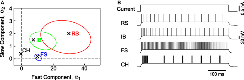
Figure 5. Components of fast and slow dynamics and the model simulations. (A) Distributions of MAT* parameters α1 and α2 for RS, IB, and FS neurons are represented as the 1/2 quantiles of the Gaussian distributions fitted to the data in Figure 3
. (B) Spikes generated by a rectangular current of 0.60 nA (500 ms): The parameters of the MAT* model are, RS: α1 = 30 mV, α2 = 2.0 mV, ω = 20 mV, IB: α1 = 7.5 mV, α2 = 1.5 mV, ω = 19 mV, and FS: α1 = 10 mV, α2 = 0.2 mV, ω = 10 mV. It is possible to mimic the chattering phenomenon by choosing a negative value for the fast component, CH: α1 = −0.5 mV, α2 = 0.4 mV, ω = 26 mV.
It is noteworthy that the specific firing pattern of the “chattering” (CH) neuron (Gray and McCormick, 1996
) can be reproduced in the parameter range α1 < 0 and α2 > 0: A negative factor for the fast timescale, α1 < 0, lowers the firing threshold and initiates bursting with the given absolute refractory period. However, as bursting continues, the positive factor for the longer timescale, α2 > 0, accumulates and eventually terminates bursting. This cycle is repeated to produce “chattering”.
We have proposed a new model named “MAT” that is equipped with a multi-timescale adaptive threshold predictor and a nonresetting leaky integrator. The minimal MAT* model is capable of reproducing a rich variety of neuronal spike responses from RS, IB, and FS neurons by simply adjusting three adaptive threshold parameters (Figure 1
). The model expresses a variety of the firing characteristics rather than a conventional discrete categorization (Figure 2
). The MAT* model provides the highest predictive performance among four models including the conventional HH, LIF, and SRM (Figure 3
), and is superior for predicting spikes for greatly fluctuating inputs (Figure 4
). It also has a potential for generating the specific firing pattern of the CH neurons (Figure 5
).
Biological Entities Related to Adaptive Threshold Dynamics
An essential component of the MAT* model is the introduction of multiple time constants into the threshold dynamics. Adaptive threshold time constants were selected from among trial parameters of 10, 50, and 200 ms. These time constants would be related to biological ionic currents (Hille, 2001
; Koch, 1999
): [10 ms]: Fast transient Na+ current and delayed rectifier K+ current, [50 ms]: hyperpolarization-activated cation current, and K+ A-current, and [200 ms]: noninactivating K+ current, hyperpolarization-activated cation current, and Ca+2-dependent K+ current.
Eventually, 10 and 200 ms were selected for the MAT* model based on its predictive performance. Different types of neuronal firing can be reproduced and predicted by simply adapting components of shorter and longer timescale dynamics to experimental data. RS, IB, and FS neurons are separately localized in a component plane of the two timescale dynamics. RS neurons have a large amount of both shorter and longer timescale threshold dynamics; IB neurons have a smaller amount of shorter one; and FS neurons have a small amount of shorter one and a negligible amount of longer one. If the firing characteristics are modified by some external operations on ion channel densities, it would be worthwhile to fit the MAT model and examine how the weight parameters vary in such a process.
The effectiveness of our MAT model implies that neuronal firing dynamics are mainly governed by multiple refractory effects with different timescales, and the characteristics are mainly determined by their combination. The time constants (10, 50, and 200 ms) were chosen as trial parameters, and turned out to be good. When targeting individual neurons, there is still room for improvement in performance, by adding more timescales or selecting the more suitable set of time constants for individual neurons.
We examined a three timescale MAT(3) model that employs all three timescales (10, 50, and 200 ms) for its ability to predict spike times. The results showed that the MAT(3) model performance was slightly inferior to that of the two timescale MAT(2) model (Table 1
). Mathematically, the MAT(2) model is a special case of the MAT(3) model. These would have occurred because a model with too many parameters tends to over-fit to sample data and its predictive performance is poorer than the simpler models. In devising a model of reality, we have to remember the principle of Occam’s razor. As long as the experimental time for parameter identification is finitely available, the model should be as concise as possible.
Time Constant of the Membrane Potential Dynamics
The membrane time constant τm fitted to the 34 neurons were distributed as 6.2 ± 2.2 ms, which was much shorter than the most common membrane time constant estimates of 10–20 ms (McCormick et al., 1985
; Yang et al., 1996
). The significant difference between these estimates was due to the difference in conditions; traditional experiments measure the neuronal reaction from the resting state, whereas we were measuring the ongoing neuronal reaction as neurons were firing in a frequency close to the in vivo condition. Therefore, our membrane time constant represented an effective leak that sums up the effects of all ion channels.
Limitation of MAT Models and Possible Model Extension
Although the MAT model devised in this study outperformed other models for predicting spikes of cortical neurons, it still failed to predict approximately 10% of the spikes compared to the trial-to-trial variation in experiments. The apparent imperfection of our model is associated with a lack of nonlinearity in the model membrane dynamics. There are a number of nonlinear models that are successful in representing a variety of firing patterns in response to rectangular and ramp currents (Izhikevich, 2004
). Nonlinear models are also capable of predicting spike times, and some models such as the adaptive nonlinear integrate-and-fire models are efficient (Badel et al., 2008
; Brette and Gerstner, 2005
; Fourcaud-Trocmé et al., 2003
). However, the parameter optimization of these models is a very difficult problem; the different optimization methods and the different initial conditions can lead to vastly different results (Achard and De Schutter, 2006
; Goldman et al., 2001
). It should be noted that even if we have a complete set of models, the model identification method cannot always find the true parameters, but rather it often determines parameters that render the model worse than simpler models. The single timescale adaptive threshold model MAT(1) is less powerful than nonlinear models in describing the mathematical details of spiking mechanism, but it nevertheless won the first place at the “International Competition on Quantitative Neuron Modeling” in both 2007 and 2008 (Jolivet et al., 2008a
,b
).
Another possible extension of the MAT model is the introduction of soma shape and dendritic spatial structure (Pinsky and Rinzel, 1994
). In another competition for predicting somatic spike times in response to current injection in both the soma and apical dendrite (Jolivet et al., 2008b
; Larkum et al., 2004
), we extended the leaky integrator in the MAT(1) model into a two compartment model and succeeded in predicting spike times with the highest score. This fact indicates the efficiency of the compartment model.
There is also room for revising adaptive threshold dynamics. In our MAT model, the dynamic threshold depends simply on previous spike times. The level of membrane potential for the initiation of an action potential depends not only on the preceding spike times but also on the instantaneous rising trend of the potential level (Azouz and Gray, 2000
; Kobayashi and Shinomoto, 2007
).
Recently, Mihalas and Niebur (2009)
proposed a dynamic threshold model that is equipped with not only multiple timescales but also the above-mentioned voltage dependence. The Mihalas and Niebur model and our MAT model have contrasting advantages that are also shortcomings, mostly due to the difference in the model complexity; the Mihalas and Niebur model can reproduce rich phenomena such as the inhibitory rebound due to elaborate setups including the voltage-dependent threshold, while the MAT model can readily achieve a good predictive performance due to its simplicity and the small number of free parameters.
Advantage of Using the MAT Model for Simulating the Cortical Circuit
Modeling neuronal microcircuitry has been initiated based on either the HH models (Markram, 2006
; Traub et al., 2005
) or LIF model (Diesmann et al., 1999
; Gewaltig and Diesmann, 2007
). The HH models are biologically plausible in its biophysical features, but have disadvantages in their hard parameter optimization and high computational cost. In contrast, the LIF model need much lower computational cost, but it cannot account for the spiking characteristics in vivo (Shinomoto et al., 1999
).
A nonlinear model proposed by Izhikevich (2004)
is worth notice, because this is not only simple but also versatile enough to represent a variety of neurons. In contrast to the Izhikevich model, our MAT model is essentially linear. Nonlinear changes of the state of the neuron are only required at the time of input or output spikes. Accordingly, it may be possible to speed up the numerical simulation of the neuronal circuitry by exactly integrating the subthreshold dynamics (Plesser and Diesmann, 2009
). Thus the linearity may be beneficial in considering large-scale simulation.
In conclusion, the multi-timescale adaptive threshold model can be tailored to any cortical neuron to reproduce and predict precise spike times for any input current. This MAT model is a step toward building a brain simulator that comprises a variety of neurons with broadly distributed characteristics. The next step will be to include interactions between model spike neurons.
In this study, we describe three standard neuron models namely a Hodgkin–Huxley (HH) model, leaky integrated-and-fire (LIF) model, and spike response model (SRM), which are compared with the MAT model in their ability to predict spike times. As with the MAT model, all models are numerically integrated with the Euler method with a sufficiently small time step of 0.001 ms. Accuracy of the numerical integration is ascertained using the backward Euler method.
Hodgkin–Huxley Model
Model equations
As a HH model, we adopted the Destexhe model (Destexhe and Paré, 1999
),


where C is the membrane capacitance, V is the membrane potential, EL = −80 mV is the reversal potential of the leak current, and I(t) is the input current.
The voltage-dependent Na+ current is described by,
where ENa = 50 mV is the reversal potential of Na+ and VS = 10 mV is the inactivation shift. VT was optimized to each neuron from the sample data.
The “delayed rectifier” K+ current is described by,
Due to the current IM the model exhibits spike frequency adaptation.
Fitting procedure
The Destexhe model is specified by the six parameters {C, gNa, gKd, gM, gL, VT}. First, we determined the conductance parameters a = {C, gNa, gKd, gM, gL} with a fixed value of the threshold VT by the method of Huys et al. (2006)
, which has widely been used for reproducing the membrane dynamics. These parameters were optimized for minimizing the squared error with non-negative constraints,
Second, the threshold VT was optimized so that the coincidence factor Γ (see Section “Materials and Methods) was maximized for the sample data set. We defined the spike time of the HH model neuron as the time when the derivative of the membrane potential exceeded 10 mV/ms.
Leaky Integrate-and-Fire Model
Model equations
In the LIF model, the dynamics of membrane potential are given by,

where τm, V(t), R, and I(t) are the leak time constant, model potential, membrane resistance, and input current, respectively. The model assumes a spike if the membrane potential V exceeds a threshold θ. In this study, we adopt a partial resetting rule proposed by Bugmann et al. (1997) and Troyer and Miller (1997)
,

Fitting procedure
The LIF model is specified by three parameters {τm, R, θ}. As with the MAT model, we first determined {τm, R} by fitting the voltage response to fluctuating currents with the leaky integrator. By confirming that predictive performance is not sensitive to these parameters, we adopted a common time constant and resistance for all neurons, τm = 5 ms and R = 50 MΩ. Second, we optimized θ for maximizing the coincidence factor Γ (see Section “Materials and Methods”) for the sample data set.
Spike Response Model
Model definition
In SRM (Gerstner and Kistler, 2002
), the membrane potential is given by,

where tf is the last spike time, and κ(t) and η(t) represent the integration kernel and a spike shape, respectively. Among the various types of SRM, we adopted the adaptive threshold type (Jolivet et al., 2006
) in which the spike threshold θ(t) is lifted when fired and decays exponentially (Brandman and Nelson, 2002
; Chacron et al., 2003
; Geisler and Goldberg, 1966
) as,
In this equation, tk is the kth spike time, α is the weight, τα is the time constant of the threshold, and ω is the resting value of the threshold. As with the MAT model, we introduced an absolute refractory period of 2 ms.
Fitting procedure
The SRM with adaptive threshold is specified by two functions and three parameters {κ(t), η(t), τα, α, ω}. We first fitted {κ(t), η(t)} by fitting the voltage response to fluctuating currents. These functions were optimized for minimizing the squared error (Kobayashi and Shinomoto, 2007
),

Second, we determined the spike threshold parameters {τα, α, ω}. The time constant τα was selected from 10, 50, and 200 ms, and we adopted a common time constant for all neurons. Then, we optimized {α, ω} to maximize the coincidence factor Γ for the sample data set. The best performance was achieved when τα = 50 ms.
Relationship to the MAT model
Mathematically, the MAT model is very similar to a special case of SRM. We consider the MAT model (Eqs. 1–3) and take the new variable U:  to translate into an SR-like model. U is not the membrane potential, but U is given by the SRM-like equation as,
to translate into an SR-like model. U is not the membrane potential, but U is given by the SRM-like equation as,
In this representation, the threshold is constant. When the potential U(t) exceeds the threshold ω, a spike is generated.
The authors declare that the research was conducted in the absence of any commercial or financial relationships that could be construed as a potential conflict of interest.
We are grateful to T. Fukai for helpful comments. This study is supported in part by Grants-in-Aid for Scientific Research to SS (20300083, 20020012), and to YT (20700280) from the MEXT, Japan. RK was supported by the Research Fellowship of the Japan Society for the Promotion of Science for Young Scientists.
Brette, R., Rudolph, M., Carnevale, T., Hines, M., Beeman, D., Bower, J. M., Diesmann, M., Morrison, A., Goodman, P. H., Harris, F. C., Zirpe, M., Natschläger, T., Pecevski, D., Ermentrout, B., Djurfeldt, M., Lansner, A., Rochel, O., Vieville, T., Muller, E., Davison, A. P., El Boustani, S., and Destexhe, A. (2007). Simulation of networks of spiking neurons: a review of tools and strategies. J. Comput. Neurosci. 23, 349–398.
Shinomoto, S., Kim, H., Shimokawa, T., Matsuno, N., Funahashi, S., Shima, K., Fujita, I., Tamura, H., Doi, T., Kawano, K., Inaba, N., Fukushima, K., Kurkin, S., Kurata, K., Taira, M., Tsutsui, K., Komatsu, H., Ogawa, T., Koida, K., Tanji, J., and Toyama, K. (2009). Relating neuronal firing patterns to functional differentiation of cerebral cortex. PLoS Comput. Biol. 5, e1000433.
Traub, R. D., Contreras, D., Cunningham, M. O., Murray, H., LeBeau, F. E., Roopun, A., Bibbig, A., Wilent, W. B., Higley, M. J., and Whittington, M. A. (2005). Single-column thalamocortical network model exhibiting gamma oscillations, sleep spindles, and epileptogenic bursts. J. Neurophysiol. 93, 2194–2232.