Improving standards in brain-behavior correlation analyses

Recently, problems with correlations have received a lot of attention in the brain imaging community. Notably, some high correlations between fMRI brain activations and behavior or personality traits appear to be due to circularity in the analyses (Vul et al., 2009a,b); in other cases, correlations can be introduced by uncontrolled underlying factors, such as age (Lazic, 2010). Here, we present other problems specifically related to the use of Pearson correlations to study brain-behavior associations. Our goal is not to survey the literature, but to expose key issues, widespread in the literature, and describe how they can be addressed.

One of the main issues with the detection and quantification of associations is the sensitivity of the estimator to outliers. An outlier is defined as “an observation (or subset of observations), which appears to be inconsistent with the remainder of that sets of data” (Barnett and Lewis, 1994). The most widely used technique to assess brain-behavior associations is Pearson correlation, a non-robust technique particularly sensitive to outliers (Wilcox, 2004, 2005). In addition to its' sensitivity to outliers, Pearson correlation is also affected by the magnitude of the slope around which points are clustered, curvature, the magnitude of the residuals, restriction of range, and heteroscedasticity (Wilcox, 2012). In the present article, we limit our discussion to outlier sensitivity.

Because of this sensitivity, Pearson correlation (and to a lesser extend Spearman correlation) can mislead researchers in thinking that an association exists when there is none—a false positive problem. In other situations, outliers can mask existing associations—a power problem. Unfortunately, classic outlier detection techniques can have low power because they mainly rely on marginal distributions, whereas multivariate approaches perform better (Rousseeuw and Leroy, 1987; Iglewicz and Hoaglin, 1993; Barnett and Lewis, 1994; Hubert et al., 2008; Wilcox, 2012). Thus, outlier detection using univariate techniques does not prevent erroneous estimates. This main issue, when not addressed, is exacerbated by a strong tendency in the literature to draw conclusions about all effects associated with a p-value inferior to 0.05, with a lack of consideration for effect sizes and confidence intervals. Furthermore, although brain imaging researchers now often correct for multiple testing when performing full brain analyses, they tend not to apply the same standards to multiple correlations between brain and behavioral measurements.

Outlier Detection and Alternatives to Pearson Correlation

Because of its sensitivity to outliers, Pearson correlation is a poor tool to assess the existence of a relationship between two variables. In other words, a significant Pearson correlation does not always mean that two variables are linearly related, and a non-significant Pearson correlation does not necessarily mean that two variables are not related. Many alternative techniques have been proposed (Wilcox, 2005), and we will focus on two of them because of their interesting properties: Spearman and skipped correlations. We are not suggesting that these techniques are always superior to Pearson correlation, and it is not necessarily clear which technique has maximum power in various situations (Wilcox and Muska, 2001; Wilcox, 2012); however, they do tend to perform better in many situations and might be beneficial to brain imaging researchers in the long run. For instance, compared to Pearson correlation, Spearman correlation is less sensitive to univariate (marginal) outliers. For this reason, Spearman correlation is called an M-measure of association. Spearman correlation consists in applying Pearson's equation to the rank of the data. However, Spearman correlation, like Pearson correlation, is sensitive to bivariate outliers and several techniques have been proposed to detect such outliers (Wilcox, 2005). One particularly successful technique is the skipped correlation: it involves multivariate outlier detection using a projection technique (Wilcox, 2004, 2005). First, a robust estimator of multivariate location and scatter, for instance the minimum covariance determinant estimator MCD, (Rousseeuw, 1984; Rousseeuw and van Driessen, 1999; Hubert et al., 2008) is computed. Second, data points are orthogonally projected on lines joining each of the data point to the location estimator (that is to the middle of the data points with minimum scatter). Third, outliers are detected using a robust technique. Finally, Spearman correlations are computed on the remaining data points and calculations are adjusted by taking into account the dependency among the remaining data points.

Simulated Data

A first step in interpreting correlation analyses is to have a careful look at scatterplots, to detect situations involving marginal outliers and non-linear associations. Figure 1 instantiates the behavior of Pearson, Spearman, and skipped correlations in such situations. The skipped correlation algorithm used here is described in the next section. As illustrated, when a true linear relationship exists, all three techniques provide similar values (Figure 1A). One limitation of Pearson correlation is of course its strongest sensitivity to linear relationships: Pearson correlation can only be maximum when two variables are linearly related to each other, whereas Spearman correlation can be maximum when two variables are monotonically related, whether the relationship is linear or not (Figure 1B).

FIGURE 1

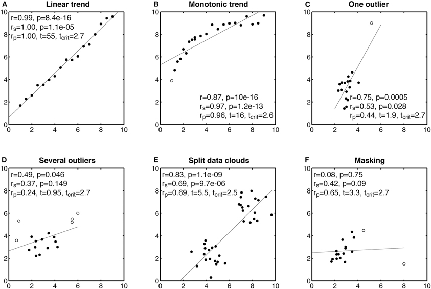
Figure 1. Examples of Pearson and Spearman correlations. In each subplot, r is Pearson correlation, r_s is Spearman correlation, and r_p is a skipped correlation. Potential univariate and bivariate outliers are marked by circles and other points marked by disks. A skipped correlation is significant if t is larger than t_crit.

Pearson correlation can also be extremely sensitive to outliers. For instance, in Figure 1C, a single outlier influences the results. Without looking for outliers, one would conclude that there is a significant association between the two variables. This conclusion is, however, unjustified by the data, because most of the points are clustered together with no obvious relationship. This is a critical problem, particularly true with Pearson correlation, but also all the techniques that rely on an ordinary least square solution: one badly positioned point can have a dramatic influence on the results (Hubert et al., 2008). Spearman correlation is less sensitive to outliers than Pearson, and in this case indicates a much weaker correlation. The skipped correlation flags the outlier successfully, and suggests the existence of a weak, not statistically significant, correlation. In other cases, there might be more than one outlier, and it is important to use a correlation technique that can handle a large proportion of extreme data points. In Figure 1D, most of the data are concentrated in a homogenous cloud of points. Two other groups of points, two to the left, and three to the right of that main cloud have been flagged as outliers. These extreme points influence Pearson correlation, and using this technique we would again conclude that there is a significant association between the two variables. However, Spearman and the skipped correlation return non-significant results.

Instead of few outliers, data can sometimes be organized in two clouds of points, such that no point can be categorized as outlier (Figure 1E). Because of this special structure, all correlation techniques return strong estimates. However, when the data are split into two clouds, it is likely that we are dealing with two groups of data. Without evidence that some observations would fall along the line between the two clouds, it seems inappropriate to apply correlation. Finally, one should keep in mind that outliers can not only create false correlations, but can also hide existing correlations, a phenomenon known as masking (Figure 1F). In that last example, a strategically placed outlier blinds Pearson to a true correlation. Spearman is less fooled than Pearson by the outlier and a skipped correlation detects it. Examples from Figure 1 are not such extreme caricatures, as examples from the literature described in the next section suggest. However, they have the advantage of being simulated data, in which we control the parameters. In research, it is more difficult to tease apart outliers from real data points. Because in many situations, researchers have weak or no priors, it seems safer to use robust outlier detection techniques rather than risking reporting and interpreting erroneous correlations.

Analyses of Published Results

We now illustrate how using Pearson correlation can potentially lead to inaccurate inference, by drawing examples from 55 articles published in 16 journals (Cerebral Cortex, Current Biology, European Journal of Neuroscience, International Journal of Psychophysiology, Journal of Cognitive Neuroscience, Journal of Neuroscience, Nature, Nature Neuroscience, Neurobiology of Aging, NeuroImage, Neuron, Neuropsychologia, Proceedings of the National Academy of Sciences of the United States of America, Psychological Science, Psychophysiology, Science). Our goal was not to systematically survey the literature, but rather to show that mainstream journals, from high-impact general outlets to specialty journals publish papers containing potentially inaccurate analyses. Our re-analyses of these data does not provide an ultimate description of the truth, especially because the true population associations are unknown and the estimations are complicated by small sample sizes. Instead, our analyses suggest that robust techniques can provide different results from those obtained with Pearson correlation alone, thus raising the possibility of spurious associations being published.

Data were obtained directly from the authors of two papers, and were extracted from published figures using the mac software GraphClick version 3.0 (Arizona Software, 2008) for the other papers. We did not obtain data from all the figures from all the studies: in fact several surveyed studies do not show data at all, preventing readers from assessing their correlations. Other studies had too poor figure quality, for instance with unreadable or unticked axes or contained several mistakes. For all data-sets we did analyse, we replicated very closely the published Pearson or Spearman correlations. Because of variability in image quality, results did differ slightly in few cases but these small variations have no impact on the key points of this article. Pearson and Spearman correlation were computed using the corr() function in Matlab R2011a. Confidence intervals for these correlation values were estimated using a percentile bootstrap (Wilcox, 2005). Skipped correlations were computed using Wilcox's skipped correlation functions in the R environment (R Development Core Team, 2011). In particular, we used (1) the scor() function with options corfun = spear, for Spearman correlation, and (2) cop = 2, so that the location estimator was based on the MCD. The scor() function calls the outpro() function, with option MM = T, so that the MAD estimator (Median Absolute Deviation to the median) was used to reject outliers.

Effects of Outliers on Correlations

Plots A, B, and C in Figure 2, and Figures A1–A3, present examples from the literature in which one or several outliers might have introduced false correlations. Although some of these outliers might seem questionable, particularly given the small sample sizes, it can be very difficult to identify multivariate outliers by eye-balling the data, by contrast with marginal outliers (Hubert et al., 2008). In the examples presented here, Pearson correlation suggests the existence of a significant association between two variables, whereas visual inspection of the bivariate distributions suggests that most data points are clustered together, without obvious linear association among themselves. Few data points, flagged by the robust multivariate outlier detection technique presented in the previous section differ from the bulk of the data, potentially causing the association. Indeed, after removing these outliers, none of the correlations presented in these figures are significant. In some cases, even without removing outliers, Spearman correlation was not significant. In other situations, after removing outliers, significant correlations emerged, or became significantly stronger than they were in the presence of outliers (Figure 2D, Figure A4). This illustrates a very important point: a non-significant correlation cannot be used to conclude that there is no association in the data, not just because of the null hypothesis framework, but because of power issues and the impossibility of testing all possible non-linear relationships with one technique. Thus, based on our analyses, we cannot conclude with certainty that no association exists between variables tested in those studies. However, we can conclude that, given the data at hand, there was no sufficient evidence to suggest the existence of a linear or monotone association.

FIGURE 2

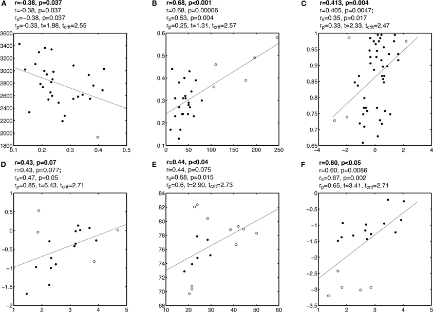
Figure 2. Questionable correlations observed in published articles. Each subplot contains a reproduction of the original data and regression line. Outliers are marked by circles and other points marked by disks. Analyses are reported above each subplot: the first line contains the correlation reported by the authors; the second line contains the Pearson correlation r from our analyses; the third line contains Spearman correlation r_s; the fourth line contains the skipped correlation r_p. Subplots A, B, C illustrate correlations that could be due to outliers. Subplot D illustrates a potential case of masking. Subplots E and F show the potentially incorrect use of correlation for what could be split data clouds.

Split Data Clouds

In some situations, the bivariate distribution suggests that the data, rather than being organized in one coherent cloud, are split into different groups (Figure 2E and 2F, Figure A5). In these cases, the joint distribution is bimodal and a correlation analysis might not be appropriate because the data clouds would be better studied independently. One such scenario could lead to the Simpson's paradox: a correlation present in different groups is reversed when the groups are combined (Simpson, 1951; Blyth, 1972). Although we have not seen such a case, plot E in Figure 2 provides a puzzling example, in which most of the points are organized along a vertical line, but the outlier detection method revealed potentially several groups. This illustrates that one should be cautious in assuming that data belong to one homogeneous distribution because it is possible that the random sample of subjects is inhomogeneous. In turn, it can be informative to consider subgroups of subjects, but in doing so there is a strong risk of increasing the false positive rate by changing the analyses after looking at the data. In doubt, as in the case of Figure 2E, it might be better not to compute any correlation at all and to attempt an independent replication of the results (see below).

Data (Mis)Interpretation

Strength of Evidence

Many journals encourage researchers to report estimates of effect sizes in addition to statistical significance tests. In general, it is also recommended to produce confidence intervals of those estimates. Because correlation coefficients are on a standardized scale, they represent directly the strength of the effect. However, to assess this strength, it is essential to report the error associated with it. Regrettably, we did not find a single publication in which the authors explicitly considered confidence intervals and the coefficient of determination (r²) in the interpretation of their results. Instead, most papers gave the impression that correlations were classified in one of two categories based on their p values. Correlations with p values inferior to 0.05 tended to be deemed interesting to report, and occasionally low p values were used to suggest the existence of strong, reliable, or robust effects. Correlations with p values larger than 0.05 were either dismissed, or occasionally described as trends or marginally significant effects.

Beyond the classic problems associated with interpreting p values and null hypothesis testing (Goodman, 1999; Wagenmakers, 2007; Miller, 2009; Rousselet and Pernet, 2011; Wagenmakers et al., 2011; Wetzels et al., 2011), the presentation of correlation results as all or nothing, without consideration for effect sizes and confidence intervals is not satisfactory. Let us consider the example in Figure 2A. Because both Pearson and Spearman are statistically significant, an unfounded conclusion could be “variable A predicts variable B (r = −0.38, p < 0.05).” In contrast, the strength of the effect (the coefficient of determination r² = 14% of variance explained) suggests a modest association, as also depicted by the scatterplot. It might be difficult to give a direct interpretation of the strength of a correlation because of the complex nature of and potential biases in analyzing brain imaging data (Yarkoni, 2009). Nevertheless, a more accurate conclusion could be “Pearson correlation suggests that variable A accounts for 14% of the variance in variable B.” In addition, a percentile bootstrap confidence interval revealed a large uncertainty about r [−0.69 −0.02], which implies that this correlation should be interpreted with caution. This example illustrates the importance of effect size and sampling error in the interpretation of correlations. Finally, if effects are small, or new, or unexpected, or any combination of those, it seems appropriate that the burden of evidence lies with the authors, who should replicate their own results in order to convince readers (e.g., Forstmann et al., 2010).

Significance Fallacy

Multiple correlations are often performed between one behavioral measure and several brain areas, with the goal of identifying the brain area with the strongest correlation. Only few of the papers we surveyed provided quantitative tests of the difference between correlations. Instead, most authors described implicitly or explicitly a significant correlation as being different from a non-significant correlation, a statistical fallacy covered in more details by (Nieuwenhuis et al., 2011). To compare correlations between brain areas, a formal test between correlation coefficients must be performed. This is best achieved using a percentile bootstrap test of the differences between correlations, with special adjustments in the case of Pearson correlation (Wilcox, 2009, 2012).

Multiple Testing Issue

Accurate correction for multiple comparison is not that easy to achieve, and there is no one size fits all procedure (Wilcox, 2005). It is nevertheless alarming that in the sample of articles we analyzed, very few authors attempted to correct for multiple comparisons, or even mentioned multiple comparisons as a moderating factor in their interpretations. We found many publications that reported over 10 correlations (36 and 40 correlations were the highest numbers we found) with no consideration for multiple testing. In fact, given the number of correlations with p values just below 0.05, controlling for as little as 2 or 3 correlations would make many correlations not significant. In addition to this problem, several authors used unjustified one-tailed tests, or even described non-significant correlations alongside significant correlations, as if they were significant and regardless of effect sizes. Unless justified, authors should thus (1) use two-tailed tests and (2) adjust their p value cut-off to control for multiple comparisons.

Conclusion

We have illustrated several problems associated with the lack of robustness of Pearson correlation and its use in the brain imaging literature. From our own scrutiny of the literature, it seems that many journals regularly publish weak, false, or hidden correlations. On the basis of Pearson correlations, many authors tend to conclude about the existence or non-existence of significant relationships between two variables, sometimes leading to maybe unwarranted conclusions. This problem is aggravated by the lack of consideration for effect sizes and sampling errors, the lack of adequate testing, and the lack of correction for multiple comparisons. All of these problems can be addressed by following simple recommendations, including, but not limited to: (1) looking carefully at the data to detect possible marginal outliers and evaluate the type of association (linear, monotone, non-linear); (2) using robust techniques to detect univariate and multivariate outliers, such as projection techniques in conjunction with the MCD; (3) analyzing the shape of the distributions (univariate and joint); (4) comparing standard correlations to robust correlation techniques to evaluate the impact of outlier removal; (5) correcting for multiple comparisons; (6) putting emphasis on effect sizes and robust confidence intervals. The adoption of better standards will help shift the emphasis away from p < 0.05, to focus on quantitative predictions about the results and comparisons across studies.

Conflict of Interest Statement

The authors declare that the research was conducted in the absence of any commercial or financial relationships that could be construed as a potential conflict of interest.

References

Barnett, V., and Lewis, T. (1994). Outliers in Statistical Data. Chichester: Wiley.

Blyth, C. R. (1972). Simpsons paradox and sure-thing principle. J. Am. Stat. Assoc. 67, 364.

Forstmann, B. U., Anwander, A., Schafer, A., Neumann, J., Brown, S., Wagenmakers, E.-J., Bogacz, R., and Turner, R. (2010). Cortico-striatal connections predict control over speed and accuracy in perceptual decision making. Proc. Natl. Acad. Sci. U.S.A. 107, 15916–15920.

Pubmed Abstract | Pubmed Full Text | CrossRef Full Text

Goodman, S. N. (1999). Toward evidence-based medical statistics. 1, The P value fallacy. Ann. Intern. Med. 130, 995–1004.

Pubmed Abstract | Pubmed Full Text

Hubert, M., Rousseeuw, P. J., and van Aelst, S. (2008). High-breakdown robust multivariate methods. Stat. Sci. 23, 92–119.

Iglewicz, B., and Hoaglin, D. C. (1993). How to Detect and Handle Outliers. Milwaukee, WI: ASQC.

Lazic, S. E. (2010). Relating hippocampal neurogenesis to behavior: the dangers of ignoring confounding variables. Neurobiol. Aging 31, 2169–2171; discussion 72–75.

Pubmed Abstract | Pubmed Full Text | CrossRef Full Text

Miller, J. (2009). What is the probability of replicating a statistically significant effect? Psychon. Bull. Rev. 16,617–640.

Pubmed Abstract | Pubmed Full Text | CrossRef Full Text

Nieuwenhuis, S., Forstmann, B. U., and Wagenmakers, E. J. (2011). Erroneous analyses of interactions in neuroscience: a problem of significance. Nat. Neurosci. 14, 1105–1107.

Pubmed Abstract | Pubmed Full Text | CrossRef Full Text

R Development Core Team, (2011). “R: A language and environment for statistical computing,” R Foundation for Statistical Computing, Vienna, Austria. ISBN 3-900051-07-0. URL http://www.R-project.org/

Rousseeuw, P. J. (1984). Least median of squares regression. J. Am. Stat. Assoc. 79, 871–880.

Rousseeuw, P. J., and Leroy, A. M. (1987). Robust Regression and Outlier Detection. New York, NY: Wiley.

Rousseeuw, P. J., and van Driessen, K. (1999). A fast algorithm for the minimum covariance determinant estimator. Technometrics 41, 212–223.

Rousselet, G. A., and Pernet, C. R. (2011). Quantifying the time course of visual object processing using ERPs: it's time to up the game. Front. Psychol. 2:107. doi 10.3389/fpsyg.2011.00107

Pubmed Abstract | Pubmed Full Text | CrossRef Full Text

Simpson, E. H. (1951). The interpretation of interaction in contingency tables. J. R. Stat. Soc. B 13, 238–241.

Vul, E., Harris, C., Winkielman, P., and Pashler, H. (2009a). Puzzlingly high correlations in fMRI studies of emotion, personality, and social cognition. Perspect. Psychol. Sci. 4, 274–290.

Vul, E., Harris, C., Winkielman, P., and Pashler, H. (2009b). Reply to comments on “puzzlingly high correlations in fMRI studies of emotion, personality, and social cognition”. Perspect. Psychol. Sci. 4, 319–324.

Wagenmakers, E. J. (2007). A practical solution to the pervasive problems of p values. Psychon. Bull. Rev. 14, 779–804.

Pubmed Abstract | Pubmed Full Text

Wagenmakers, E. J., Wetzels, R., Borsboom, D., and van der Maas, H. L. (2011). Why psychologists must change the way they analyze their data: the case of psi: comment on Bem (2011). J. Pers. Soc. Psychol. 100, 426–432.

Pubmed Abstract | Pubmed Full Text | CrossRef Full Text

Wetzels, R., Matzke, D., Lee, M. D., Rouder, J. N., Iverson, G. J., and Wagenmakers, E. J. (2011). Statistical evidence in experimental psychology: an empirical comparison using 855 t tests. Perspect. Psychol Sci 6, 291–298.

Wilcox, R. (2004). Inferences based on a skipped correlation coefficient. J. Appl. Stat. 31, 131–143.

Wilcox, R. R. (2005). Introduction to Robust Estimation and Hypothesis Testing. New York, NY: Elsevier Academic Press.

Wilcox, R. R. (2009). Comparing Pearson Correlations: dealing with heteroscedasticity and nonnormality. Commun. Stat. Simul. Comput. 38, 2220–2234.

Wilcox, R. R. (2012). Introduction to Robust Estimation and Hypothesis Testing. Amsterdam; Boston, MA: Academic Press.

Wilcox, R. R., and Muska, J. (2001). Inferences about correlations when there is heteroscedasticity. Br. J. Math. Stat. Psychol. 54, 39–47.

Pubmed Abstract | Pubmed Full Text

Yarkoni, T. (2009). Big correlations in little studies: inflated fMRI correlations reflect low statistical power, commentary on Vul et al. (2009). Perspect. Psychol. Sci. 4, 294–299.

Pubmed Abstract | Pubmed Full Text | CrossRef Full Text

Appendix

FIGURE A1

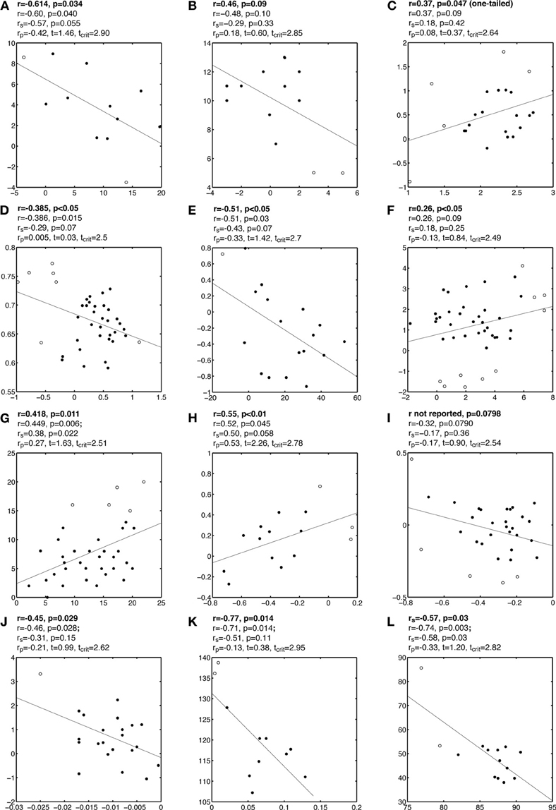
Figure A1. Examples of false correlations potentially due to outliers. Each subplot contains a regression line and a scatterplot with outliers marked by circles and other points marked by disks. Analyses are reported above each subplot: the first line contains the Pearson or Spearman correlation reported by the authors; the second line contains the Pearson correlation we obtained; the third line contains Spearman correlation r_s; the fourth line contains the skipped correlation r_p.

FIGURE A2

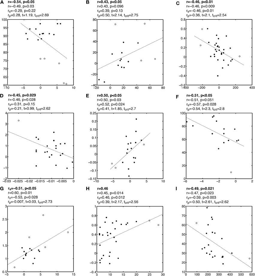
Figure A2. Examples of false correlations potentially due to outliers. See Figure A1 caption for details.

FIGURE A3

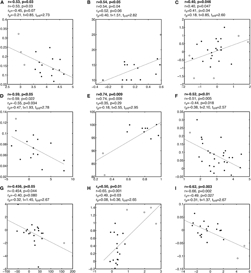
Figure A3. Examples of false correlations potentially due to outliers. See Figure A1 caption for details.

FIGURE A4

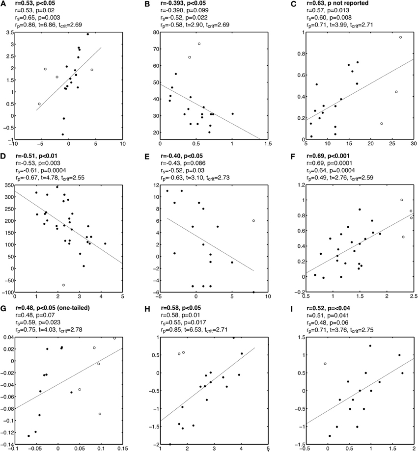
Figure A4. Examples of correlations potentially masked by outliers. See Figure A1 caption for details.

FIGURE A5

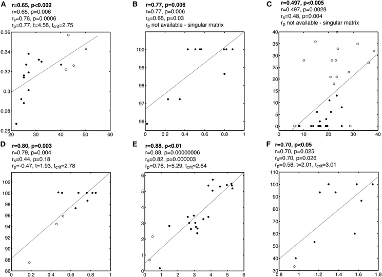
Figure A5. Examples of false correlations potentially due to split data clouds. See Figure A1 caption for details.