Uncertainties in early-stage capital cost estimation of process design – a case study on biorefinery design

Introduction

Economic growth leads to the development of processes and activities that are highly energy dependent. The use of fossil fuels as the main energy resource has many issues including long-term availability, supply security, and price volatility as well as environmental impact and climate change effects. Biorefineries arise potentially as a promising, clean, and renewable alternative to partly replace fossil fuels for both production of energy and chemicals.

The design of a biorefinery is, however, a challenging task. First, several different types of biomass feedstock, and many conversion technologies, can be selected to match a range of products, and therefore, a large number of potential processing paths are available. Secondly, being based on biomass (natural feedstock), the economic and environmental viability of these processes is deeply dependent on local factors such as land use and availability, weather conditions, national or regional subsidies, and regulations. Thus, designing a biorefinery requires a detailed screening among a set of potential configurations to identify the most suited option that satisfies a wide set of conditions. A detailed evaluation among process alternatives is required for a robust decision-making and it demands a substantial amount of information (e.g., conversions and efficiencies), which is both time and resource intensive. In order to overcome the aforementioned challenges, a decision support toolbox including methods and tools for early-stage process design and synthesis was developed in an earlier study (Cheali et al., 2014). An important aspect of the methodology is data collection and uncertainty assessment of the cost data used for cost estimation in particular.

Cost estimation is one of the major challenges of chemical and biochemical process design. The cost estimation (including fixed and variable cost) during each stage of the project design (concept screening, preliminary study, budget authorization, budget control, and construction) is different since the quality and quantity of the information available in the successive stages of the project life cycle is different (Towler and Sinnott, 2013). The Association of the Advancement of Cost Estimating International (AACE International) classifies the capital cost estimation into five classes, according to the level of accuracy and the purpose of the estimation in specific parts of the project life cycle (Table 1).

TABLE 1

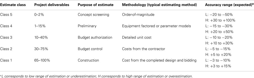
Table 1. Cost estimate classification matrix for the process industries [adapted from Christensen and Dysert (2011)].

Class 5, Concept Screening (Order-of-Magnitude)

This class is based on the cost data and the capacity from similar plants, and it is usually used for initial feasibility studies and for screening purposes. Class 4, preliminary (study of feasibility). This class mainly uses factors for the estimation, relying on so-called factored estimation methods. This method is based on material and energy balances as well as types and size of major equipment. It is used to make a rough screening among the design alternatives. Class 3, detailed design (budget authorization or definitive estimate). The project control estimate method is based on the approximate sizes of the major equipments; it is used for the authorization of project funds. Class 2, contractor estimate (budget control or detailed estimate). The quotation or contract estimate is based on the front-end engineering design (FEED) including the complete quotation of the equipment. This cost estimation is very detailed and is generally used to make a fixed price contract and to control the project cost. Class 1, construction (check estimates). The bid or tender estimate is based on the completed design and concluded negotiation on procurement.

The cost estimation has a significant impact on the project life cycle as presented in Figure 1. At the early-stage, the possibility to change the design (black full line) is the highest with the lowest cost (black dashed line). Therefore, the main motivation for investing in such a detailed analysis and treatment of cost data uncertainties at the early-stage of process design is simply that this stage has the highest impact on the overall project economics and feasibility considering the typical life cycle of a project (to move the red dashed line to the blue one). Hence, since increased investment of time and resources is required by these analyses, it will mean that the project cost will be high at the beginning of the project life cycle. However, the advantage is that the improved quality of decisions that is achieved thanks to these rather detailed early-stage analysis efforts will translate to reduced project cost during the later stages of the project life cycle.

FIGURE 1

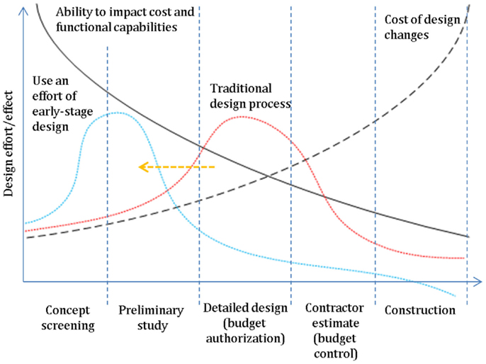
Figure 1. The design effort and impact on the project development [adopted from Towler and Sinnott (2013)].

In this contribution, we perform an in-depth analysis of the issues and challenges related to performing cost data estimation, and we develop methods and tools to properly address these issues in order to provide a robust decision-making platform for process synthesis and design. An assessment of the uncertainties of early-stage cost estimation methods will be performed. In particular, four standard models for cost estimation during the early-stage were considered for the analysis, and will be explained in the next section. Two different situations are considered for the uncertainty characterization and the cost estimation methods: (i) when historical cost data are available: the uncertainties of the cost estimation were obtained from regression analysis using the bootstrap regression technique. (ii) When cost data are not available: the Monte Carlo technique in combination with expert review of uncertainties is used.

The paper is organized as follows: (i) the methodology proposed for uncertainty characterization and estimation is introduced; (ii) the uncertainty estimation results are presented and the comparison among early-stage cost estimation methods is presented and discussed using bioethylene production as motivating example; and (iii) the impact of uncertainties in cost estimation on process synthesis and design is analyzed and discussed.

Materials and Methods

Cost Estimation Methods

Estimating the manufacturing costs of a new product/process during early-stage design can provide a good indication of the project’s economic viability (Christensen and Dysert, 2011). Early estimates generally used for conceptual screening have the purpose of allowing businesses to assign the most suitable resources and new/different alternatives (feedstock, technologies, or products) with respect to the defined specification. Anderson (2009) reported the methods to estimate three main cost components accordingly: (i) Variable cost. A good and insightful resource of relevant information (prices and availability) about the raw materials, and has a significant impact. If relevant information cannot be found, the risk related to this lack of information should be quantified using uncertainty analysis. The utility costs can be estimated using a rule of thumb approach (e.g., 2% of capital investment). (ii) Capital investment. The capital investment can be estimated using the order-of-magnitude or the Viola method, which requires only information about capacity and capital investment for similar existing technologies. If both the type and number of unit operations are known, the relative factor regarding each unit operation is applied further to refine the results. The depreciation can be estimated rapidly as well using the ratio of capital investment and the product of project lifetime and production rate. (iii) Other fixed costs (e.g., labor cost, maintenance). The factor-based rule of thumb is used for estimating the other fixed costs. In addition to the above, there are a variety of other estimation methods reported in the literature (Petley, 1997). Those, that use the recorded capacities and investment cost, are called exponent estimates. Those that use factors to multiply equipment costs to generate an overall investment cost are called factorial estimates. Those that use the plant parameters and functional units known in the early-stage design are called functional unit estimates. Those that use the production profit to estimate the overall production cost are called pay-back method. In this study, the four mentioned methods of early-stage cost estimation are used. These methods require different types of information, and therefore the results using different cost estimation methods will be compared and discussed.

Model 1: order-of-magnitude estimates (production rate and investment of the existing plant)

Exponent estimates are used in the early-stage design. The required capital cost is estimated by scaling the known investment cost corresponding to the capacity of an existing manufacturing plant (Eq. 1). This requires no complete design information. The value of the exponent (n) in Eq. 1 varies between 0.5 and 1 depending on the type of manufacturing process, as explained in Table 2.

TABLE 2

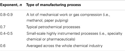
Table 2. The range of exponents typically used in the exponent based cost estimation methods (Towler and Sinnott, 2013).

Model 1,

$\begin{array}{llll}\hfill & \left(\begin{array}{c}\text{Capital cost of}\\ \text{the NEW\hspace{0.17em}plant},C_2\end{array}\right)=\frac{\left(\begin{array}{c}\text{Capital cost of}\\ \text{the OLD\hspace{0.17em}plant},C_1\end{array}\right)}{{\left(\begin{array}{c}\text{Capacity of}\\ \text{the OLD\hspace{0.17em}plant},S_1\end{array}\right)}^{\text{exponent}}}\times {\left(\mathrm{Capacity\hspace{0.17em}\hspace{0.17em}of\hspace{0.17em}\hspace{0.17em}the\hspace{0.17em}\hspace{0.17em}NEW\hspace{0.17em}\hspace{0.17em}plant,\hspace{0.17em}\hspace{0.17em}}{S}_2\right)}^{\left(\mathrm{exponent},n\right)};& \hfill & \\ \hfill & \frac{\left(\mathrm{Capital\hspace{0.17em}\hspace{0.17em}cost\hspace{0.17em}\hspace{0.17em}of\hspace{0.17em}\hspace{0.17em}the\hspace{0.17em}\hspace{0.17em}OLD\hspace{0.17em}\hspace{0.17em}plant,\hspace{0.17em}\hspace{0.17em}}{C}_{\mathrm{1}}\right)}{{\left(\mathrm{Capacity\hspace{0.17em}\hspace{0.17em}of\hspace{0.17em}\hspace{0.17em}the\hspace{0.17em}\hspace{0.17em}OLD\hspace{0.17em}\hspace{0.17em}plant,\hspace{0.17em}\hspace{0.17em}}{S}_{\mathrm{1}}\right)}^{\left(\mathrm{exponent},n\right)}}=a\end{array}$ (1)

It is important to note that when there are insufficient data available, n = 0.6 can be used for a rough estimation. This case is commonly referred as the six-tenths rule method. This approach refers to the economy of scale, meaning that increasing capacity of the plant decreases unit marginal production cost. The disadvantage of this method is the requirement of having information available about the capacity and investment data of similar plants. Therefore as well, this method can be particularly problematic for new processes. This method has been further developed by estimating the cost of the main equipment instead of the investment of the entire plant (Garrett, 1989). Using this method for estimating the cost during the R&D phase, the typical accuracy for chemical processes has been found by Uppal and Gool (1992) to be ±40%. Of course, it could be better or worse depending on the design criteria defined.

Model 2: Bridgewater’s methods (production rate, number of functional units, and conversion fraction)

Factorial estimates were first introduced by Lang (1947) to estimate the investment cost by multiplying the equipment costs with a factor (Eq. 2).

$C=f\times E$ (2)

where C is the capital cost, $; f is the factor (3.10 for solid processing; 3.63 for combined solid and fluid processing; and 4.74 for fluid processing); E is the equipment cost, $). The equipment costs can be determined from the quotations of vendors, from published data or by estimation using design information. The overall factors can be divided into different categories, i.e., for foundations, supports, insulation, installation, piping and contractors, and engineering expenses. Cran (1981) suggested using a universal factor of 3.45 instead of classifying the plants into three types as shown above. Miller (1965) reported that the factors depend on the size of the equipment, the material of construction, and the operating pressure resulting in the effect on the average cost of each piece of equipment in the process. The factorial method has been developed by many authors. However, this is a complicated method considering that there are many types of components of several manufacturers related to each process (process type, equipment, functional units, capacity, piping, and instrumentation). Moreover, the companies generally develop their own values taking into account their specific requirements resulting in a wide range of the factors.

Alternatively, when the cost data for a similar process are not available, then, the order-of-magnitude estimate can be used with some modifications by employing the different plant sections or functional units. For example, experienced engineers provide a quick guideline for many petrochemical processes by considering that 20% of the investment is for the reactor and 80% is for the distillation and product separation. This alternate approach, called Functional unit estimates uses the process parameters and the functional units during the early-stage design to predict the investment cost instead of using the equipment cost and factors as in the Factorial estimates method. The method has been derived by a statistical analysis of existing plants for determining the sequence of significant process steps (functional units). The method was introduced by Wessel (1953) who used the number of processing steps to calculate the labor costs. The functional units separate the process into these processing steps where the material compositions are significantly changed, for instance, a reaction or separation. The equipment cost (E) Eq. 2 of Factorial estimates, is replaced by the number of functional units (U_N) as presented in Eq. 3.

$C=F\times \left(\mathrm{IEC}\right)=F\times \left(U_N\times {\left[\frac{Q}{10}\right]}^{0.6}\times 30000\right)$ (3)

where C is the capital cost in 1954 ($); F is the Chilton factor to allow for piping, instrumentation, facilities, engineering, construction, and capacity; IEC is installed equipment cost ($); Q is the capacity (tons per year).

Bridgewater’s method (Bridgewater and Mumford, 1979) has been developed and applied for early capital cost estimation using (capacity/overall conversion) as the capacity together with the functional units as presented in Eq. 4 and the recently developed models in Eq. 5, which are used as Model 2 for the analysis in this study.

$C=k\times U_N\times {\left[\frac{Q}{s}\right]}^x$ (4)

Model 2,

$\begin{array}{l}\hfill Q\ge 60000:C=4320\times U_N\times {\left[\frac{Q}{s}\right]}^{0.675};Q<60000:C=380000\times U_N\times {\left[\frac{Q}{s}\right]}^{0.3}\end{array}$ (5)

where C is the capital cost in 1992 (£); Q is the capacity (tons per year); k is a constant; x is an exponent. However, determining the value for the number of functional units U_N is a major challenge of this method due to the inconsistency of the definition of the functional units.

Model 3: pay-back method (production rate, raw material, and product price)

Apart from the general methods mentioned above, using the profit and production cost can also be applied for a rough cost estimation. The pay-back method (Eq. 6) estimates the plant cost by assuming that the company would be paid back within 3–5 years (average is 4 years, the first factor) of pay-back period, for a rough estimate of the plant cost. The net profit is then estimated by assuming that the raw materials costs represent 80–90% of the total annualized cost (TAC), resulting in the second factor of 1.2. It is important to note that this method is normally used under the assumption that the specific project will generate a reasonable return.

Model 3,

$\mathrm{Plant}\mathrm{cost}=4\times \left(\mathrm{product}\mathrm{sales}-1.2\times \mathrm{raw}\mathrm{material}\mathrm{cost}\right)$ (6)

Model 4: total cost of production method (production rate, raw material, and product price)

Total cost of production (TCOP) is simpler than the pay-back method using the raw material cost for estimating the annualized production cost. This method (Eq. 7) is normally applied for a large-scale production (>500,000 pieces per year). This method is a rule of thumb method assuming that the annualized capital cost is one-fifth of the total annualized production cost (including raw material cost, utility cost, and annualized capital cost).

Model 4,

$\begin{array}{ll}\hfill & \mathrm{Plant}\mathrm{cost}=\mathrm{project}\mathrm{life}\mathrm{cycle}\left(\mathrm{year}\right)\times \frac{\mathrm{TCOP}}{5};\mathrm{TCOP}=2\times \mathrm{raw}\mathrm{material}\mathrm{cost}\end{array}$ (7)

The methods reviewed above have been applied to many cases and provide a good guideline during the decision-making processes. However, when extrapolating to fundamentally different plants and processes, the accuracy of their estimation becomes challenged due to uncertainties in their assumptions/factors/parameter values.

Uncertainty Characterization and Estimation of Cost Data

In this step, the uncertainties involved in cost estimation are reviewed and analyzed. To this end, two different methods are presented dealing with two distinct situations: (a) cost data available: in this case, cost data are reported from prior experiences with plant construction and operations. In this case, the challenge is to estimate the parameters of the cost estimation model using the data and then to quantify the accuracy of the estimation using regression analysis; (b) cost data not available: this case refers to situations where new technology is developed, and hence there are no prior experiences or the technology in question is not mature. For this situation, the uncertainties can be characterized by using an expert judgment and peer review procedure (Sin et al., 2009). Once uncertainties have been defined, then the Monte Carlo technique can be used to propagate these uncertainties in the analysis. For the aforementioned purpose, a framework for characterizing the uncertainties of early-stage cost estimation is proposed and presented in Figure 2.

FIGURE 2

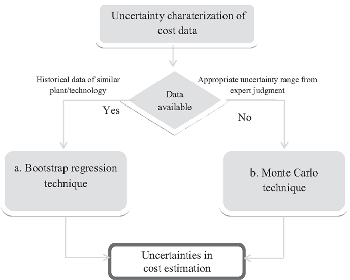
Figure 2. The simplified framework of uncertainty analysis for early-stage cost estimation.

Bootstrap Regression for Parameter Estimation

Bootstrap regression (Efron, 1979) is a method for assigning measures of accuracy (defined in terms of bias, variance, confidence intervals, etc.) to sample estimates. This technique allows estimation of the sampling distribution of almost any statistic using only very simple methods.

This method can be divided into three main steps: (i) Parameter estimation; (ii) Generation of synthetic data (bootstrap sampling); and (iii) Evaluation of the distribution of theta. The bootstrap theory is briefly explained in the following using a simple non-linear model (y_i = f_i (θ) + ε_i) as an example.

Parameter estimation. The actual data set D₍₀₎, “measures” a set of parameters θ_true. These true parameters are statistically realized as a measured data set D₍₀₎. The data set D₍₀₎ is known as the experimenter. The experimenter fits a model to the data by a minimization (i.e., using least squares; $\stackrel{⌢}{\mathrm{\theta }}:\mathrm{mi}{\mathrm{n}}_{\mathrm{}\mathrm{\theta }}{∥y-f\left(\mathrm{}\mathrm{\theta }\right)∥}^2$) or other techniques and obtains measured, fitted values for the parameters, θ₍₀₎.

Generate synthetic data (bootstrap sampling). In this step, the actual data set D₍₀₎ is then used to generate a number of synthetic data sets $(D_{(1)}^s,D_{(2)}^s,\dots ,D_{(Ns)}^s)$ using bootstrap sampling, i.e., random sampling with replacement technique. N_s indicate the total number of samples generated. Therefore, based on the given non-linear example, the bootstrap defines $\stackrel{⌢}{F}=\mathrm{mass}\frac{1}{\mathit{Ns}}$ as the sample probability distribution of $\stackrel{⌢}{\mathrm{\epsilon }}=(y_i-f_i(\widehat{\mathrm{\theta }}))$. Then, for the given $\stackrel{⌢}{F}$ and $\stackrel{⌢}{\mathrm{\epsilon }}$, the bootstrap sample is $y_i^{\ast }=f_i(\widehat{\theta })+{\mathrm{\epsilon }}_i^{\ast }$ where ${\mathrm{\epsilon }}_i^{\ast }$ is obtained using random sampling with replacement from the residuals $\stackrel{⌢}{\mathrm{\epsilon }}$.

Evaluate distribution of theta. For each data set, the same estimation procedure using least square method is performed giving a set of estimated parameters $({\text{θ}}_{(1)}^s,{\text{θ}}_{\text{(2)}}^s,\dots )$. The distribution of estimated values for each parameters $({\text{θ}}_{(1)}^s,{\text{θ}}_{\text{(2)}}^s)$ is plotted (e.g., histogram) for graphical analysis as well as for calculating the mean and standard deviation for each estimated parameter.

Monte Carlo technique

Uncertainty analysis using the Monte Carlo technique can be divided into four steps: (i) Input uncertainty characterization; (ii) Sampling; (iii) Model evaluations; and (iv) Output uncertainty analysis.

Input uncertainty. Based on historical data, experiences and realization, and the parameters, which are inconsistent, are generally selected as uncertain data. The parameters are then characterized by choosing a distribution function such as a uniform or normal distribution.

Sampling. The domain of uncertainty defined previously is sampled to generate a list of possible future scenarios, with equal probability of realization. In order to facilitate this task, and assure the quality of the sampling procedure (in terms of coverage of the uncertain space) the approach integrates a Latin Hypercube Sampling (LHS) based sampling technique with the rank correlation control method proposed by Iman and Conover (1982), in order to reflect the correlation between the uncertain parameters in the generated future scenarios.

Model evaluations. The generated Monte Carlo samples are then used as discretization points to approximate the probability integral, appearing in the objective function of optimization under uncertainty problems. The relationship between samples and outputs is established using a linear regression. In this regression, the parameter β_jk is the standardized regression coefficient (SRC) of the parameter j on output k; if β_jk has a negative sign, it means that a parameter j has a negative influence on the output k; if β_jk has a positive sign it indicates that a parameter has a positive influence on the output k; a high value of β_jk means a high impact on the output k. The sum of squares of the SRCs is equal to one $\left({\sum }_{j=1}^M{\mathrm{\beta }}_{\mathit{jk}}^2=1\right)$.

Output uncertainty. The results are then analyzed by using a non-parametric distribution function such as a cumulative distribution function (CDF), and frequentist statistics such as mean, variance, and percentile analysis, etc.

Motivating Example – Estimation of Uncertainty in Cost Data

Ethylene is an important and widely used intermediate in the chemical industries. The production of ethylene is used as a case study to highlight the uncertainties involved in cost estimation methods following the systematic methodology shown in Figure 3. The example consists of two parts: (i) bootstrap parameter estimation; (ii) Monte Carlo technique with an expert judgment of uncertainties.

FIGURE 3

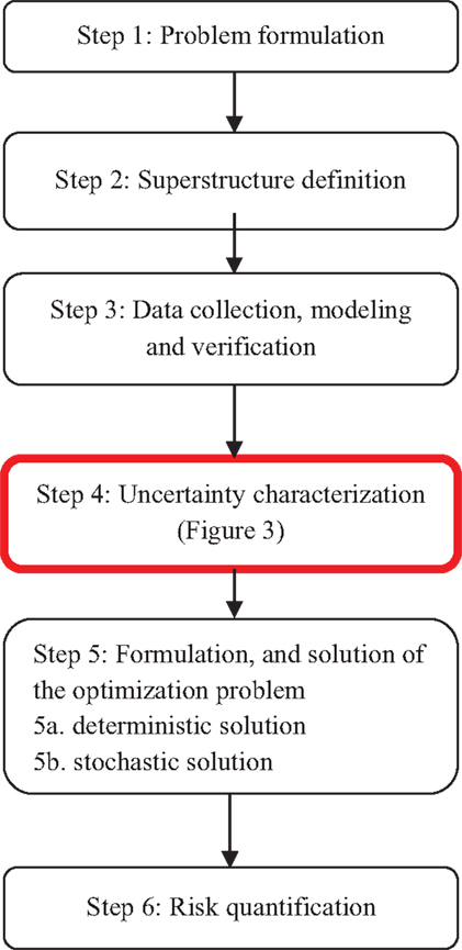
Figure 3. The highlighted step (Step 4) is expanded as presented in the methodology section (seeMaterials and Methods).

Bootstrap Regression for Parameter Estimation

Table 3 presents the capacity and investment cost of the existing plant, which can be used for estimating the capital investment using the order-of-magnitude method (Eq. 1). This information is reported annually by SRI Consulting, Chem Systems, NREL, or NETL. As presented in Table 3, there are five data points available, and the bootstrapping method is therefore applied.

TABLE 3

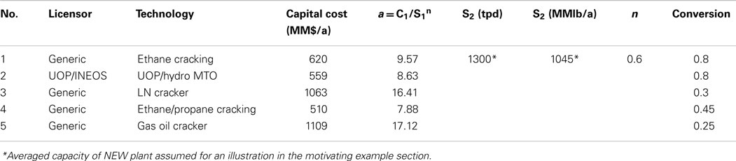
Table 3. Historical data for order-of-magnitude cost estimation (Towler and Sinnott, 2013).

Consequently, these data (Table 3) are regressed and characterized as the input parameters presented in Table 4. As shown in Table 4, the standard deviation is significant, and therefore, the parameter a is considered to be an uncertain parameter.

TABLE 4

Table 4. The input parameter for cost estimation using Model 1.

Early-Stage Cost Estimation – Monte Carlo Technique

When data of similar plants are unavailable, the suggestion from an expert can be used. In this section, the Monte Carlo simulation with expert judgment is used for uncertainty analysis on the cost estimation. Table 5 presents the input uncertain data for cost estimation methods, which are defined using the uncertainty factor with respect to the cost estimation accuracy in Class 5 (Table 1). To avoid any inaccuracy in the correlation between the parameters (the production rate, overall conversion, and the number of functional units), the uncertainty factor value, representing the uncertainties of the estimated capital cost, is used. The input data in Table 5 consist of two sections regarding two ranges of expert judgment: (i) lower range (underestimate), −50 to −20%; (ii) higher range (overestimate), +30 to +100%.

TABLE 5

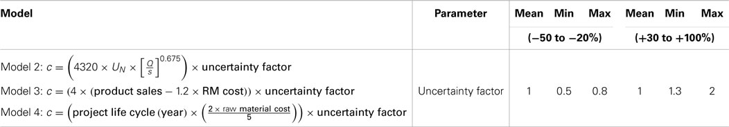
Table 5. The input parameters for three cost estimation models.

Results

The results of the different cost estimation methods are presented and compared in Table 6. Clearly, the estimation results obtained from different models yields significant differences. This motivating example confirms the significant impact on the selection of the methods for early-stage cost estimation. This impact on process synthesis and design will be analyzed and discussed in the next section.

TABLE 6

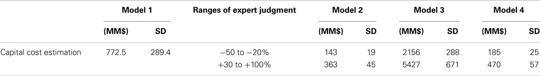
Table 6. The comparison of early-stage cost estimation for an ethylene production plant of 1300 tpd.

Process Synthesis and Design of Biorefinery: Impact of Uncertainties in Cost Estimation on the Decision Making

Process synthesis and design of a biorefinery during the early-stage has been developed earlier (Cheali et al., 2014) by applying a systematic framework for synthesis and design of processing networks. The capital investment is one of the key factors considered for techno-economic evaluation of alternatives. The framework (Figure 3) consists of six steps, which are briefly recalled here.

Step 1: Problem formulation (i.e., problem definition, superstructure definition, data collection, model selection, and validation).

Step 2: Superstructure definition.

Step 3: Data collection, modeling, and verification.

The problem in this study has been defined earlier. The biorefinery design networks resulting from earlier work are used here, and therefore, the development of the superstructure and the data collection/management were not repeated. However, it is necessary to present the superstructure (Figure 4). The objective function defined in this study was to maximize the operating profit (product sales – operating cost – annualized capital cost).

FIGURE 4

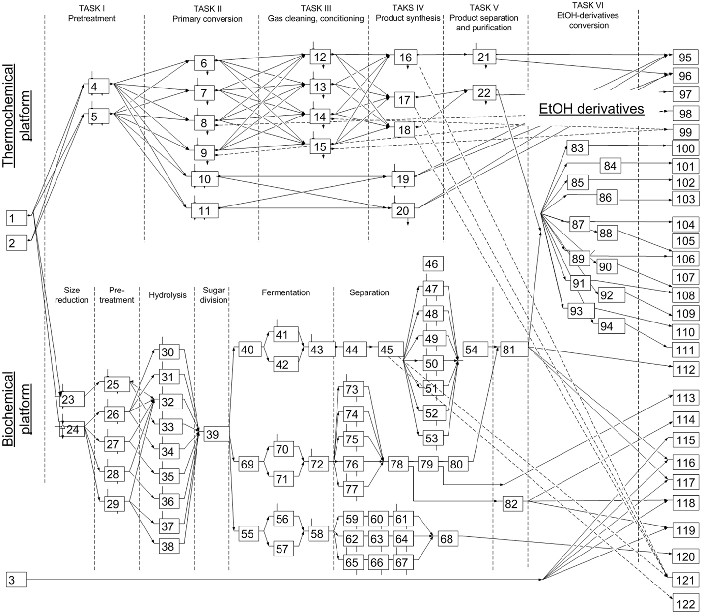
Figure 4. The superstructure of the biorefinery network extended with bioethanol based derivatives. Biomass feedstock (1–2); thermochemical conversion (4–22); biochemical conversion platform (23–82); ethanol-derivatives conversion (83–94); and bioproducts (95–122; FT-products, bioethanol, ethanol-derivatives, and electricity).

Step 4: Uncertainty characterization. In this step, the methodology presented earlier in Section “Materials and Methods” was applied to characterize the early-stage cost estimation. Since there is very little information on the existing plant producing bioethanol derivatives, the bootstrapping regression model could not be applied. The Monte Carlo approach with LHS was therefore applied instead.

Prior to any further analysis, it is important to note that there is only an overestimation scenario (+30 to +100%) that is presented in this context because it has a negative impact on the operating profit of the project. An underestimation scenario is presented in the Supplementary Material.

The input uncertainty for early-stage cost estimation is presented in Table 7. The parameters of each cost estimation method were selected as uncertain data, and they were characterized as a uniform distribution (mean/min/max) for two ranges of expert judgment with respect to the accuracy range presented in Table 1. The input uncertainties from Table 7 were then sampled for 200 scenarios.

TABLE 7

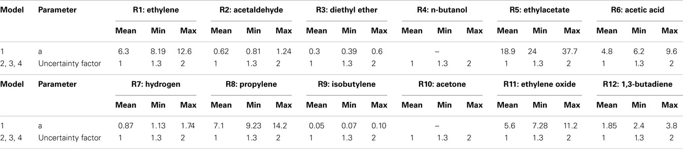
Table 7. Input uncertainties for early-stage cost estimation of ethanol derivatives for four cost estimation models.

Step 5: Formulation and solution of the optimization problem. 5a. Deterministic problem. The deterministic optimization problem is solved in this step. The result of this step is the deterministic solution of the optimal processing path, i.e., one optimal processing path on the basis of mean values representing the input data (Table 7). The top-five ranking of maximum operating profit is presented in Tables 8–11.

TABLE 8

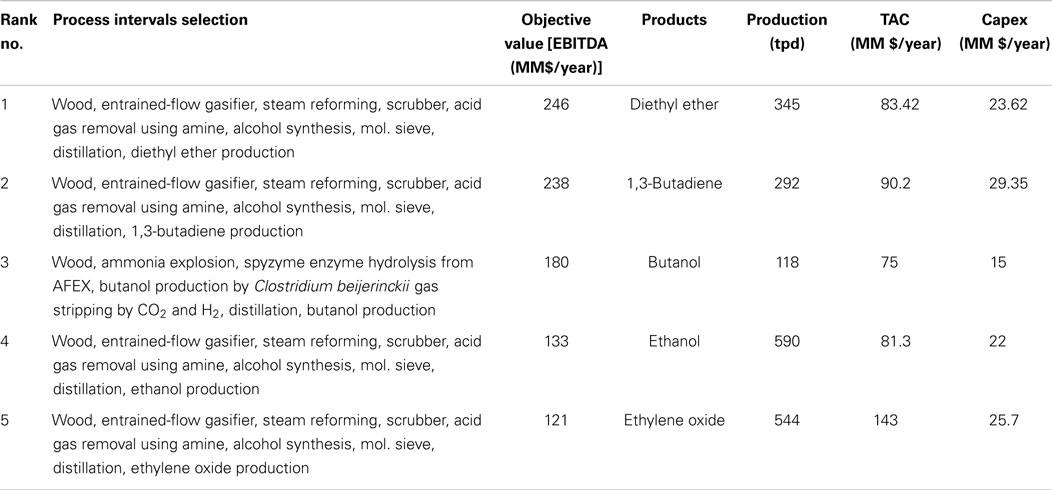
Table 8. Top-five ranking of the optimal solutions using Model 1 (+30 to +100%) for capital cost estimation (max EBITDA of producing ethanol derivatives).

TABLE 9

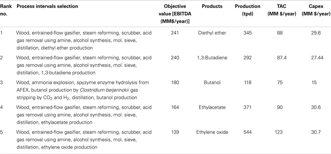
Table 9. Top-five ranking of the optimal solutions using Model 2 (+30 to +100%) for capital cost estimation (max EBITDA of producing ethanol derivatives).

TABLE 10

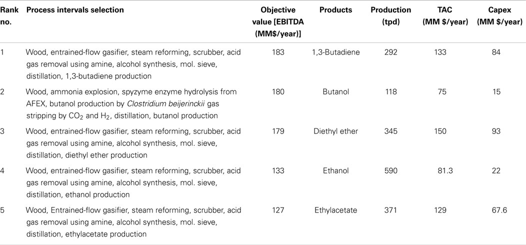
Table 10. Top-five ranking of the optimal solutions using Model 3 (+30 to +100%) for capital cost estimation (max EBITDA of producing ethanol derivatives).

TABLE 11

Table 11. Top-five ranking of the optimal solutions using Model 4 (+30 to +100%) for capital cost estimation (max. EBITDA of producing ethanol derivatives).

The results presented in Tables 8–11 show that there are slight differences in the results with respect to the identification of the optimal processing paths. Diethyl ether is predicted to be the most profitable using Model 1, Model 2, and Model 4 for estimating capital cost. On the other hand, 1,3-butadiene is predicted as being the most favorable product when using Model 3. Overall, the production of diethyl ether, 1,3-butadiene, and butanol are in the top-three ranking for every scenario.

5b. Uncertainty mapping. Instead of using a certain (mean) value as input data, the sampling results (200 samples generated in Step 4) from the uncertainty domain were used as the input data for the deterministic problem resulting in 200 optimal solutions.

The results (Table 12) are: (i) the probability distribution of the objective value; and (ii) the frequency of selection of the optimal processing path candidates under the generated uncertain samples. These identify the promising processing paths given the considered uncertainties.

TABLE 12

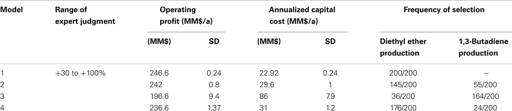
Table 12. Uncertainty mapping and analysis: frequency of selection with respect to 200 input uncertainty scenarios.

The results show that using Model 1, there were no changes of the optimal processing path compared to the deterministic solution. On the contrary, using Model 3, the production of 1,3-butadiene was more favorable confirming the results in Step 5a. Overall, the production of diethyl ether and 1,3-butadiene were reported to be the most favorable and profitable. The results in this step confirm the robustness of the deterministic solutions in Step 5a.

Step 6: Risk quantification. The results from Step 5a and Step 5b presented previously show that the production of diethyl ether and 1,3-butadiene are the most profitable/promising. Therefore, these two productions were further analyzed. In this step, EBITDA is converted (Eq. 8) into internal rate of return (IRR), which is an appropriate economic indicator for project evaluation. Figures 5 and 6 present the cumulative distribution of the % IRR related to diethyl ether and 1,3-butadiene production, respectively.

FIGURE 5

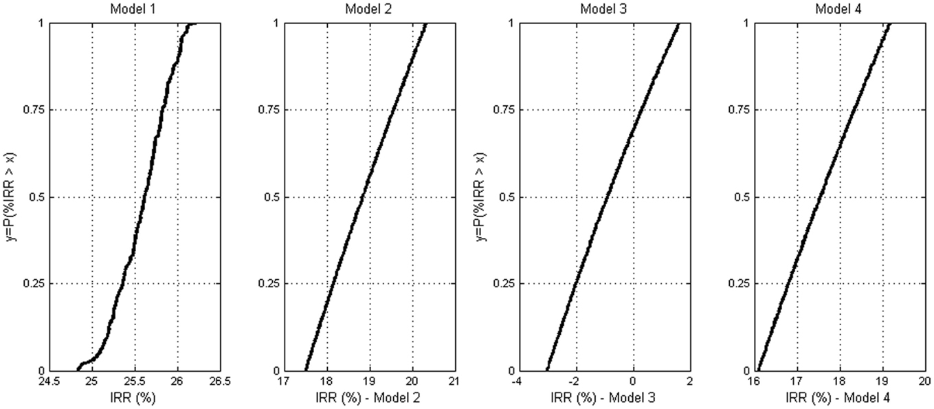
Figure 5. Diethyl ether production: the empirical cumulative distribution function (ECDF) of the IRR estimated from four estimation models.

FIGURE 6

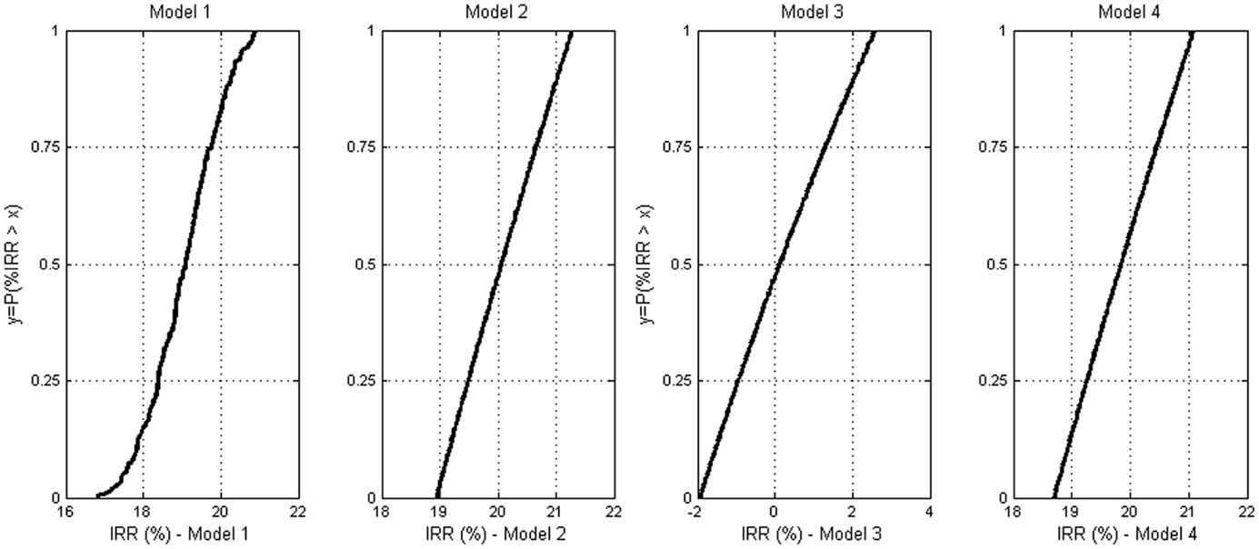
Figure 6. 1,3-Butadiene production: the empirical cumulative distribution function (ECDF) of the IRR estimated from four estimation models.

Risk analysis was also performed and analyzed based on the production of diethyl ether and 1,3-butadiene. Risk is defined as the probability (failed to achieve the target) times the consequence (the deviation from the target). In this study, the target is the IRR, which is estimated based on the certain value (mean) of the input parameter used for capital cost estimation. Table 13 presents the risks quantified based on the two production processes (diethyl ether and 1,3-butadiene), four cost estimation models, and the referenced estimation (no uncertainty considered).

TABLE 13

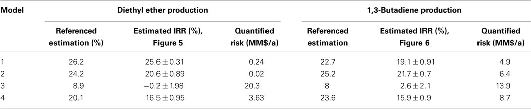
Table 13. Risk analysis of the production of diethyl ether and 1,3-butadiene.

As presented in Table 13, the risks quantified for diethyl ether production are lower compared to 1,3-butadiene production except for the case where Model 3 was used. The reason for this is that the price of diethyl ether is lower resulting in a lower operating profit and IRR. Moreover, Model 3 resulted in a significantly lower IRR compared to the results from the other models. Therefore, Model 3 should be considered as invalid.

Discussion

The comparison results show that different cost estimation methods lead to different results. This is because of the differences in the assumptions and the types of data used for the estimation. Therefore, the selection of the proper cost estimation method is critical.

Moreover, the results show that the uncertainty impact of cost estimation on the optimal processing paths is significant in the case study considered for the analysis. Hence, we conclude here that cost analysis cannot be based on a deterministic approach, but should be done using a probabilistic approach in which uncertainties are accounted for. Moreover, the Model 3 is found not to be preferable because the results are inconsistent compared to the other models. The underlying reason is attributed to the fact that the Model 3 is an indirect method that requires too much input information including the assumption of pay-back period, product sales, and raw material cost. Hence, Model 3 is more vulnerable to input uncertainties. On the contrary, the Model 4 – another indirect method, uses only one assumption (raw material cost) and provides more consistent results with the cost estimation obtained from direct methods, i.e., the Model 1 and Model 2.

In this study, IRR and EBITDA were used as economic indicators according to industrial practice (Towler and Sinnott, 2013). The results are expected to be the same as using net present value (NPV) due to the direct relation between IRR and NPV as presented in Eq. 8 (Towler and Sinnott, 2013).

$\begin{array}{ll}\hfill \mathrm{NPV}& =0-\mathrm{capital}\mathrm{investment}+\frac{\mathrm{EBITDA}}{{\left(1+\mathrm{IRR}\right)}^1}+\frac{\mathrm{EBITDA}}{{\left(1+\mathrm{IRR}\right)}^2}+\cdots +\frac{\mathrm{EBITDA}}{{\left(1+\mathrm{IRR}\right)}^{19}}+\frac{\mathrm{EBITDA}}{{\left(1+\mathrm{IRR}\right)}^{20}}\end{array}$ (8)

In engineering companies, the cost estimation is usually refined in each successive phase of the project. For example, in the detailed engineering phase, the cost estimation will be made based on the vendor information about pipes, tanks, etc. resulting in more accurate estimates compared to the rough estimation obtained at the early project stage using simple methods (the Model 1, 2, 3, and 4 as presented here). Hence as a future scope for further improving the accuracy of early-stage cost models, it is recommended to calibrate the model parameters against more accurate cost estimation models.

Overall the results in this study support the argument that while the early-stage assessment of the main cost components (capital investment and operating costs) is an approximation, these estimation results can still be useful for comparing and screening among alternatives (Anderson, 2009). Therefore, if the assumptions are reasonable, the process alternatives that are clearly economically infeasible can be identified early and removed from further analysis in subsequent project design stages.

Conclusion

An assessment of uncertainties in early-stage cost estimation of process synthesis and design of a biorefinery was studied and discussed. A systematic framework was applied consisting of a superstructure optimization based approach under uncertainty integrated with the proposed uncertainty characterization framework supporting the different types of data available (i.e., historical data from existing plants, an expert judgment). The comparison results from the case study on the process synthesis and design of the biorefinery problem showed that the results are different when using different cost estimation models. The Model 3 is found not to be favorable in this study because the results are inconsistent with the other models. Moreover, using the same methods including the uncertainties resulted in a significant impact on changing the selection of the processing paths. Therefore, the selection of early-stage cost estimation method is critical. Furthermore, the cost analysis cannot be based on a deterministic approach but should be evaluated by means of a probabilistic approach in which uncertainties are accounted for. It was found that the production of diethyl ether and 1,3-butadiene are the most economically profitable. These analyses provide useful information supporting the future development of biorefineries.

Nomenclature

Indexes
i	Components
Parameters
a	Constant used in order-of-magnitude method, is defined as CAPITAL COST of OLD plant divided by CAPACITY of OLD plant, with the exponent
n	Exponent used in order-of-magnitude method
f	Factor for estimating capital cost for factorial estimate
E	Equipment cost
IEC	Installed equipment cost
UN	No. of functional units
s	Overall conversion
x	Exponent used in Bridgewater’s method
Variables
C	Capital cost
Q	Production rate
S	Plant capacity used for order-of-magnitude method
D	Data set
Ns	Number of bootstrap samples
$\stackrel{⌢}{F}$	Sample probability distribution
ε	Measurement error
ykk	Selection of process intervals (binary)
wj,kk	Selection of a piece of the piecewise linearization (linear)
NPV	Net present value
Cn	Cash flow in year
Cn	Molar concentration of main product
Ncp	Number of co-products
MLI	Mass loss index (ratio of total mass of undesired products to total mass of main and co-products)
$\mathrm{\Delta }{T}_{\mathrm{bp}}$	The smallest absolute difference between the boiling point of the main product and the others
TS	Total score for sustainability assessment
IR	Index ratio for sustainability assessment
Abbreviations
EBITDA	Earnings before incoming taxes, depreciation and amortization
RM	Raw material
TCOP	Total cost of production
IRR	Internal rate of return

Conflict of Interest Statement

The authors declare that the research was conducted in the absence of any commercial or financial relationships that could be construed as a potential conflict of interest.

Supplementary Material

The Supplementary Material for this article can be found online at http://www.frontiersin.org/Journal/10.3389/fenrg.2015.00003/abstract

References

Anderson, J. (2009). Determining Manufacturing Costs. New York: CEP-AICHE.

Google Scholar

Bridgewater, A. V., and Mumford, C. J. (1979). Waste Recycling and Pollution Control Handbook, Ch. 20. London: George Godwin Ltd.

Google Scholar

Cheali, P., Quaglia, A., Gernaey, K. V., and Sin, G. (2014). Effect of market price uncertainties on the design of optimal biorefinery systems – a systematic approach. Ind. Eng. Chem. Res. 53, 6021–6032. doi: 10.1021/ie4042164

CrossRef Full Text | Google Scholar

Christensen, P., and Dysert, L. R. (2011). Cost Estimate Classification System – As Applied in Engineering, Procurement, and Construction for the Process Industries (TCM Framework: 7.3 – Cost Estimating and Budgeting). Morgantown: AACE International. Recommended Practice No. 18R-97.

Google Scholar

Cran, J. (1981). Improved factored method gives better preliminary cost estimates. Chem. Eng. 88, 65–79.

Google Scholar

Efron, B. (1979). Bootstrap methods: another look at the jackknife. Ann. Statist. 7, 1–26.

Google Scholar

Garrett, D. E. (1989). Chemical Engineering Economics. New York, NY: Van Nostrand Reinhold.

Google Scholar

Iman, R. L., and Conover, W. J. (1982). A distribution-free approach to inducing rank correlation among input variables. Commun. Stat. Simul. Comput. 11, 311–334. doi:10.1080/03610918208812265

CrossRef Full Text | Google Scholar

Lang, H. J. (1947). Cost relationships in preliminary cost estimation. Chem. Eng. 54, 117–121.

Google Scholar

Miller, C. A. (1965). New cost factors give quick, accurate estimates. Chem. Eng. 72, 226–236.

Google Scholar

Petley, G. J. (1997). A Method for Estimating the Capital Cost of Chemical Process Plants – Fuzzy Matching. A doctor thesis, department of chemical engineering. Loughborough: Loughborough University.

Google Scholar

Sin, G., Gernaey, K. V., and Lantz, A. E. (2009). Good modeling practice for PAT applications: propagation of input uncertainty and sensitivity analysis. Biotechnol. Prog. 25, 1043–1053. doi:10.1002/btpr.166

Pubmed Abstract | Pubmed Full Text | CrossRef Full Text | Google Scholar

Towler, G., and Sinnott, R. (2013). Chemical Engineering Design: Principle, Practice and Economics of Plant and Process Design, 2nd Edn. Swansea: Butterworth-Heinemann is an imprint of Elsevier. ISBN: 978-0-08-096659-5.

Google Scholar

Uppal, K. B., and Gool, H. V. (1992). R&D Phase; Capital Cost Estimating. Morgantown: Transactions-American Association of Cost Engineers, 1–.4.

Google Scholar

Wessel, H. E. (1953). How to estimate costs in a hurry. Chem. Eng. 60, 168–200.

Pubmed Abstract | Pubmed Full Text | Google Scholar