Conductance-based neuron models and the slow dynamics of excitability

1. Introduction

Current approaches to single neuron modeling are usually concerned with short term dynamics, covering timescales up to seconds (Gerstner and Kistler, 2002; Koch and Schutter, 2004; Izhikevich, 2007; Ermentrout and Terman, 2010 and references therein). Naturally, it is also important to describe the behavior of neurons at longer timescales such as minutes, hours, and days (Marom, 2010). However, experiments on single neurons are difficult to perform for such extended periods of time. Nonetheless, in a recent experiment Gal et al. (2010) performed days long continuous extracellular recordings of synaptically isolated single neurons, situated in a culture extracted from rat cortex. These neurons, which did not fire in the absence of stimulation, were stimulated periodically with constant amplitude current pulses applied at physiological Action Potential (AP) firing frequencies (1–50 Hz). For strong enough stimulation, the neurons generated APs. As such they are excitable, non-oscillatory neurons. It was observed (similarly to De Col et al., 2008) that, depending on the AP generation probability and its latency, the neuronal response could be classified to three different modes – “stable,” “transient,” and “intermittent.” At low stimulation rates, APs were generated reliably with a fixed latency (delay) after the stimulus – the stable mode. An increase in the stimulation rate elicited an increase in the latency, building gradually over a few dozen seconds – the transient mode. If the latency climbed above a certain “critical latency,” then AP generation failures began to appear – the intermittent mode. Interestingly, the intermittent mode response was highly irregular and displayed intricate patterns of AP firing. Despite the length of the experiment, these patterns continued to change over its entire duration, never converging to a steady state behavior with predictable stationary statistics.

The present study aims to provide a theoretical explanation for these observed phenomena. Specifically, we were interested in identifying the source of the observed behavior and its implications on the neuronal input-output relation. However, given the huge diversity of biophysical processes taking place at these timescales (Bean, 2007; Sjostrom et al., 2008; Debanne et al., 2011), it is not clear which phenomena should be included in such a modeling effort. Moreover, including a multitude of effects in such a highly non-linear model of an excitable system, necessarily incorporating a large number of poorly identified parameters, would lead to models of large complexity and questionable usefulness, especially when considering such long timescales. Based on these observations, we follow an Occam’s razor approach. We start from the basic Hodgkin-Huxley (HH) model (Hodgkin and Huxley, 1952) and increase its complexity only as needed in order to cover a wider range of experimentally relevant phenomena, within the framework of Conductance-Based Neuron Models (CBNMs). Such models provide the most common formulation used in neuronal modeling (Hille, 2001; Izhikevich, 2007; Ermentrout and Terman, 2010), and are thought to be the simplest possible biophysical representation of an excitable neuron, in which ion channels are represented by voltage-dependent conductances and the membrane by a capacitor. Importantly, by understanding the limitations of a model, we can find the most reasonable way to modify it when some of its predictions are contradicted by the experiment (as tends to happen eventually). However, it is generally hard to find these limitations by numerical simulations, especially if the model contains many parameters. Therefore, it is generally desirable to have an analytically tractable explanation for the behavior of a model.

Fortunately, the simple form of stimulation used in the experiments (periodic pulse train) allowed us to derive simple analytic input-output relations for neuronal responses for a large class of deterministic CBNMs (see section 2). Specifically, we find exact expressions for the transient mode dynamics, and the firing rate and firing patterns during the intermittent mode – all as a function of the neuronal input (stimulation rate and amplitude). These simple relations rely on the analysis of a simplified description for the dynamics of neuronal excitability, derived from the full CBNM, under the assumption of timescale separation [equation (2.9)] and a “step-like behavior of the average kinetic rates” [equation (2.12)]. This simplified version is essentially a piecewise linear recursive map, derived by “averaging out” the fast dynamics. Such an averaging technique is usually used to derive qualitative features of bursting neurons (section 9.2.3 in Izhikevich, 2007, and also Ermentrout and Terman, 2010), and in a few cases, also quantitative results (Ermentrout, 1998). Note that discontinuous maps similar to ours [equation (2.14)] appear in many systems (Di Bernardo, 2008), and recently also in neuroscience (e.g., Medvedev, 2005; Griffiths and Pernarowski, 2006; Touboul and Faugeras, 2007; Juan et al., 2010). However, as explained in Ibarz et al., 2011 (section 1.2), in previous neuroscience works, time is discretized either in fixed steps with some arbitrary size (usually small, as in numerical integration) or in varying step sizes determined by certain internal significant events such as APs. In contrast, our method of discretization relied on the stimulus pulses arrival times, which are both dynamically significant (APs can be generated only at these times) and do not depend on the internal neuronal dynamics. This allowed us to achieve greater analytic tractability, interpretability, and generality than was usually obtained using discrete maps in neuronal dynamics. Moreover, this enabled us to directly connect the map’s parameters to the neuronal input. Note that since Gal et al. (2010) used periodic stimulation, our time steps were fixed. However, it is straightforward to extend this method to a general sparse input. Such a general method might be used numerically to approximate the response of complex and computationally expensive CBNMs in a fast and simple way, and with fewer parameters.

In section 3 we relate the derived analytic relations, augmented by extensive numerical simulations, to the experimental results of Gal et al. (2010). We show how, by extending the HH model with a single slow kinetic process that generates “negative feedback” in the neuronal excitability (we use slow sodium inactivation, but other mechanisms are possible) we can reproduce the different modes observed in Gal et al. (2010). We explain how the intermittent mode is generated by the slow kinetic process “self-adjusting” the neural response so that it becomes highly sensitive to perturbations. The mean response in all modes, and its relation to the neuronal input can be explained in most cases using this single slow variable (in some cases an additional “positive feedback” variable is required – we used slow potassium inactivation). However, using our analytic techniques we show that a rather large class of deterministic CBNMs cannot generate the variability and irregularity of the response (e.g., chaotic dynamics), in both the transient and intermittent modes. This result, together with the high sensitivity of the intermittent mode, led us to conclude that ion channel noise (see White et al., 2000; Faisal et al., 2008) must also be added to the model. Examining this numerically, we show that, indeed, the effects of ion channel noise are far more significant here than is usually considered, and lead to a better fit to the variability observed in the experiment. However, the introduction of noise requires us to change the framework of discussion from deterministic to stochastic CBNMs, and develop different analytic tools. Such work is beyond the scope of the present paper. And so, in a companion paper, we complete our mathematical analysis of stochastic CBNMs, and the reproduction of the variability in the experimental results.

2. Materials and Methods

In this section we introduce the CBNMs used, and the methods we employ to analyze them.

The inputs to our model will be similar to those used in the experiment, a train of short fixed-amplitude current pulses, periodically applied with period T (or, equivalently, frequency f_in ≜ 1/T)

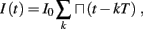
where ⊓(x) is the pulse shape, of width t₀ ≪ T (so ⊓(x) = 0 for x outside [0, t₀]), and unit magnitude, with I₀ being the current amplitude of the pulses (Figure 1). In numerical simulations¹ we used first order Euler integration (or Euler-Maruyama for stochastic simulations) with a time step of dt = 5 μs (quantitative results were verified also at dt = 0.5 μs). Each stimulation pulse was given as a square pulse with a width of t₀ = 0.5 ms and amplitude I₀. The results are not affected qualitatively by our choice of a square pulse shape. In the following discussion, we analyze the neuronal input/output (I/O) relation quantitatively with respect to f_in but only qualitatively with respect to I₀. Since the amplitude dependence is of secondary importance here we do not write explicitly any dependence of the parameters on I₀.

FIGURE 1

Figure 1. Schematic representation of the stimulation and the measured response. No APs are spontaneously generated. When stimulating a neuron with a periodic current pulse train with period T and amplitude I₀ we get either an AP-response or no-AP-response after each stimulation. In the former case an AP appears with a latency L, where L ≪ T. Inset: AP voltage trace. An AP is said to occur if V_th was crossed, and the AP latency L is defined as the time to AP peak since the stimulation pulse (more precisely, its beginning).

The two neuronal response features explored in Gal et al. (2010) are the occurrence of Action Potentials (APs) and their latency. Therefore, we too shall focus on these features. More precisely, we define an AP to have occurred if, after the stimulation pulse was given, the measured voltage has crossed some threshold V_th (we use V_th = −10 mV in all cases). The latency of the AP, L, is defined as the time that passed from the beginning of the stimulation pulse to the voltage peak of the AP (Figure 1, inset). Note that no APs are spontaneously generated.

2.1. Basic HH Model

Similarly to many discussions of neuronal excitability, we begin with the classical Hodgkin-Huxley (HH) conductance-based model (Hodgkin and Huxley, 1952):

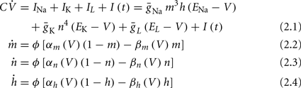
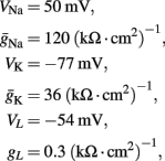
where I(t) is the input current, V is the membrane’s voltage and m, n, and h are the gating variables of the channels and the parameters are given their standard values (as in Hodgkin and Huxley, 1952; Ermentrout and Terman, 2010):

C_m = 1 μF/cm², Φ = 1, and we used the standard kinetic rate functions

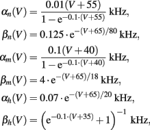
where in all the rate functions V is used in millivolts units.

We first note a discrepancy between this model and the experiment – the width of the AP in the model is twice as large in the model than in the experiment. To compensate for this we set the temperature factor Φ = 2 and the capacity C_m = 0.5 μF/cm², increasing the speed of the HH model dynamics by a factor of two, which results in the correct pulse shape (Figure 2, inset). We refer to the model with these fitted parameters, as the “fitted HH model,” while the model with the original parameters will be referred to as the “original HH model.”

FIGURE 2

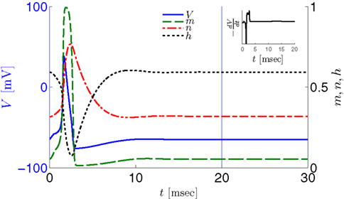
Figure 2. Fitted HH model variables V, m, n, and h after an AP relax to steady state on a shorter timescale than the minimal stimulation period used (T ≥ 20 ms for Gal et al., 2010, marked as a vertical line). This remains true when no AP is generated, since then the perturbation from steady state is even smaller. This timescale separation indicates that the system has no memory of previous pulses – so all stimulation pulses produce the same response. Note also that the AP voltage pulse width is similar to Figure S1B of Gal et al. (2010). Inset: −dV/dt during an AP, which is proportional to extracellular measured voltage trace (Henze et al., 2011). The AP pulse width is similar to Figures 1B, 2A, and 5C of Gal et al. (2010). Parameters: I₀ = 15 μA.

However, in either case, the HH model alone cannot reproduce the results in Gal et al. (2010). In both versions of the HH model, given a short pulse stimulation generating an AP, all the HH variables (V, m, n, and h) relax to close to their original values within ∼20 ms (Figure 2). Therefore, pulse stimulation at frequency f_in < 50 Hz (or T > 20 ms), as in the experiment, would result in each stimulation pulse producing exactly the same AP each time. This “memory-less” response is far too simple to account for complex behavior seen in the experiment, and so the model must be extended. In the next section we discuss how this is generally done.

2.2. HH Model Deterministic Extensions

The HH model has been extended many times since its original development (Hodgkin and Huxley, 1952), in order to account for the morphology of the neuron and for additional ionic currents as well as other processes that had been discovered (Hille, 2001; Bean, 2007). These extensions are generally done in a similar way, by adding more variables that represent either different neuronal compartments or various cellular processes, such as accumulating changes in the cell’s ionic concentrations or slow inactivation of ion channels (see Izhikevich, 2007; De Schutter, 2010; Ermentrout and Terman, 2010 for a modeling-oriented review of this subject). Such models were used, for example, to explore neuronal adaptation and bursting activity (e.g., Marom and Abbott, 1994; Fleidervish et al., 1996; Powers et al., 1999; Pospischil et al., 2008). The general form of such a conductance-based neuron model must include some spike-generating mechanism with rapid variables r ≜ (r₁, …, r_m)^⊤ ((·)^⊤ denotes transpose), along with slow variables s ≜ (s₁, …, s_n)^⊤, modulating the spikes over time:

where ∊ > 0 is some small parameter – rendering the dynamics of s (of timescale τ_s) much slower than the dynamics of r (of timescale τ_r). We shall assume for simplicity that all slow variables are normalized to the range [0, 1] (as is usually done for gating variables).

For example, the HH model is a special case of this model where r = (V, m, n, h)^⊤, equation (2.5) are given by equation (2.1–2.4) and all other quantities are held fixed, so ∊ = 0. Other basic models of excitable neurons also exist (Fitzhugh, 1961; Morris and Lecar, 1981). In any case, we require that, given a constant value of s (if ∊ = 0), the rapid variables r and equation (2.5) represent an “excitable,” non-oscillating, neuron. By that we mean that:

1. r remains at a unique constant steady state if I(t) = 0 (“resting state”).

2. After each stimulation pulse, for certain values of initial conditions and I₀, we get either a stereotypical “strong” response (“AP-response”) or a stereotypical “weak” response in r (“no-AP-response”). Only for a very small set of values of initial conditions and I₀, do we get an “intermediate” response (“weak AP-response”).

3. All responses are brief, and r rapidly relaxes back to steady state, within time τ_r. For example, τ_r < 20 ms in both versions of the HH model (Figure 2).

Next assume that ∊ > 0. Now s are allowed to change, and to modulate the neuronal activity in a history dependent way. Recall that the dynamics of s are slow since ∊ is small, and therefore ∊⁻¹ ∼ τ_s ≫ τ_r. For simplicity, we assume, as is commonly done (Izhikevich, 2007; Ermentrout and Terman, 2010), that h_i(r, s) = h_i(r, s_i), a linear function,

where δ_i and γ_i are kinetic rate functions of magnitude ∊. Some of this paper’s main results can be extended to general monotonic functions h_i(r, s_i) (see section C). Next we discuss some of the specific models we use in this work. Since we are interested in the temporal rather than the spatial structure of the neuronal response, we shall concentrate on single compartment (isopotential) models which include additional slow kinetic processes.

2.2.1. HHS model: basic HH + sodium slow inactivation

The work of De Col et al. (2008), which has some similarities with the work in Gal et al. (2010), implicates slow inactivation of sodium channels in the latency changes of the AP generated in response to stimulation pulses – as in the transient phase observed in Gal et al. (2010). Since slow inactivation of sodium channels (Chandler and Meves, 1970) has also been implicated in spike-frequency adaptation (Fleidervish et al., 1996; Powers et al., 1999 and in axonal AP failures Grossman et al., 1979a), and since in Gal et al. (2010) the latency change is clearly coupled with the spike failures (e.g., the existence of a critical frequency), we first wanted to examine whether slow inactivation of sodium channels alone can explain the experimental results. We incorporate this mechanism into the HH model (as in Chandler and Meves, 1970; Rudy, 1978; Fleidervish et al., 1996), by introducing s, a new slow inactivation gate variable, into the sodium current

We model s as having first order kinetics,

with voltage-dependent inactivation rate γ(V) = 3.4·(e^{−0.1·(V+17)}+ 1)⁻¹ Hz and recovery rate δ(V) = e^−(V+85)/30 Hz as in Fleidervish et al., 1996; again, in all the rate functions V is used in millivolts units). We call this the “HHS model.” In order to make the timescale of the transient change in the latency comparable to that measured in Gal et al. (2010), Figure 4A, we had to make the rates γ and δ 20 times smaller (such small rates were previously demonstrated (e.g., Toib et al., 1998). Also, using the fitted HH model, which had a narrow AP, required us to increase the inactivation rate γ to three times its original value, so sufficient inactivation could occur. However, this last change made inactivation level at rest too high, so we compensated by increasing the steepness of the activation curve of γ to three times its original value. The end result of this was γ(V) = 0.51·(e^{−0.3·(V+17)} + 1)⁻¹ Hz and δ(V) = 0.05e^−(V+85)/30 Hz. Using these rates together with the fitted HH model, we get the “fitted HHS model,” which reproduces the experimentally measured timescales of the transient response (Figure 8A). Alternatively, if instead we refer to the “original HHS model,” then it is to be understood that we used the original parameters of the HH model and γ(V) and δ(V), as in Fleidervish et al. (1996). Finally, we comment that sodium channels’ recovery from slow inactivation is known to be history dependent and to occur at multiple timescales (Toib et al., 1998; Ellerkmann et al., 2001). And so, one could argue that simple first order kinetics as in equation (2.8) are not accurate enough to describe the channel’s behavior. However, in neurons under pulse stimulation, the linear form of equation (2.8) is actually quite general – since Soudry and Meir (2010) showed how in this case equation (2.8) approximates the dynamics of an ion channel with power law memory which reproduce the results of Toib et al. (1998), Ellerkmann et al. (2001). Therefore, the response of the HHS model with slow inactivation of sodium as described in Soudry and Meir (2010) is not significantly different from the response using equation (2.8).

2.2.2. HHSAP model: HHS model + potassium activation

Slow activation of potassium current (either voltage or calcium dependent) has been implicated many times in reducing the neuronal excitability after long current step stimulation, termed “spike-frequency adaptation” (e.g., Koch and Segev, 1989; Marom and Abbott, 1994; Pospischil et al., 2008). When we take this into consideration we change the fitted HHS model, rename {s, γ, δ} → {s₁, γ₁, δ₁}, and add a slowly Activating Potassium current with M-current kinetics similar to those of Koch and Segev, 1989, Chapter 4), so the total potassium current is

with and

where

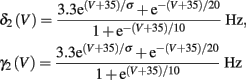
In Koch and Segev (1989), σ = 40 mV, while we used σ = 15 mV (again, in all the rate functions V is used in millivolts units). We refer this model as the “HHSAP model.”

2.2.3. HHSIP model: HHS model + potassium inactivation

Both slow inactivation of sodium channels, and slow activation of potassium channels have similar affect on the neuronal excitability – they act to reduce it after an AP. As we shall see later, this “negative feedback” type of behavior always results in very similar neuronal dynamics. However, “positive feedback” type of behavior is also observed – increased excitability after a depolarization (Hoshi and Zagotta, 1991). To account for this we take the HHSAP model, and switch the potassium rates {γ₂, δ₂} → {δ₂, γ₂} – so now potassium is Inactivating (“positive feedback”) instead of Activating (“negative feedback”). We name this the “HHSIP model.”

2.3. Simplifying Deterministic Conductance-Based Models

Deterministic Conductance-Based Neuron Models (CBNMs) are usually explored numerically, with the exception of several dynamical systems reduction methods (Izhikevich, 2007; Ermentrout and Terman, 2010). However, since in this work we concentrate only on a specific form of stimulation (T-periodic, short current pulses with amplitude I₀) which fulfills a timescale separation assumption [equation (2.9)]

allows us to replace the full model with a simpler, approximate model. This condition is applicable here, since for all the specific models we use (both fitted and original HH, HHS, HHSAP, and HHSIP models, described in the previous sections), τ_r ∼ 10 ms and τ_s ∼ 10 s, and since the stimulation protocol in the experiment, used the (physiologically relevant) period range of 20 ms < T < 1 s. Numerically, we found in all these specific models, that the analytical results stemming from this assumption remain accurate if f_in ≤ 30 Hz.

Since τ_r ≪ T (e.g., Figure 2) and since we deal with an excitable (non-oscillatory) neuron (as defined in 2.2), then after each stimulation pulse, whether or not there was an AP, the rapid variables relax to a unique steady state and do not directly affect the neuronal response when the next stimulation is given. Only s, a vector representing the slow variables of the system [equation (2.6)], retains memory of past stimulations. Therefore, to determine the neuronal behavior, it is only necessary to consider the dynamics of s and how it affects the system’s response. Thus, we consider how the neuronal response is determined by s.

2.3.1. Firing threshold

In response to a stimulation pulse with amplitude I₀ an AP will occur if and only if the “excitability” of the neuron is high enough. Since only s retains memory of past stimulations, we should only care about the dependence of this excitability in the value of s, so we write it as a function E(s) – where we say that an AP will occur if and only if E(s) > 0. We denote by Θ the threshold region – a set of values in which each s fulfills E(s) = 0. We calculated numerically the location of this threshold region from the full conductance-based model [equations (2.5 and 2.6)]. First, we set ∊ = 0, disabling all the slow kinetics in the model. Then, for every value of s we simulated this “half-frozen” model numerically by first allowing r to relax to a steady state and then giving a stimulation pulse with amplitude I₀. If an AP was generated then E(s) > 0, and E(s) ≤ 0 otherwise.

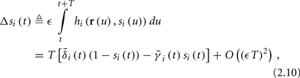
For example, in the context of the HHS model, the sodium current is depolarizing. Therefore, the stronger the sodium current, the more likely it is that an AP will be generated after a stimulation pulse. Since the sodium current increases with s, then if and only if s is above a certain threshold, which we denote by θ, the sodium current will be strong enough to create an AP. So, in the HHS model (or anytime s = s, a scalar) we can always write E(s) = s − θ (Figure 3A). In the HHSAP and HHSIP models (for which s = (s₁, s₂)) we found numerically that the shape of Θ is linear (see Figure 3B), so we can write E(s) = w·s − θ. Generally, we expect E(s) to be monotonic in each component of s separately, and monotonically increasing in I₀. Therefore, in the HHS model, we expect the threshold θ to decrease with I₀ (Figure 3A).

FIGURE 3

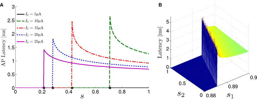
Figure 3. AP threshold and latency. (A) AP latency, L(s), calculated numerically from the fitted HHS model by setting ∊ = 0, and simulating the neuronal response at different values of s and I₀. Firing thresholds θ ≜ {s|E(s) = 0} are marked by black circles for each I₀. When no AP occurred, we define L ≜ 0. (B) Similarly, we calculated AP latency in the HHSAP and HHSIP models for I₀ = 8 μA. Notice the linear shape of the threshold line Θ.

2.3.2. Latency function

When an AP occurs in response to a stimulation pulse, its different characteristics (amplitude, latency, etc.) are also determined by s. We are interested mainly in the latency of the AP, and so we define the latency function L = L(s) for all s for which an AP occurs (when E(s) > 0). This function was also found numerically. For every value of s we simulated the “half-frozen” model (with ∊ = 0) response to a stimulation pulse, and measured the latency of the resulting action potential (when it occurred). For example, in the context of the HHS model, as can be seen in Figure 3A, an AP will have a smaller latency (faster membrane depolarization) the higher are s and I₀ – since both the sodium current and the stimulation current are depolarizing. See Figure 3B for the (2D) latency function in the HHSAP and HHSIP models.

2.3.3. Dynamics of s

Having described how s affects the neuronal response, all that remains is to understand how s evolves with time.

Using equations (2.6 and 2.7) we write

where we have used the following notation for a time-averaged quantity

We neglect the O((∊T)²) correction term, since ∊T ≪ 1. Since the value of s(t) determines the r dynamics in the interval [t, t + T], it also determines and . Thus, slightly abusing notation, we write _i(s(t)) and instead of and δ_i(t), respectively. Since the condition determines whether or not an AP is generated, we expect that generally the sharpest changes in the values of and occur near the threshold area Θ where E(s) = 0. Following this reasoning, we make the assumption that the kinetic rates may be approximated as step functions with discontinuity near E(s) = 0,

The interpretation of this assumption is that the kinetic rates are insensitive to the s induced changes the AP shape and the steady state of r. For example, in the context of the HHS model, as can be seen in Figure 4B, we get for the rate of sodium inactivation

where γ₊ > γ₋, while the recovery rate remains constant

FIGURE 4

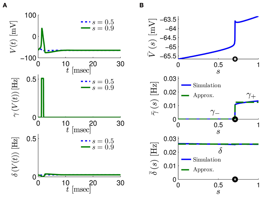
Figure 4. Calculation of the average kinetic rates in the fitted HHS model, where s is held constant. (A) Dynamics of voltage V(t) (top) γ(V(t)) (middle) and δ(V(t)) (bottom) after a stimulation pulse, plotted for two values of s. For s = 0.5 no AP occurred, while for s = 0.9 an AP was generated. Notice how γ(V(t)) increases dramatically during an AP, while δ(V(t)) does not. (B) We derived (top) (middle) and (bottom) using equation (2.11), by simulations as in (A), for many values of s. Firing threshold θ is marked by a black circle. Notice that changes significantly more than especially near θ, and that we can approximate to be a γ_±-valued step function as in equation (2.12) while a constant. I₀ = 10 μA, T = 50 ms with V, m, n, h initial conditions set at steady state values (which can be somewhat different for each value of s).

As can be seen in Figure 5, for the HHSAP model, we get

with and In the HHSIP model, and are switched.

FIGURE 5

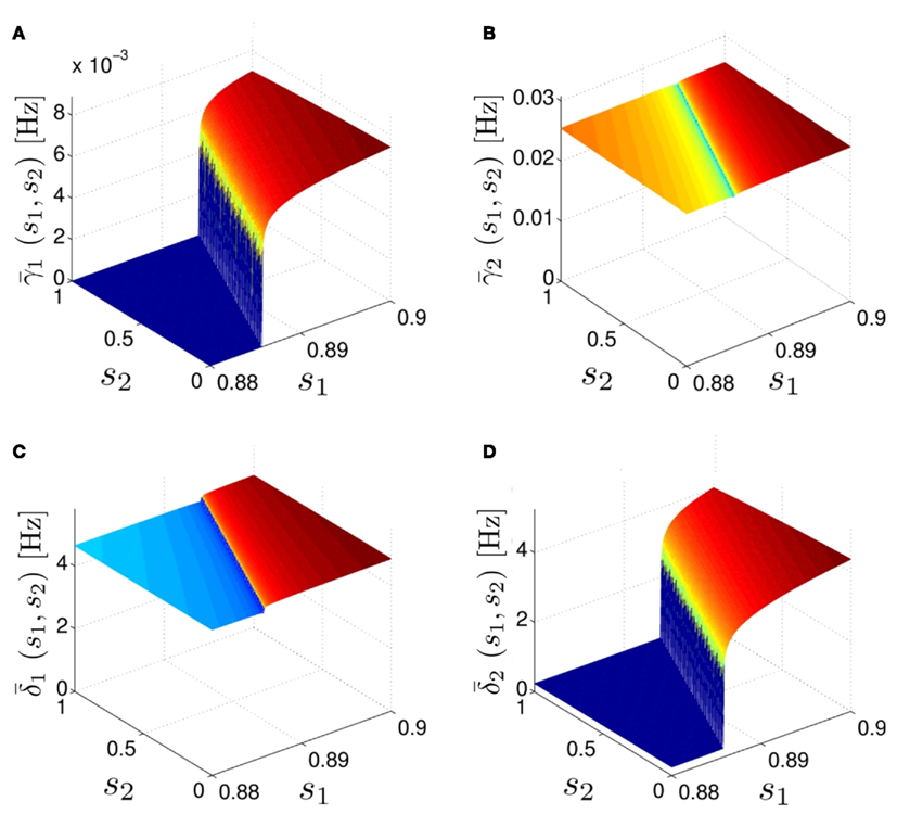
Figure 5. Average activation and inactivation rates for the HHSAP model, where s is held constant. (A) (B) (C) (D) and are almost constant, while and have a sharp discontinuity near the threshold area Θ (Figure 3B). I₀ = 8 μA, T = 50 ms with V, m, n, h initial conditions set at steady state value.

In conclusion, together with equations (2.10 and 2.12) gives

which is a diagonal, piecewise linear (or, more accurately, affine) recursive map for s. Similar discontinuous maps appear in many systems (Di Bernardo, 2008), and recently also in neuroscience (Ibarz et al., 2011). However, in contrast to this recent work, our method of discretization relies on the stimulus pulses arrival times, thereby allowing greater analytical tractability in our case.

2.3.4. Dependence of kinetic rates on stimulation

Next, we show that and are all linear in f_in. Expressing the integral on [t, t + T] in equation (2.11) as the sum of two integrals on [t, t + τ _r ] and [t + τ_r, t + T], we exploit the fact that most of the response in r(t) after an AP is confined to [t, t + τ_r] (since τ_r ≪ T; Figure 4A). Denoting

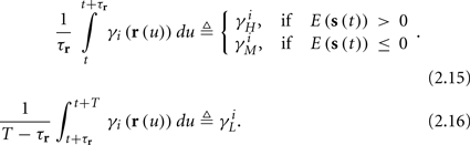
and using γ_H, γ_M, γ_L (which are independent of T) we get from equations (2.11 and 2.12)

Similarly defining we obtain

Notice that since τ_r f_in is small (since τ_r ≪ T), can be significantly different from if and only if and so, necessarily, Additionally, since γⁱ(r) are usually monotonic functions, we get If instead then we do not care much about anyway. This reasoning applies also to the recovery rates , to the HHS model, where we get that (implied also from Figure 4A), and also in the HHSAP and HHSIP models.

Finally, we note that since I₀ has little effect on the steady state of r (e.g., rest voltage), and just a mild effect on the development of r during an AP (“all-or-none response”), are expected to have a very small dependence on I₀. Simulations confirm this low sensitivity to I₀ for and for the specific models we considered, so hereafter we assume they are all independent of I₀ for the specific models used. However, we may see an increased sensitivity of and to I₀ if I₀ is increased, or the voltage threshold of the corresponding kinetic rate (V_1/2) is decreased.

2.4. Simplified Deterministic Model Analysis

To summarize the main results of section 2.3, any extension to the HH model of the generic form [equations (2.5–2.7)] can be greatly simplified under pulse stimulation given the following two assumptions:

1. Timescale separation [equation (2.9); Figure 2]

2. Step-like behavior of the average kinetic rates [equation (2.12); Figures 4 and 5].

In this case we can write a simplified model for the dynamics of s = (s₁,…, s_n)^⊤ and the neuronal response:

1. At each stimulation an AP is produced if and only if E(s) > 0, where E(s) is “the excitability function,” calculated numerically (Figure 3).

2. The latency of an AP is also determined by a function – L(s), calculated numerically (Figure 3).

3. The change in s between consecutive stimulations is given by the piecewise linear map in equation (2.14).

4. The inactivation and recovery rates and all change linearly with f_in, as derived in equations (2.18 and 2.19).

Additionally we note that for the specific models we examined as I₀ increases, E(s) increases, L(s) decreases, while all the other parameters remain approximately constant (Figure 3). Although this behavior does not follow directly from the assumptions as do the above results, we expect it to remain valid in many cases (see section 2.3). This model is mainly useful in order to analyze and explain the dynamics of the full conductance-based model [equations (2.5–2.7)], as we do next. However, all numerical simulations are performed on the full conductance-based model, to demonstrate the validity of our results. In section B we further explain our assumptions, and in section C we show how we can replace some of the them with weaker assumptions.

2.4.1. Transients

In equation (2.14) each s_i is coupled to the others only through the threshold. Therefore, if s(0) is far from the threshold area E(s) = 0, each s_i will change independently forever, or until s(t) reaches the threshold area E(s) = 0. Until this happens it is perhaps more intuitive to describe the dynamics by the coarse-grained continuous-time version of equation (2.14),

The solution, for each case, is given by

where

is the timescale of the exponential relaxation, and

so s(t) relaxes toward depending on whether

2.4.2. Steady state

Eventually s(t) arrives at some stable steady state behavior. There are several different possible steady state modes, depending on which are affected by the amplitude and frequency of stimulation. These can be found by the following self-consistency arguments.

1. Stable: if then s(t) stabilizes at so APs are generated after each stimulation.

2. Unresponsive: if , then s(t) stabilizes at so no APs occur.

3. Bi-stable: if then, depending on the initial condition, s(t) stabilizes either on (as in the stable mode) or on (as in the unresponsive mode). This type of behavior is exhibited only in cases when the neuron becomes more excitable after an AP (“positive feedback”).

4. Intermittent: if then steady state is always “on the other side” of the threshold. Thus s(t) will stabilize near the threshold E(s) = 0. In this regime, small changes in s dominate the behavior of the neuron: the neuron alternates between an “on” state, in which E(s) > 0 and the neuron can generate an AP at each stimulation, and an “off” state in which E(s) ≤ 0 and the neuron does not generate any AP. This type of behavior is exhibited in cases when the neuron becomes less excitable after an AP (“negative feedback”).}

2.4.3. Firing rate

Suppose we count the number of AP generated over m stimulation periods in steady state, and denote by the time-averaged probability of generating an AP. Assuming that the system has indeed arrived to a steady state, for large enough m, p_m does not depend on m, so we denote it just by p. The only case where p ≠ {0, 1} is the intermittent mode. At this mode s is near the threshold E(s) = 0, so p can be derived by solving the self-consistent equation

where we defined and Also, notice that if, for all i, and then we can rewrite equation (2.24) in the form h(pf_in) = 0, which entails that in this case

2.4.4. Firing patterns

Assume that equation (2.23) has been solved for p. Under the assumption that in steady state s remains near s_∞ (p), from equations (2.12 and 2.14) we get that if E(s) > 0 and if E(s) ≤ 0, where

Simple algebra gives that for all i, This means that Δs⁺ has the opposite direction to Δs⁻ – so s remains on a simple one-dimensional limit cycle. If 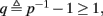the AP firing pattern is simple and repetitive: one period with an AP, followed by either ⌊q⌋ (integer part of q) or ⌊q⌋ + 1 periods in which no AP occurred (Figures 6A,C). If instead q < 1, the firing pattern is different, yet still simple and repetitive: one period in which no AP occurred, followed by either ⌊q⁻¹⌋ or ⌊q⁻¹⌋ + 1 periods with APs (Figure 6B). These two simple firing patterns are the only possibilities in the 1D case (s = s). However, in some other cases, this simple description cannot be true, as we explain next. Assume that s remains near s_∞(p). In this case we can linearize where . Without loss of generality, assume that q > 1 and 0 < w^⊤ (s − s_∞ (p)) at a certain period, so an AP is produced. In this case, according to the above description, s increases in the next period to s + Δs⁺, and no AP is produced – so 0 ≥ w^⊤ (s − s_∞ (p) + Δs⁺). But this necessarily means that 0 > w^⊤Δs⁺. If this condition is not fulfilled (or, equivalently, 0 < w^⊤Δs⁻), then the above description of the firing patterns cannot be correct. Instead, s will still revolve around s_∞(p), but now in a higher-dimensional limit cycle (not 1D). In this case, the firing patterns are somewhat more general than before: s may remain on one side of the threshold Θ for several cycles, so the neuron can fire a continuous AP-response sequence for L₊ periods, and then remain silent (no-AP-response sequence) for L₋ periods, where both L₊ > 1 and L₋ > 1 (Figure 6D). We noticed numerically that even in this case, the value of q still approximates the L₊/L₋ ratio (Figure 9D).

FIGURE 6

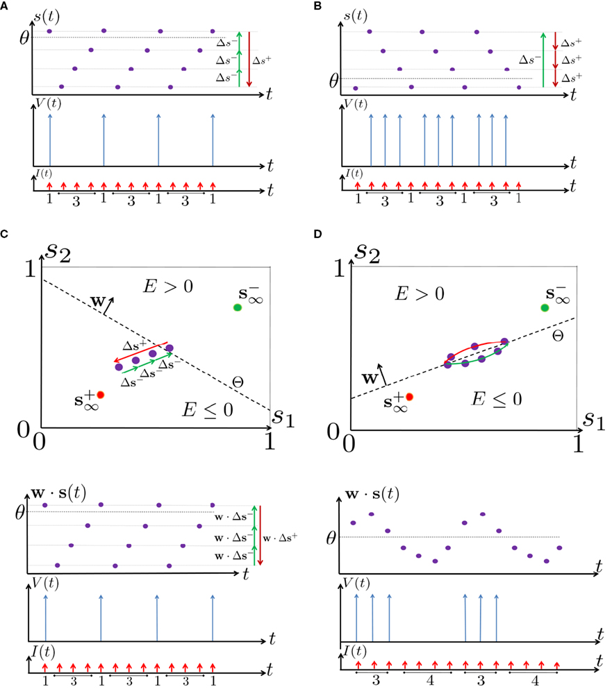
Figure 6. Schematic state space dynamics of s and firing patterns in the intermittent mode. Recall that 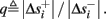The simple dynamics of the 1D model are shown with (A) q = 3 and (B) q = 1/3. For the 2D model, the dynamics can be slightly more complicated. (C) For w^⊤Δs⁺ < 0 we get, from equation (2.25), a 1D limit cycle with Δs⁺ = − qΔs⁻ (top, with q = 3). This results in a 1: q (AP:No AP) firing pattern (bottom). (D) For w^⊤Δs⁺ > 0 we obtain a 2D limit cycle (top) which results in m:n firing patterns (“bursts”; bottom). See Figures 9A–C for the corresponding numerical results.

In addition to the above approximate analysis, there are several general attributes of the steady state solutions of equation (2.14), that lead us to believe that the firing patterns do not generally exhibit complex patterns. These attributes are the following:

• Finite, periodic: in the 1D case, as was explained above, the firing patterns are periodical and composed of only two basic repeating sub-patterns, but the overall period of a firing pattern may be arbitrarily long. However, as the duration of the overall period increases, the relevant parameter space (that can produce such a period) decreases (Tramontana et al., 2010) – so an infinitely long period can be achieved only in an (uncountable) parameter set of measure zero (Keener, 1980). A similar result is expected to hold in higher-dimensional systems, since, as in the 1D case, infinitely long periods seem to be generated only in the rare (measure zero) cases (bifurcations) in which the steady state (finite) limit cycle touches the threshold.

• Stable, non-chaotic: since equation (2.14) is a piecewise linear diagonal contracting map (namely, |d(s_i + Δs_i)/ds_i| < 1), its eigenvalues are inside the unit circle, so any finite limit cycle that does not touch Θ must be stable (Thompson and Stewart, 2002, or section A.1). It can be shown that this remains true even when h_i (r, s_i) [equation (2.7)] is not linear (but still monotonic), or when the timescale separation assumption τ_r ≪ T ≪ τ _s is relaxed to τ _r ≪ min (T, τ _s ) (section C).

• Globally stable, unique: in the 1D case it was further proved (Keener, 1980, or section A.2) that any such limit cycle must also be globally stable – and therefore unique. Numerical simulations indicate that such global stability (or, uniqueness) remains true in higher-dimensional systems. However, a direct proof of this might be hard, due to results of Blondel et al. (1999).

• Bounded L_± durations: in the intermittent mode (where ), from equation (2.21), we get 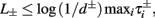where 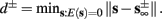And so, the lengths of the L_± periods are bounded if and d^± ≠ 0. Again, the latter condition is violated only for a measure zero set of parameters.

We emphasize that if even any of the above mentioned exceptions are reached (either a limit cycle or touching Θ) – these rare cases will be structurally unstable, meaning they will disappear if infinitesimally small changes occur in almost any parameter, such as stimulation rate or amplitude.

3. Results

In Gal et al. (2010), a single synaptically isolated neuron, residing in a culture of rat cortical neurons, is stimulated with a train of extracellular periodic current pulses. This neuron is isolated from other neurons by blocking all synaptic activity in the network. For sufficiently strong pulse amplitudes the neuron sometimes responds with a detectable AP. The observed neuronal response was characterized by three different modes (Gal et al., 2010; Figure 2). When the neuron is stimulated at low frequencies (e.g., 1 Hz) it always responds reliably with an AP, which peaks after the stimulus with a constant latency (∼5 ms). This mode is termed a “stable mode.” When the neuron is stimulated at higher frequencies, it begins to adapt and the latency of its APs increases. This phase is termed “transient mode.” If the stimulation frequency is higher than a certain “critical frequency” (2–23 Hz) the transient mode terminates when the latency reaches a certain “critical latency” (∼10 ms). When this critical latency is reached, the neuron enters a phase in which it sometimes “misses,” and an AP is not created in response to the stimulation pulse. When an AP is created, its latency fluctuates around the critical latency. This kind of irregular mode is termed the “intermittent mode.” When the frequency of stimulation is changed back to low frequencies (e.g., 1 Hz) the behavior switches back again to a transient phase, in which the latency now decreases back to its original steady state value in the stable mode.

The main additional observations of Gal et al. (2010) can be summarized as follows:

1. The critical latency of the intermittent mode does not depend on the stimulation frequency (Gal et al., 2010; Figures 4A,D).

2. The rate of change in latency during the transient mode increases linearly with stimulation frequency (Gal et al., 2010; Figure 4B).

3. The firing rate in the intermittent mode decreases moderately with stimulation rate (Gal et al., 2010; Figure 4C).

4. The response of the neuron in the stable and transient mode is almost exactly repeatable (Gal et al., 2010; Figure 9).

5. During the intermittent mode, regular “burst”-like firing patterns appear (Gal et al., 2010; Figure 8D).

6. During the intermittent mode, irregular firing patterns appear (e.g., Gal et al., 2010; Figures 8C,E,F).

7. The irregular patterns of response in the intermittent phase are not repeatable (Gal et al., 2010; Figure 9).

8. The variability of the AP latency fluctuations increase with the latency magnitude during the transients (Gal et al., 2010; Figures 4A,D), and reaches a maximum in the intermittent mode.

9. During long recordings (55 h in Gal et al., 2010; Figures 5A,B,D) it was observed that the firing rate, and the type of firing patterns (see also Gal et al., 2010; Figure 10), change with time. The shape of the AP, however, remains stable throughout the experiment (Gal et al., 2010; Figure 5C).

10. The changes in the firing rate display self-similarity properties (Gal et al., 2010; Figure 6). This remains true for Poisson stimulation (Gal et al., 2010; Figure 7).

Our aim in this section is to find the minimal model capable of reproducing these results. In section 2.1 we have already established that for the classical HH model the response to each stimulation pulse must be the same and therefore cannot reproduce these results. Therefore, we begin by investigating the dynamics of the next simplest model – the HHS model (section 2.2.1), which includes also slow inactivation of sodium channels. As we show in section 3.1, the HHS model reproduces a significant portion of the experimental results (the different modes and observations 1–4), and its dynamics is easily explained using our simplified version (section 2.3).

However, the HHS model fails to generate the specific firing patterns seen in the experiment. In section 3.2 we extend the HHS model to the HHSIP model, enabling us to reproduce some of the burst patterns (observation 5). However, the irregular firing patterns (observation 6) raise a more serious obstacle, which cannot by easily surpassed by simply extending the model, taking into account additional variables representing the states of other types of channels or ion concentrations. We make the general argument (based on our analytic treatment) that the irregular patterns and variability (observation 6–10) cannot be created by such model extension, in the framework of a generic neuron model of the form of equations (2.5 and 2.6) and under our assumptions [equations (2.9 and 2.12)]. Taking this result into account we try to employ a different form of model extension. In section 3.3, we explore numerically the effects of ion channel noise on the results. We show that the sensitivity of the near-threshold dynamics of the neuron in the intermittent mode render such noise highly significant. Additionally, the stochastic model seems to better reproduce the variability of the experimental results in both the transient and intermittent modes. Finally, we reach the conclusion that extending from deterministic CBNMs to stochastic CBNMs is crucial if we wish to reproduce the details of the variability and the irregular patterns (observations 6–10). However, the analysis of a stochastic model requires different tools from those developed here. We therefore relegate the complete analysis of the stochastic model, and the reproduction of remaining results, to a companion paper.

3.1. HHS Model

As discussed in section 2.4, the full HHS model can be greatly simplified under pulse stimulation at low enough frequencies, as in Gal et al. (2010). Next, we explain how the different neuronal response modes seen in the experiment were reproduced, with the help of this simplification.

3.1.1. Transient mode

Assume an initial stimulation pulse had a current I₀ which was strong enough to generate an AP (as in Gal et al., 2010) – so we get the initial condition s(0) > θ on the sodium availability. According to equation (2.21) as long as s(t) > θ, s(t) decreases exponentially. Since the latency increases when s decreases this seems to confirm (Figure 7) to the experimentally observed transient mode (Gal et al., 2010; Figure 2). Additionally, according to the simplified model [equations (2.22 and 2.18)], the rate of the transient is indeed linear in the frequency of stimulation

as in Gal et al. (2010, Figures 4A,B). And indeed, using the fitted HHS model, we were able to numerically reproduce these results in Figure 8A. As can be seen there, the transient mode ends either in a stable steady state (when f_in is low), or in an intermittent mode, which occurs when s(t) reaches θ (Figure 8B), or equivalently, when the latency reaches L(θ) (Figure 8A) – the critical latency observed in the experiment. Also, as can be seen in Figure A1A, the duration of the transient mode also decreases when stimulation current I₀ is increased – since the threshold θ decreases with I₀ (Figure A1B). Note also that in all cases the latency of the AP is shorter and less variable than the measured one (Figure 8A). Later we address these discrepancies (in sections 4.4 and 3.3, respectively). Finally, we note that if, instead of the fitted HHS, we used the original HHS, the duration of the transient mode would be considerably shorter (∼1 s) – which indicates that perhaps the kinetic variable responsible for this slow transients is significantly slower than the slow sodium inactivation kinetics in Fleidervish et al. (1996).

FIGURE 7

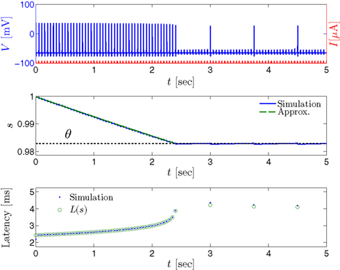
Figure 7. Fitted HHS model – transient mode and arrival to intermittent mode. Stimulation current pulses generate APs (top). Initially we are at the transient mode where APs are reliably generated each period until we reach intermittent mode, and AP failures start to occur. This happens since (middle) sodium channels availability s(t) decreases during the transient mode, due to slow inactivation caused by APs, until the excitability threshold θ is reached, and then s(t) starts to switch back-and-forth across θ (intermittent mode). Notice that analytical approximation of equation (2.21) closely follows the numerical result during the transient phase. Latency during transient mode (bottom) is increased, as in (Gal et al., 2010) Figure 2. Notice that, as expected, using the latency function L(s) (calculated numerically in Figure 3A) on s yields a similar value as the latency calculated by direct numerical simulation. I₀ = 7 μA.

FIGURE 8

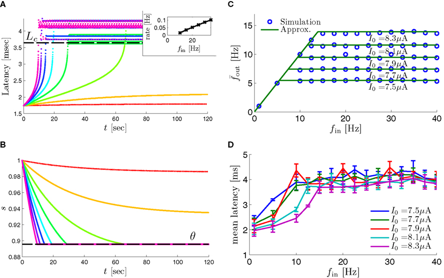
Figure 8. Fitted HHS model – response dependency on f_in. (A) Spike latency as a function of time from stimulation onset (each color designates a different stimulation rate): stimulation at I₀ = 7.9 μA and rates of f_in = 1, 5, 10, 15, 20, 25, 30, 35, 40 Hz (red, orange…,); The transient phase speeds up when f_in is increased, and ends at the same critical latency L_c. Similar to Figure 4A of Gal et al. (2010). Inset: the rate is the reciprocal of the timescale of the transient phase, defined as halftime the latency reaches the critical latency, as in Gal et al. (2010). Notice that the rate is linear in f_in, as predicted by equation (3.1), and similar to Figure 4B of Gal et al. (2010). Both of these results can be explained by (B) the sodium availability trace, s(t) [using same color code as in (A)] where s transient speeds up when f_in is increased, while θ does not change. (C) Dependency of steady state firing rate on stimulation frequency. Comparison between simulation and approximation of equation (3.3), for different values of I₀: in fitted HHS model – for (stable mode), and then for (intermittent mode). Compare with Figure 4C of Gal et al. (2010). Notice also that in both cases, increases with I₀, as expected from equation (3.2), and the fact that θ decreases in I₀. (D) Mean latency at steady state as a function of f_in, shows an initial increase [stable mode, where should indeed increase in f_in, by equations (2.23 and 2.18)] and then saturates (intermittent mode, where L ≈ L(θ) is indeed independent of f_in), as seen in (Gal et al., 2010) Figure 4D. Also, the error bars indicate the SD of the latency – or the latency fluctuations. These fluctuations increase in the intermittent mode, as seen in (Gal et al., 2010) Figure 4D, due to the back-and-forth motion of s around θ at this mode, and the high sensitivity of L(s) near s = θ.

3.1.2. Steady state

In any case, eventually the transient mode ends, and s(t) arrives at some steady state behavior. Using the results of section 2.4, we first explore analytically all the different types of behaviors feasible in the context of the HHS model. The type of mode that would actually occur depends on the model parameters and the inputs f_in and I₀. Using equations (2.18, 2.23, and 2.24) we find that there are three different possible steady states, depending on the two parameters and given by

Note that corresponds to the measured critical frequency, while larger than is a second critical frequency, which was not observed in Gal et al. (2010). Note that increases with I₀, since θ decreases with I₀ (Figure 8C). Specifically, increases quadratically with I₀ (Figure A1C), similarly to θ⁻¹ (not shown).

If then and s(t) stabilizes at namely above the threshold θ, implying that each stimulation generates an AP (as the steady state for f_in = 1.5 Hz in Figure 8A). The latency of the AP in this case is stable at (Figure 8D). Therefore, this mode seems to agree with the experimentally measured stable mode in Gal et al. (2010).

If then and s(t) stabilizes on namely below the threshold θ, and no APs are fired. We refer to this as the “unresponsive mode,” which was not reached in the experiment. It is possible that if a higher f_in or I₀ were used, then such a mode would be achievable. However, it is also generally possible that violates the timescale separation assumption τ_r ≪ T, so that this mode could be unattainable at the specific parameter values used. In the context of the fitted HHS model this violation indeed occurs and also is much higher than any physiological stimulation rate. However, if other parameters were used (e.g., larger γ_M) then such a mode could be attainable at relevant frequencies.

If then so the steady state is always “on the other side” of the threshold. Therefore, s(t) will always return to θ – whether above or below. Thus, in this case, the threshold has become effectively the new steady state of s(t) (Figure 7, middle). In this regime, small changes in s dominate the behavior of the neuron: the neuron alternates between an “on” state, in which s(t) > θ, where it generates an AP after each stimulation, and an “off” state in which s(t) ≤ θ, where it does not generate any AP. This steady state is reached when s hits the threshold θ, or, equivalently, when the latency reaches a critical latency ≈L(θ). Due to the back-and-forth motion of s around θ at this steady state, and the high sensitivity of L(s) near s = θ (Figure 9A), we get much larger fluctuations in the latency than in the stable mode (Figure 8D). Together, these properties render this type of steady state qualitatively similar to the experimentally measured intermittent mode in Gal et al. (2010).

FIGURE 9

Figure 9. Firing patterns and excitability dynamics in the intermittent mode, for different models: (A) Fitted HHS. (B) HHSAP. (C) HHSIP. (D) Stochastic HHS (N = 10⁶). Blue circles – APs (1 – AP generated, 0 – AP failure), red – excitability function E(s) (s in HHS), green line – excitability threshold E(s) = 0 (θ in HHS). Notice that in deterministic models (A–C) APs occur if and only if E(s) > 0, and that the resulting firing patterns are regular, periodic, and depend very simply on q (calculated from model parameters). Specifically, in (A,B), when q ≥ 1 each AP must be followed by either ⌊q⌋ or ⌊q⌋ + 1 periods in which no AP occurred, and when q < 1 each AP failure must be followed by either ⌊q⁻¹⌋ or ⌊q⁻¹⌋ + 1 APs. These rather specific patterns are generated by the “up and down” motion of s around the threshold (as in Figure 6A–C), due to negative feedback. In contrast, the HHSIP model can generate m:n “burst”-like patterns, due to the positive feedback of potassium inactivation. Notice that as before, q still well approximates the ratio of (AP:No AP) response sequences lengths in the HHSIP. In contrast to deterministic models, the stochastic HHS allows a large variety of irregular patterns. I₀ = 7.7 μA

3.1.3. Intermittent mode – firing rate

In the intermittent mode, solving equation (2.24) together with (2.23) and (2.18) gives the an approximate expression for the mean firing rate

where we defined and the mean firing rate as where p is the time-averaged probability of generating an AP (defined in section 2.4). This linear equation approximates well the firing rate of the full HHS model as long as the timescale separation assumption [equation (2.9)] holds true. In the fitted HHS model, this approximation fits well with numerical results up to f_in = 40 Hz (Figure 8C). Notice also that in that case we have a a ≪ 1, and since γ_M ≪ γ_H. If the sub-threshold inactivation γ_M is larger, then a is also larger, as can be seen, for example, in the original HHS model (Figure A2A), where γ_M is not negligible in comparison with γ_H. In any case equation (3.3) gives a decreasing linear I/O relation, which, combined with the simple relation in stable mode, gives a non-monotonic response function. This response function is similar to the experimental results (Gal et al., 2010; Figure 4C).

3.1.4. Intermittent mode – firing patterns

So far, the HHS model seems to give a satisfactory explanation for many of the experimental results observed in Gal et al. (2010). However, there is an important caveat. If the stimulus frequency obeys the timescale separation assumption [equation (2.9)], the HHS model can produce only very simple patterns during intermittent mode (Figure 9A). As explained in section 2.4, in the intermittent mode, s changes in approximately constant increments, Δs^±, close to the threshold θ, defined in equation (2.24): inactivation step Δs⁺ < 0 if s > θ and recovery step Δs⁻ > 0 if s ≤ θ. Defining as the ratio between step sizes, and assuming that q ≥ 1, we get that in any firing pattern each AP must be followed by either ⌊q⌋ or ⌊q⌋ + 1 periods in which no AP occurred (“no-AP-response sequence”; Figure 6A). If instead q < 1, then each AP failure (a period in which no AP occurred) must be followed by either ⌊q⁻¹⌋ or ⌊q⁻¹⌋ + 1 periods with APs (“AP-response sequence”; Figure 6B). We note also the q is related to the mean firing rate by q = p⁻¹ − 1, and that in the fitted HHS model the step sizes around the threshold are very small which is an important fact we will use later (in section 3.3). In any case, as explained intuitively above, it can be formally proven that the firing patterns in the intermittent steady state are always regular, periodic, and globally stable – as also seen numerically in Figure 9A. Such firing patterns are not at all similar to the highly irregular firing patterns observed experimentally (e.g., Gal et al., 2010; Figure 8). Also, we clearly see in some of the experimental figures m:n “burst” patterns in which m > 1 APs are followed by n > 1 AP failures (e.g., Gal et al., 2010; Figures 8D,E) – which cannot be produced by the HHS model. Therefore, in the next section, we revise the model, in an effort to account for these discrepancies.

3.2. The Addition of Kinetic Variables

As we saw in previous section, the fitted HHS model can reproduce many experimental results. However, it has one major flaw – in the relevant stimulation range it can produce only very simple, regular, and periodic firing patterns in the intermittent mode – in contrast with the irregular firing patterns of Gal et al. (2010). How should the model be extended in order to reproduce this? Suppose we use a more general model for a point neuron [equations (2.5–2.7)]. This general model may include an arbitrary number of slow variables, each corresponding to some slowly changing factor that affects excitability – such as the availability of different types of channels or ionic concentrations. Can such a general model generate more complicated firing patterns? It seems trivial that a system that includes a wide variety of processes, at a large range of timescales, should be able to exhibit arbitrarily complex patterns, and even chaos. However, as explained in section 2.4, if this stimulus and the model adhere to our assumptions [namely, the timescale separation (equation (2.9)) and the step-like behavior of the average kinetic rates (equation (2.12)], this is not the case, chaos cannot occur, and again we conclude that only regular, periodic, and stable firing patterns are possible, except perhaps in a very narrow range of stimulus and model parameters (a “zero measure” set). This perhaps surprising result remains true for any arbitrarily complex conductance-based model (with arbitrarily large number of slow variables, and arbitrary slow timescales) as long as our assumptions remain valid.

What specific type of firing patterns are possible then, under these assumptions? If, for example, only “negative feedback” type slow variables exist (those which reduce excitability after an AP), such as potassium activation and sodium inactivation in the HHSAP model, then we get 1: n or n: 1 (AP: No AP) firing patterns as in the HHS model (Figures 6C and 9B). However, if sufficient “positive feedback” also exists (some slow variables contribute to a increased excitability after an AP), as potassium inactivation in the HHSIP model we can get a more general “burst” firing patterns of m:n (AP: No AP). However, these firing patterns are also expected to be very regular and periodic (Figures 6D and 9C). Such firing patterns were also observed experimentally (e.g., Gal et al., 2010; Figures 10B,C). The condition that separates both types of firing patterns’ dynamics depends on both parameters and stimulation. Therefore a neuron that has both positive and negative feedback can have “bursts” firing patterns in the intermittent mode, for a certain range of f_in and I₀. We note that the mechanism behind this burst firing pattern is similar in principle to the mechanism behind “slow wave” bursts, that can occur in the standard current step stimulation of neurons (Izhikevich, 2007).

And so, under our assumptions, the addition of more slow variables to the HHS model can only help to reproduce one additional response feature observed in the intermittent mode – namely, the “burst” firing patterns. The simplest extension that achieves this is the HHSIP model. Note also that in the HHSIP model we took the additional potassium current to be relatively weak (). Though this weak current can have a large impact in the intermittent mode (e.g., Figure 9C), it has a relatively small effect on the neural dynamics in the transient mode (Figure A3A). In most cases, this is desirable since the HHS model already fits nicely with experimental results in the transient mode, e.g., the existence of a critical latency and the simple linear timescale relation [equation (3.1)]. However, we should be careful not to destroy the fit of the HHS model during the transient phase if we extend it by adding additional slow kinetic variables. For example, by increasing we can generate an inflection point in the latency transients (Figure A3B), making them more similar to some experimental figures (e.g., Gal et al., 2010; Figure 2A) but less to others figures, which do not have an inflection point (e.g., Gal et al., 2010; Figure 4A). We may also want to increase the magnitude of the latency in the fitted HHS model, which is significantly smaller than that in Gal et al. (2010). As explained in section 4, this should be done by extending the model to include several neuronal compartments, through which the AP propagates and the latency accumulates. Such an extension is beyond the scope of this article.

3.3. Ion Channel Noise

Since deterministic CBNMs cannot reproduce the observed irregularity, we now examine the possibility that it could be produced by stochastic effects. Since synaptic activity was blocked in the experiment of Gal et al. (2010), the only other major source of noise is the stochastic ion channel dynamics (White et al., 2000; Hille, 2001; Faisal et al., 2008). The gating variables used in the conductance-based models to account for channel activation or inactivation (such as s in the HHS model) actually represent averages of a large number of discrete channels. Since the population of ion channels in the neuron is finite, the stochasticity in their dynamics is never completely averaged out, and can affect neuronal dynamics (Schneidman et al., 1998; White et al., 1998; Steinmetz et al., 2000; Carelli et al., 2005; Dorval and White, 2005), and, even more so, thin axons (Faisal and Laughlin, 2007) and dendrites (Diba et al., 2004; Cannon et al., 2010).

Consider the HHS model with channel noise added to it. A naive, yet common way to approximate this noise (Fox and Lu, 1994; Chow and White, 1996; Faisal, 2009, but see Goldwyn et al., 2011, Linaro et al., 2011) is to add a noise term to each of the gating variables representing the channels’ state. For example, equation (2.8) in the HHS model becomes a one-dimensional Langevin equation (Fox and Lu, 1994; Faisal, 2009)

where , N is the number of channels, and ξ is a Gaussian “white noise” process with zero mean and covariance cov [ξ(t), ξ(t′)] = δ(t − t′). Determining N, the physiologically relevant number of ion channels in the spike initiation area, still remains an open issue (e.g., Kole et al., 2008 vs. Fleidervish et al., 2010). Current crude estimates give N = 10⁴ − 10⁶ (Rowat, 2007). To demonstrate that stochasticity remains significant even at high channel numbers, we will use here N ≥ 10⁶. And indeed, a simulation of the stochastic HHS model (independent-subunit method, as described in Goldwyn et al. (2011) with N = 10⁶ yielded an irregular response in the intermittent mode, as observed in the experiment (Figure 9D). Moreover, the presence of noise (N = 10⁷) added latency fluctuations (Figure 10A) in the transient and intermittent modes rendering the model response more similar to the experimental results (Gal et al., 2010; Figure 4A), than in the deterministic case (Figure 8A) – specifically, notice the broadening of the latency variance during the transients. It is impossible to generate such latency fluctuations in the deterministic CBNMs (under our assumptions) since the transients in s are monotonic [and exponential, see equation (2.21)] – unless the latency function L(s) is non-monotonic and highly irregular (in contrast to the ones we found here – see Figure 3).

FIGURE 10

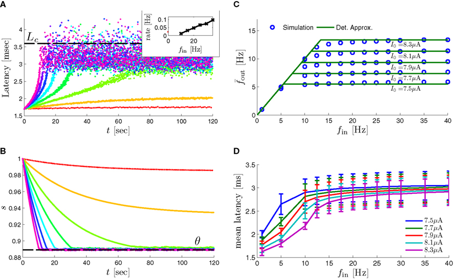
Figure 10. Stochastic HHS model – response dependency on f_in. Similar graphs to Figure 8. Note that due to the added noise the latency variance gradually increases during transients and is amplified during the intermittent mode (A,D), similarly to Figure 4A of Gal et al. (2010). In (C), the added noise makes the analytic approximation of the deterministic CBNM [equation (3.3)] no longer accurate, especially near An analytic result derived for the stochastic HHS model in our companion paper (not shown here), gives a better fit. N = 10⁷ in (A,B) and N = 10⁶ in (C,D).

The reasons that noise becomes very important in the HHS model are twofold. First, in the intermittent mode, the firing patterns of the neuron are dominated by small changes in the value of s near the threshold θ – and this near-threshold behavior, renders the noise term σ(s)ξ highly significant. Second, notice that since the noise term in equation (3.4) becomes large in comparison with the deterministic part of the equation, when the kinetic rates γ,δ are small. Therefore, since the rates of slow inactivation in the HHS model are about 10⁴-fold slower than the kinetic rates of the HH model, the noise term for s may become much more significant than that of the m, n, h variables. Specifically, in the fitted HHS model, we already found that in the intermittent mode Δs^± ∼ 10⁻⁴. Therefore, if for example there are N ≤ 10⁴ gating particles, then a conformation change in just few gating particles can potentially determine whether or not an AP will be generated.

In summary,

• Deterministic CBNMs (under our assumptions) can only generate regular firing patterns and non-variable latency transients, in contrast to the experimental results.

• The firing patterns during the intermittent mode in deterministic CBNMs are highly sensitive to perturbations, such as channel noise.

• When channel noise is added to the fitted HHS model, it generates highly irregular firing patterns (Figure 9D) and provides a better fit to the experimental latency fluctuations during the transient mode (Figure 10A).

Combining these observations we conclude that extending the deterministic CBNMs to stochastic CBNMs is a very plausible next step. However, keeping in mind our aim at mathematical tractability, we need analytic tools which are different from those used to analyze the deterministic model. Due to length considerations, we shall present these tools and the remaining results in a companion paper. Specifically, we will show how to calculate the mean and spectrum of the firing rate – and use these results to reproduce and explain the remaining experimental results.

4. Discussion

In this work we have developed a mathematical framework to analytically characterize the dynamics of deterministic conductance-based neuronal models of excitability under conditions of timescale separation and pulse-like inputs. A special simple case of the model studied, based on a single slow kinetic variable, allowed us to reproduce many of the qualitative and quantitative observations of Gal et al. (2010) in the stable, transient, and intermittent phases and to generate predictions, as summarized in more detail in the next paragraph. An extension to multiple channel types led to novel experimentally observed burst-like behavior. Attempting to extend the basic model in order to reproduce the specific details of the observed complex, irregular and “non-stationary” patterns that were observed experimentally, we argued for the necessity of incorporating ion channel stochasticity into the model. The analysis of such a model, requiring very different tools from those developed in the present paper, will be presented in a companion paper.

4.1. The HHS Model

In agreement with the conclusions of De Col et al. (2008), we showed that slow sodium inactivation alone (HHS model, section 2.2.1) can reproduce the different modes observed in Gal et al. (2010) – transient, stable, and intermittent, along with the critical frequency and the critical latency L_c. Using our simplification method (section 2.3), we were able to find exact expressions, directly linked to stimulation and biophysical parameters, that describe the neuronal response in all modes. Specifically, we found expressions describing the transient response of the neuron [equation (2.21)]; a simple piecewise linear and non-monotonic input-output relation for the mean firing rate as a function of stimulation frequency [equation (3.3) and Figure 8C] and also a simple description of the exact firing patterns in the intermittent mode directly linked to the firing rate (Figures 6A,B and 9A). The HHS model explains many of the phenomena observed in Gal et al. (2010): the dependence of the mean and variance of the latency on f_in (Figure 8D) and more specifically, the lack of dependence of L_c on f_in (Figure 8A); the linear increase of the transient rate of the latency mode with f_in [equation (3.1) and Figure 8A, inset] and the moderately decreasing response function in the intermittent mode [equation (3.3) and Figure 8C]. Using this result, we predicted that the slope of the response function, a, increases with the level of sub-threshold inactivation caused by the stimulation spike (γ_M) and argued for the possible existence of a second critical frequency above which the neuron does not generate APs (an unresponsive mode, which was observed for a similar setting in Kaplan et al. (1996), in cases where a is sufficiently high. Additionally, based on (see Figure A1), we predict that both and increase quadratically with I₀, that the latency decreases with I₀ (including L_c) and that the duration of the latency transients decreases with I₀.

We have not found other modeling work that deals with a similar setting to ours, namely excitable non-oscillatory neurons with slow kinetics under pulse stimulation. In most previous work either a constant current stimulation is used, neurons are oscillatory or slow kinetics are ignored. Therefore, it is somewhat difficult to compare this specific model with previous literature. However, we found that the non-monotonicity of the input/output relation, displays a similarity to that of a synapse with short term depression (de la Rocha and Parga, 2005), and that indeed becomes linear near similarly to the prediction of Ermentrout (1998), for CBNMs with a single slow adaptive variable.

4.2. Deterministic Conductance-Based Neuron Models

However, despite its merits, the HHS model fails to describe the firing patterns in the intermittent mode. This model can only produce very simple and stable periodic firing patterns (Figures 6A,B and 9A), in contrast with the irregular firing patterns of Gal et al. (2010). We attempted to circumvent this problem, by extending the HHS model with additional kinetic variables, representing channel activation/inactivation or concentration changes. Under the assumption of timescale separation [equation (2.9)] and the step-like behavior of the average kinetic rates [equation (2.12)], using our simplification methods (section 2.3), these models [equations (2.5–2.7)] remain amenable to analysis even when an arbitrary number of such kinetic variables is used. This allowed us again to find the different steady state modes (section 2.4) and closed-form expressions for the transient response [equation (2.21)], the firing rate [equation (2.24)] and the firing patterns [using equation (2.25)]. Using these methods we found, under the same assumptions, that the resulting firing patterns always remain periodic and stable (Figures 6C,D and 9B,C): in many cases identical to the simple firing patterns seen in the HHS model and in some cases (Figure 9A), when a certain analytical condition is fulfilled (section 2.4), additional “slow wave”-like “bursting” (Izhikevich, 2007) firing patterns appear (Figures 6D and 9C), as in some seen in Gal et al. (2010).

And so, even in the very general framework of deterministic CBNMs, it is impossible to reproduce the experimental observations regarding the fluctuations in latency transients or the irregular firing patterns in intermittent modes, given our assumptions. This necessarily entails that some of our assumptions must break down. What happens then? Can more complicated dynamics, or even chaos, be produced? It is generally known that chaotic dynamics are possible even in the basic HH model (Guckenheimer and Oliva, 2002) and in other models (Wang, 1993; Innocenti et al., 2007), in response to a constant current stimulation. Chaos was also shown to occur in the more relevant case of pulse stimulation in the Fitzhugh-Nagumo model (Kaplan et al., 1996) – although at rather high frequencies. In fact, if the timescale separation assumption [equation (2.9)] breaks down, we found that the original HHS model can produce chaos. Specifically, this occurs for I₀ = 7.7 μA, f_in = 35 Hz, when the assumption τ_r ≪ T no longer holds, and the fast HH variables V, m, n, h do not relax sufficiently quickly to a steady state between stimulation pulses. However, to our knowledge, in all these cases, chaos seems to be restricted to a limited (usually narrow) range of stimulus and model parameters. And so, it seems unlikely that irregular behavior will occur across a large variety of neurons, and for the entire range of stimulation parameters (I₀, f_in) that produce the intermittent mode. In fact, whenever f_in is sufficiently low so that τ_r ≪ min [T, τ_s ], the slow variables will again be uncoupled from the fast variables. It can be shown that this condition alone suffices to prevent chaotic dynamics (see section C). Therefore, if the observed irregularity occurs due to the breakdown of the timescale separation assumption [equation (2.9)], then this irregularity will not be robust to stimulus changes and will eventually disappear if f_in is low enough (note that I₀ might needed to be adjusted, so that the intermittent mode can be reached at this low value of f_in).

However, if the model kinetic timescales are not well separated and continuously span the full range of relevant stimulation periods, then the timescale separation condition cannot hold, even in its relaxed form. In this case, we cannot rule out the possibility that robust irregular dynamics may still emerge. This can also happen if any of the other assumptions are no longer valid. First, it might occur if the assumption related to the step-like behavior of the average kinetic rates [equation (2.12)] breaks down. Second, it is possible that we were too restrictive in assuming that the dynamics of s [equation (2.6)] are not directly coupled [as in equation (2.7), where is determined only by s_i, r, and not s, r]. Third, it might be that the conductance-based framework itself [equations (2.5 and 2.6)] is not general enough and must be extended to include other phenomena. We chose the latter option and extended the conductance-based framework by taking into account ion channel noise. In this way we maintained our ability to analytically study the model, thereby extending many of the results that were derived so far.

4.3. Ion Channel Noise

Since the observed irregularity in Gal et al. (2010) cannot be reproduced by adding any number of kinetic variables to the HHS model (under our assumptions), we argued that it is the result of the intrinsically stochastic nature of ion channels. Simulating this randomness, by adding channel noise to the HHS model, we found that it indeed reproduces the observed irregularity at short timescales (Figure 9D) and the variance increase in the latency fluctuations during the transient mode. Moreover, we found that channel noise has a strong impact on neuronal response, even when channel numbers (N) are much higher than previously considered. Specifically, in previous works (e.g., Fox and Lu, 1994; Rubinstein, 1995; Schneidman et al., 1998; White et al., 2000; Goldwyn et al., 2011) noise was demonstrated to be significant up to N ∼ 10⁴ or lower (except Rowat, 2007 with N ∼ 10⁵), while we showed it is highly significant even for channel numbers much larger than biophysically plausible (e.g., N ∼ 10⁷, Figure 10A). Such a high sensitivity to noise is the result of the slow kinetics and the near-threshold dynamics involved, as seen clearly from the simplified HHS model (section 3.3). A significant impact of the interaction between noise and slow kinetic variables was also reported recently by Schwalger et al. (2010).

Stochastic AP failures are not exclusive to the neuron, since synapses with low transmission probability are quite common (Thomson, 2000). Such a ubiquitous stochastic response may explain part of the puzzling irregular firing patterns of cortical cells (Softky and Koch, 1993). In a somewhat related matter, we note that the neuronal response discussed here is diametrically opposed to the popular notion of “large current fluctuations implies reliable response and vice versa” (Mainen and Sejnowski, 1995; Schneidman et al., 1998). If this notion was generally true then, given the short and strong pulse stimulation used in Gal et al. (2010), we should also expect a very reliable response. Yet, as we saw here, this is not the case in the intermittent mode – which is highly unreliable. Moreover, if a stochastic HHS model neuron is subjected to a constant current clamp, it would generate very regular and periodic firing patterns for N ∼ 10⁶ (not shown).

4.4. Neuronal Morphology

In this work we assumed that the neuron is a point element. However, cortical cells can have a complex spatial structure (Kriegstein and Dichter, 1983; Kandel et al., 2000) – which can be accounted for in the context of a CBNMs [equations (2.5–2.7)]. The spatial structure of the neuron is commonly modeled by dividing the neuron into several compartments representing different parts of the dendrites, soma, and axon. If a strong enough stimulation pulse arrives at one of the compartments (“initial compartment”) a signal propagates through the compartments until an AP is measured in the vicinity of another compartment (“final compartment”). Any such propagation event can change the excitability of each of the compartments it passes through (e.g., through slow sodium inactivation). When excitability reaches its threshold in one of the compartments, a conduction failure occurs. As we saw in this work, the excitability threshold depends on the internal variables of the compartments, and on the stimulation current entering the compartment (Figure 11). Conduction failure in a single compartment on the propagation path would result in no AP being measured in the final compartment. Such “critical compartments,” in which conduction failures occur, were already shown to appear in areas of impedance mismatch, such as axon branches (Grossman et al., 1979b; Debanne, 2004; Debanne et al., 2011). If this is the case here, and these branches are far from the initial compartment, then the observed AP failure rate should have a low sensitivity to I₀, and all our I₀-related results will not hold. However, if the AP failure rates change with I₀ as was predicted here (e.g., Figure A1C), then at least one of the critical compartments should be close to the stimulation area. The results of Wallach et al. (2011) indicate that this may be true at least in some cases. If the initial compartment is the only critical compartment (in which conduction failures occur), then all the results we’ve discussed here regarding AP firing patterns (and rate) hold in full.

FIGURE 11

Figure 11. AP propagation through neuronal compartments. After a stimulation is received in the initial compartment (1), it propagates through the neuronal compartments, until an AP is measured at the final compartment (4). This propagation could fail if the excitability of any of the compartments (e.g., 2) becomes low enough. This critical compartment (the “weakest link” in the propagation chain) will then determine the AP firing patterns. In contrast, the latency of AP propagating through the neuron is a sum of the latencies in all compartments on the path [equation (4.1)], and therefore depends on the excitability of all compartments.

In contrast to AP failures, which can depend only on the excitability of single critical compartment, the latency of an AP depends on the excitability of all compartments along the propagation path. And so, if AP latency is to be modeled in quantitatively correct manner, the spatial structure of the neuron must be considered. Specifically, the AP latency (measured from the beginning of a stimulation pulse to the time the AP peak is reached at the measuring electrode), is the sum of the propagation latencies along the propagation path,

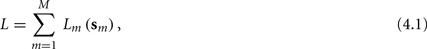
where each of these latencies is a direct function of that compartment’s excitability, as we saw in this work. This can be seen directly in the experimental results, as also pointed by Gal et al. (2010). For example, in Gal et al. (2010) Figure 2A, we clearly see that the AP waveform was measured only several millisecond after stimulation. This stands in contrasts with the AP waveform seen in a single compartment model which begins its rise immediately after the stimulation pulse (e.g., Figure 2 here or Figure 3A in Gal et al., 2010). Therefore this initial “pause” before AP measurement must result from the propagation time between the final and initial compartments. Taking equation (4.1) into account seems to explain why in our simulations (e.g., Figure 8A) the AP latency is significantly shorter than what was measured (e.g., Figure 4A in Gal et al., 2010). Also, assuming that the stochastic fluctuations in the latency response of each compartment are uncoupled, then according to equation (4.1), we get so the relative latency fluctuations will decrease with the number of compartments. This way, we would not have to use an unrealistic number of channels (N ∼ 10⁷) to get small magnitude latency fluctuations as in the experiment (Figure 10A). Finally, we comment that the AP amplitude and overall shape depends on the excitability of the final compartment. Its excitability is not necessarily coupled with the excitability of the critical compartments, due to the regenerative nature of the AP. Therefore, any long term changes in excitability or stimulation of the critical compartment might have little effect on the AP shape and amplitude. And so they should change very little during the experiment (Gal et al., 2010; Figure 5C).

4.5. What is the Relevant Physiological Input for Neuronal Models?

We concluded that the spatial structure of the neuron also affects our results. It may become even more important for in vivo neurons. To see why, recall that all our results were derived for the case of pulse stimulation at the physiological AP firing rate of cortical cells, as in Gal et al. (2010). For axonal compartments such a stimulation regime indeed resembles the physiologically relevant stimulation – an AP generated in the previous compartment. However, is sparse pulse stimulation also the physiologically relevant input regime of the soma and dendrites? The answer depends on the exact details of the spatial integration of synaptic inputs, and their temporal activation patterns. At first, a sparse input regime may seem unlikely given that neurons receive simultaneous inputs from about 10⁴ synapses. However, such a regime may seem more plausible if we recall that the mean firing rates of cortical neurons is low (less than 1 Hz according to Lee et al., 2006; see also Olshausen and Field, 2004 and references therein), and that in many cases incoming synaptic inputs do not reach the soma directly, but are integrated sequentially and non-linearly at several levels of dendritic compartments (Polsky et al., 2004; Larkum et al., 2009; Silver, 2010), so that each level may maintain a sparse input to the next level.

4.6. Functionality

Assuming that neuronal compartments indeed receive sparse input patterns, what could be the functional significance of the AP patterns observed in the intermittent mode? We end this paper by offering some speculations on this issue. As suggested here, these patterns are caused by the interaction between APs and the slow kinetic variables in the neurons (such as slow inactivation). In the sparse input regime characterizing the cortex, these slow kinetics allows two temporally separated inputs to interact with each other, thereby extending the timescale over which a computation could be performed beyond the several millisecond time window of the AP generation mechanism (Galán et al., 2008). Additionally, such a computation, performed through these slow kinetics, will be more robust to millisecond fluctuations (as seen in Gal et al., 2010; Figures 4D–F) in the input timing, than computations performed solely through fast kinetics. However, as we mentioned previously, such slow kinetics are more strongly affected by ion channel noise. This is not necessarily a disadvantage. For example, noise can increase signal to noise ratio via stochastic resonance (Van den Broeck et al., 1994; Gammaitoni et al., 1998; Mcdonnell and Ward, 2011), reduce the network sensitivity to perturbations (Molgedey et al., 1992), enable escape from local minima in optimization (Kirkpatrick et al., 1983), improve fault tolerance, learning speed, and generalization ability in neural networks (Murray and Edwards, 1993, 1994; Jim et al., 1996; Fiete and Seung, 2006) and serve other beneficial purposes in many cases (Motwani and Raghavan, 1996).

Conflict of Interest Statement

The authors declare that the research was conducted in the absence of any commercial or financial relationships that could be construed as a potential conflict of interest.

Acknowledgments

The authors are grateful to E. Braun, N. Brenner, Y. Elhanati, A. Gal, Y. Kafri, S. Marom, and A. Wallach for many insightful discussions. This work was partially supported by grant No. 665/08 from the Israel Science Foundation.

Footnote

1. ^MATLAB code available on http://webee.technion.ac.il/∼rmeir/SoudryMeir2011Deterministic_code.rar

References

Bean, B. P. (2007). The action potential in mammalian central neurons. Nat. Rev. Neurosci. 8, 451–465.

Pubmed Abstract | Pubmed Full Text | CrossRef Full Text

Blondel, V. D., Bournez, O., Koiran, P., Papadimitriou, C., and Tsitsiklis, J. N. (1999). Deciding stability and mortality of piecewise affine dynamical systems. Theor. Comp. Sci. 255, 687–696.

CrossRef Full Text

Cannon, R. C., O’Donnell, C., and Nolan, M. F. (2010). Stochastic ion channel gating in dendritic neurons: morphology dependence and probabilistic synaptic activation of dendritic spikes. PLoS Comput. Biol. 6, 18.

CrossRef Full Text

Carelli, P. V., Reyes, M. B., Sartorelli, J. C., and Pinto, R. D. (2005). Whole cell stochastic model reproduces the irregularities found in the membrane potential of bursting neurons. J. Neurophysiol. 94, 1169–1179.

Pubmed Abstract | Pubmed Full Text | CrossRef Full Text

Chandler, W. K., and Meves, H. (1970). Slow changes in membrane permeability and long-lasting action potentials in axons perfused with fluoride solutions. J. Physiol. (Lond.) 211, 707.

Pubmed Abstract | Pubmed Full Text

Chow, C., and White, J. A. (1996). Spontaneous action potentials due to channel fluctuations. Biophys. J. 71, 3013–3021.

Pubmed Abstract | Pubmed Full Text | CrossRef Full Text

De Col, R., Messlinger, K., and Carr, R. W. (2008). Conduction velocity is regulated by sodium channel inactivation in unmyelinated axons innervating the rat cranial meninges. J. Physiol. (Lond.) 586, 1089.

Pubmed Abstract | Pubmed Full Text | CrossRef Full Text

de la Rocha, J., and Parga, N. (2005). Short-term synaptic depression causes a non-monotonic response to correlated stimuli. J. Neurosci. 25, 8416–8431.

Pubmed Abstract | Pubmed Full Text | CrossRef Full Text

De Schutter, E. (2010). Computational Modeling Methods for Neuroscientists, Cambridge: The MIT Press.

Debanne, D. (2004). Information processing in the axon. Nat. Rev. Neurosci. 5, 304–316.

Pubmed Abstract | Pubmed Full Text | CrossRef Full Text

Debanne, D., Campanac, E., Bialowas, A., and Carlier, E. (2011). Axon physiology. Physiol. Rev. 555–602.

Pubmed Abstract | Pubmed Full Text | CrossRef Full Text

Di Bernardo, M. (2008). Piecewise-Smooth Dynamical Systems: Theory and Applications, Vol. 163. London: Springer Verlag.

Diba, K., Lester, H. A., and Koch, C. (2004). Intrinsic noise in cultured hippocampal neurons: experiment and modeling. J. Neurosci. 24, 9723–9733.

Pubmed Abstract | Pubmed Full Text | CrossRef Full Text

Dorval, A. D., and White, J. A. (2005). Channel noise is essential for perithreshold oscillations in entorhinal stellate neurons. J. Neurosci. 25, 10025–10028.

Pubmed Abstract | Pubmed Full Text | CrossRef Full Text

Ellerkmann, R. K., Riazanski, V., Elger, C. E., Urban, B. W., and Beck, H. (2001). Slow recovery from inactivation regulates the availability of voltage-dependent Na+ channels in hippocampal granule cells, hilar neurons and basket cells. J. Physiol. (Lond.) 532, 385.

Pubmed Abstract | Pubmed Full Text | CrossRef Full Text

Ermentrout, B. (1996). Type I membranes, phase resetting curves, and synchrony. Neural Comput. 8, 979–1001.

Pubmed Abstract | Pubmed Full Text | CrossRef Full Text

Ermentrout, B. (1998). Linearization of F-I curves by adaptation. Neural Comput. 10, 1721–1729.

Pubmed Abstract | Pubmed Full Text | CrossRef Full Text

Ermentrout, B., and Terman, D. H. (2010). Mathematical Foundations of Neuroscience (New York: Springer).

Faisal, A. A. (2009). “Stochastic simulation of neurons, axons and action potentials,” in Stochastic Methods in Neuroscience eds C. Laing, and J. L. Gabrieal (New York: Oxford University Press), 297–343.

Faisal, A. A., and Laughlin, S. B. (2007). Stochastic simulations on the reliability of action potential propagation in thin axons. PLoS Comput. Biol. 3, e79.

CrossRef Full Text

Faisal, A. A., Luc Selen, P. J., and Wolpert, D. M. (2008). Noise in the nervous system. Nat. Rev. Neurosci. 9, 292–303.

Pubmed Abstract | Pubmed Full Text | CrossRef Full Text

Fiete, I., and Seung, H. (2006). Gradient learning in spiking neural networks by dynamic perturbation of conductances. Phys. Rev. Lett. 97, 48014.

CrossRef Full Text

Fitzhugh, R. (1961). Impulses and physiological states in theoretical models of nerve membrane. Biophys. J. 1, 445–466.

Pubmed Abstract | Pubmed Full Text | CrossRef Full Text

Fleidervish, I. A., Friedman, A., and Gutnick, M. J. (1996). Slow inactivation of Na+ current and slow cumulative spike adaptation in mouse and guinea-pig neocortical neurones in slices. J. Physiol. 493, 83–97.

Pubmed Abstract | Pubmed Full Text

Fleidervish, I. A., Lasser-Ross, N., Gutnick, M. J., and Ross, W. N. (2010). Na+ imaging reveals little difference in action potential-evoked Na+ influx between axon and soma. Nat. Neurosci. 13, 852–860.

Pubmed Abstract | Pubmed Full Text | CrossRef Full Text

Fox, R., and Lu, Y. (1994). Emergent collective behavior in large numbers of globally coupled independently stochastic ion channels. Phys. Rev. E 49, 3421–3431.

CrossRef Full Text

Gal, A., Eytan, D., Wallach, A., Sandler, M., Schiller, J., and Marom, S. (2010). Dynamics of excitability over extended timescales in cultured cortical neurons. J. Neurosci. 30, 16332–16342.

Pubmed Abstract | Pubmed Full Text | CrossRef Full Text

Galán, R. F., Ermentrout, B., and Urban, N. N. (2008). Optimal time scale for spike-time reliability: theory, simulations, and experiments. J. Neurophysiol. 99, 277–283.

Pubmed Abstract | Pubmed Full Text | CrossRef Full Text

Gammaitoni, L., Nazionale, I., Fisica, D., Perugia, S., Perugia, I., Augsburg, D., Jung, P., Marchesoni, F., and Camerino, I. (1998). Stochastic resonance. Rev. Mod. Phys. 70, 23–287.

CrossRef Full Text

Gerstner, W., and Kistler, W. M. (2002). Spiking Neuron Models: Single Neurons, Populations, Plasticity, Cambridge: Cambridge University Press.

Goldwyn, J., Imennov, N., Famulare, M., and Shea-Brown, E. (2011). Stochastic differential equation models for ion channel noise in Hodgkin-Huxley neurons. Phys. Rev. E 83, 041908.

CrossRef Full Text

Griffiths, R. E., and Pernarowski, M. (2006). Return map characterizations for a model of bursting with two slow variables. SIAM J. Appl. Math. 66, 1917–1948.

CrossRef Full Text

Grossman, B. Y. Y., Parnas, I., and Spira, M. E. (1979a). Differential conduction block in branches of a bifurcating axon. J. Physiol. (Lond.) 295, 283–305.

Grossman, B. Y. Y., Parnas, I., and Spira, M. E. (1979b). Mechanisms involved in differential conduction of potentials at high frequency in a branching axon. J. Physiol. (Lond.) 295, 307–322.

Guckenheimer, J., and Oliva, R. A. (2002). Chaos in the Hodgkin–Huxley Model. SIAM. J. Appl. Dyn. Syst. 1, 105.

CrossRef Full Text

Henze, D. A., Borhegyi, Z., Csicsvari, J., Mamiya, A., Harris, K. D., and Buzsáki, G. (2011). Intracellular features predicted by extracellular recordings in the hippocampus in vivo. J. Neurophysiol. 84, 390–400.

Hille, B. (2001). Ion Channels of Excitable Membranes, 3rd Edn. Sunderland, MA: Sinauer Associates.

Hodgkin, A. L., and Huxley, A. F. (1952). A quantitative description of membrane current and its application to conduction and excitation in nerve. J. Physiol. (Lond.) 117, 500.

Pubmed Abstract | Pubmed Full Text

Hoshi, T., and Zagotta, W. N. (1991). Two types of inactivation in Shaker K+ channels: effects of alterations in the carboxy-terminal region. Neuron 7, 547–556.

Pubmed Abstract | Pubmed Full Text | CrossRef Full Text

Ibarz, B., Casado, J. M., and M. Sanjuán, A. F. (2011). Map-based models in neuronal dynamics. Phys. Rep. 501, 1–74.

CrossRef Full Text

Innocenti, G., Morelli, A., Genesio, R., and Torcini, A. (2007). Dynamical phases of the Hindmarsh-Rose neuronal model: studies of the transition from bursting to spiking chaos. Chaos 17, 043128.

Pubmed Abstract | Pubmed Full Text | CrossRef Full Text

Izhikevich, E. M. (2007). Dynamical Systems in Neuroscience. Cambridge, MA: MIT Press.

Jim, K. C., Giles, C. L., and Horne, B. G. (1996). An analysis of noise in recurrent neural networks: convergence and generalization. IEEE Trans. Neural Netw. 7, 1424–1438.

Pubmed Abstract | Pubmed Full Text | CrossRef Full Text

Juan, M., Yu-Ye, L., Chun-Ling, W., Ming-Hao, Y., Hua-Guang, G., Shi-Xian, Q., and Wei, R. (2010). Interpreting a period-adding bifurcation scenario in neural bursting patterns using border-collision bifurcation in a discontinuous map of a slow control variable. Chin. Phys. B 19, 80513.

CrossRef Full Text

Kandel, E. R., Schwartz, J. H., Jessell, T. M., Mack, S., and Dodd, J. (2000). Principles of Neural Science, Vol. 3, 4th Edn. New York: Elsevier.

Kaplan, D. T., Clay, J. R., Manning, T., Glass, L., Guevara, M. R., and Shrier, A. (1996). Subthreshold dynamics in periodically stimulated squid giant axons. Phys. Rev. Lett. 76, 4074–4077.

Pubmed Abstract | Pubmed Full Text | CrossRef Full Text

Keener, J. P. (1980). Chaotic behavior in piecewise continuous difference equations. Trans. Am. Math. Soc. 261, 589–604.

CrossRef Full Text

Kirkpatrick, S., Gelatt, C. D., and Vecchi, M. P. (1983). Optimization by simulated annealing. Science 22, 671.

CrossRef Full Text

Koch, C., and Schutter, E. (2004). Biophysics of Computation: Information Processing in Single Neurons, New York: Oxford University Press.

Koch, C., and Segev, I. (1989). Methods in Neuronal Modeling: From Ions to Networks, Vol. 484, 2nd Edn. Cambridge: MIT press.

Kole, M. H. P., Ilschner, S. U., Kampa, B. M., Williams, S. R., Ruben, P. C., and Stuart, G. J. (2008). Action potential generation requires a high sodium channel density in the axon initial segment. Nat. Neurosci. 110, 178–186.

CrossRef Full Text

Kriegstein, A. R., and Dichter, M. A. (1983). Morphological classification of rat cortical neurons in cell culture. J. Neurosci. 3, 1634.

Pubmed Abstract | Pubmed Full Text

Larkum, M. E., Nevian, T., Sandler, M., Polsky, A., and Schiller, J. (2009). Synaptic integration in tuft dendrites of layer 5 pyramidal neurons: a new unifying principle. Science 325, 756–760.

Pubmed Abstract | Pubmed Full Text | CrossRef Full Text

Lee, A. K., Manns, I. D., Sakmann, B., and Brecht, M. (2006). Whole-cell recordings in freely moving rats. Neuron 51, 399–407.

Pubmed Abstract | Pubmed Full Text | CrossRef Full Text

Linaro, D., Storace, M., and Giugliano, M. (2011). Accurate and fast simulation of channel noise in conductance-based model neurons by diffusion approximation. PLoS Comput. Biol. 7, e1001102.

CrossRef Full Text

Mainen, Z. F., and Sejnowski, T. J. (1995). Reliability of spike timing in neocortical neurons. Science 268, 1503.

Pubmed Abstract | Pubmed Full Text | CrossRef Full Text

Marom, S. (2010). Neural timescales or lack thereof. Prog. Neurobiol. 90, 16–28.

Pubmed Abstract | Pubmed Full Text | CrossRef Full Text

Marom, S., and Abbott, L. F. (1994). Modeling state-dependent inactivation of membrane currents. Biophys. J. 67, 515–520.

Pubmed Abstract | Pubmed Full Text | CrossRef Full Text

Mcdonnell, M. D., and Ward, L. M. (2011). The benefits of noise in neural systems: bridging theory and experiment. Nat. Rev. Neurosci. 12, 415–426.

Pubmed Abstract | Pubmed Full Text | CrossRef Full Text

Medvedev, G. (2005). Reduction of a model of an excitable cell to a one-dimensional map. Physica D 202, 37–59.

CrossRef Full Text

Molgedey, L., Schuchhardt, J., and Schuster, H. G. (1992). Suppressing chaos in neural networks by noise. Phys. Rev. Lett. 69, 3717–3719.

Pubmed Abstract | Pubmed Full Text | CrossRef Full Text

Morris, C., and Lecar, H. (1981). Voltage oscillations in the barnacle giant muscle fiber. Biophys. J. 35, 193–213.

Pubmed Abstract | Pubmed Full Text | CrossRef Full Text

Motwani, R., and Raghavan, P. (1996). Randomized Algorithms, Cambridge, UK: Cambridge University Press.

Murray, A. F., and Edwards, P. J. (1993). Synaptic weight noise during multilayer perceptron training: fault tolerance and training improvements. IEEE Trans. Neural Netw. 4, 722–725.

Pubmed Abstract | Pubmed Full Text | CrossRef Full Text

Murray, A. F., and Edwards, P. J. (1994). Enhanced MLP performance and fault tolerance resulting from synaptic weight noise during training. IEEE Trans. Neural Netw. 5, 792–802.

Pubmed Abstract | Pubmed Full Text | CrossRef Full Text

Olshausen, B. A., and Field, D. J. (2004). Sparse coding of sensory inputs. Curr. Opin. Neurobiol. 14, 481–487.

Pubmed Abstract | Pubmed Full Text | CrossRef Full Text

Polsky, A., Mel, B., and Schiller, J. (2004). Computational subunits in thin dendrites of pyramidal cells. Nat. Neurosci. 7, 621–627.

Pubmed Abstract | Pubmed Full Text | CrossRef Full Text

Pospischil, M., Toledo-Rodriguez, M., Monier, C., Piwkowska, Z., Bal, T., Frégnac, Y., Markram, H., and Destexhe, A. (2008). Minimal Hodgkin-Huxley type models for different classes of cortical and thalamic neurons. Biol. Cybern. 99, 427–441.

Pubmed Abstract | Pubmed Full Text | CrossRef Full Text

Powers, R. K., Sawczuk, A., Musick, J. R., and Binder, M. D. (1999). Multiple mechanisms of spike-frequency adaptation in motoneurones. J. Physiol. Paris 93, 101–114.

Pubmed Abstract | Pubmed Full Text | CrossRef Full Text

Rowat, P. (2007). Interspike interval statistics in the stochastic Hodgkin-Huxley model: coexistence of gamma frequency bursts and highly irregular firing. Neural Comput. 19, 1215–1250.

Pubmed Abstract | Pubmed Full Text | CrossRef Full Text

Rubinstein, J. (1995). Threshold fluctuations in an N sodium channel model of the node of Ranvier. Biophys. J. 68, 779–785.

Pubmed Abstract | Pubmed Full Text | CrossRef Full Text

Rudy, B. Y. B. (1978). Slow inactivation of the sodium conductance in squid giant axons. Pronase resistance. J. Physiol. 283, 1003.

Schneidman, E., Freedman, B., and Segev, I. (1998). Ion channel stochasticity may be critical in determining the reliability and precision of spike timing. Neural Comput. 10, 1679–1703.

Pubmed Abstract | Pubmed Full Text | CrossRef Full Text

Schwalger, T., Fisch, K., Benda, J., and Lindner, B. (2010). How noisy adaptation of neurons shapes interspike interval histograms and correlations. PLoS Comput. Biol. 6, e1001026.

CrossRef Full Text

Silver, R. A. (2010). Neuronal arithmetic. Nat. Rev. Neurosci. 11, 474–489.

Pubmed Abstract | Pubmed Full Text | CrossRef Full Text

Sjostrom, P. J., Rancz, E. A., Roth, A., and Häusser, M. (2008). Dendritic excitability and synaptic plasticity. Physiol. Rev. 88, 769–840.

Pubmed Abstract | Pubmed Full Text | CrossRef Full Text

Softky, W. R., and Koch, C. (1993). The highly irregular firing of cortical cells is inconsistent with temporal integration of random EPSPs. J. Neurosci. 13, 334.

Pubmed Abstract | Pubmed Full Text

Soudry, D., and Meir, R. (2010). History dependent dynamics in a generic model of ion channels – an analytic study. Front. Comput. Neurosci. 4:3.

CrossRef Full Text

Steinmetz, P. N., Manwani, A., Koch, C., London, M., and Segev, I. (2000). Subthreshold voltage noise due to channel fluctuations in active neuronal membranes. J. Comput. Neurosci. 9, 133–148.

Pubmed Abstract | Pubmed Full Text | CrossRef Full Text

Strogatz, S. H. (1994). Nonlinear Dynamics and Chaos, New York: Perseus Books.

Thompson, J. M. T., and Stewart, H. B. (2002). Nonlinear Dynamics and Chaos. 2nd Edn. West Sussex: John Wiley & Sons Inc.

Thomson, A. M. (2000). Facilitation, augmentation and potentiation at central synapses. Trends Neurosci. 230, 305–312.

CrossRef Full Text

Toib, A., Lyakhov, V., and Marom, S. (1998). Interaction between duration of activity and time course of recovery from slow inactivation in mammalian brain Na+ channels. J. Neurosci. 18, 1893.

Pubmed Abstract | Pubmed Full Text

Touboul, J., and Faugeras, O. (2007). The spikes trains probability distributions: a stochastic calculus approach. J. Physiol. Paris 101, 78–98.

Pubmed Abstract | Pubmed Full Text | CrossRef Full Text

Tramontana, F., Gardini, L., and Agliari, A. (2010). Endogenous cycles in discontinuous growth models. Math. Comput. Simul. 81, 1–25.

CrossRef Full Text

Van den Broeck, C., Parrondo, J. M. R., and Toral, R. (1994). Noise-induced nonequilibrium phase transition. Phys. Rev. Lett. 73, 3395–3398.

Pubmed Abstract | Pubmed Full Text | CrossRef Full Text

Wallach, A., Eytan, D., Gal, A., Zrenner, C., and Marom, S. (2011). Neuronal response clamp. Front. Neuroeng. 4, 1–10.

Pubmed Abstract | Pubmed Full Text | CrossRef Full Text

Wang, X. J. (1993). Genesis of bursting oscillations in the Hindmarsh-Rose model and homoclinicity to a chaotic saddle. Physica D 62, 263–274.

CrossRef Full Text

White, J. A., Klink, R., Alonso, A., and Kay, A. R. (1998). Noise from voltage-gated ion channels may influence neuronal dynamics in the entorhinal cortex. J. Neurophysiol. 80, 262–269.

Pubmed Abstract | Pubmed Full Text

White, J. A., Rubinstein, J. T., and Kay, A. R. (2000). Channel noise in neurons. Trends Neurosci. 23, 131–137.

Pubmed Abstract | Pubmed Full Text | CrossRef Full Text

Wiggins, S. (2003). Introduction to Applied Nonlinear Dynamical Systems and Chaos, New York.

Appendix

A. Stability and Uniqueness of the Intermittent Steady State

For completeness, we explain in this section some of the properties of the limit cycle in s during the intermittent mode, in the context of our simplified model. Assume that the model parameters are chosen so that eventually the intermittent steady state is reached. In this case, according to equation (2.14), the discrete vector-valued map

is given by

Expressed in vector notation, we have

where G_± are diagonal matrices with eigenvalues inside the unit circle (the latter property follows from the assumption that ).

First, note that this map has no fixed point (a point s* for which s* = g(s*)), otherwise the system would be in the stable, bi-stable, or unresponsive mode, rather than the intermittent mode. In order to consider cycles, we define the iterated map recursively for all n ≥ 0, gⁿ(s) = g(gⁿ⁻¹(s)), where g⁰(s) = s. Assume there exists a finite limit cycle, i.e., there exists a p > 1 so that for some This means that a p-long periodic limit cycle exists for this map (i.e., ). We also assume that Θ ∩ P = ∅, since the complementary event occurs only for a measure zero set of parameters. The finiteness of the limit cycle in this case (contracting maps) was proved by Keener (1980) for the 1D case, for all but a measure zero choice of parameters. We are not aware of a generalization of this result to higher-dimensional systems, but simulations seem to confirm that this remains true.

A.1. Local Stability of P

Assume the system is 1D. A generalization of the following result to higher dimensions is straightforward.

The limit cycle P is locally stable if and only if (Strogatz, 1994). By the chain rule, this is true if and only if

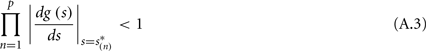
Since

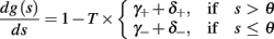
and T(γ_± + δ_±) < 1, it follows that for all s, |dg(s)/ds| < 1. This implies that condition A.3 is fulfilled, and so P is stable. Note that since we assumed that θ ∉ P, we can always choose a neighborhood of all the points in P that does not contain θ, and thus the condition 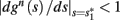indeed implies stability (we do not have to worry about the discontinuity at s = θ).

A.2. Uniqueness and Global Stability of P

Assume the system is 1D. We now prove the uniqueness of P in the intermittent mode, implying that there is no other attractor A so that P ∩ A ≠ P. We are not aware of a generalization of the following result to higher dimensions.

Assume by contradiction that there are two different attractors A₁ and A₂. For each attractor A_i, by its definition (Wiggins, 2003, Chapter 8.2) there exists an open set U_i (a “trapping region”) so that ∀n ≥ 0: gⁿ (U_i) ⊂ U_i and ∩_{n ≥ 0} gⁿ(U_i) = A_i, where The basin of attraction of A_i is defined as 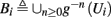where . As implied by the definition, B₁ ∩ B₂ = ∅. Assume that θ ∉ B₁. This implies that ∀n ≥ 0: θ ∉ g⁻ⁿ (U₁). Therefore, using the fact that U₁ is an open set and g(s) is a continuous function anywhere except in θ, by the topological definition of a continuous function (which states that the inverse image of any open set must be an open set), we arrive to the conclusion that ∀n ≥ 0: g⁻ⁿ (U₁) is also open. This means that B_i ≜ ∪_n≥0g⁻ⁿ(U_i) is also open, as the union of open sets. Since B₁ ∈ [0,1] then as an open set it must be the union of disjoint open intervals of the form (a, b) and perhaps also half-open intervals of the form [0,b) or (a,1].

Assume that B₁ contains at least one open interval of the form (a, b). We choose some c ∈ (a, b). Since θ ∉ B₁ then ∀n ≥ 0: θ ∉ gⁿ[c, b) and so gⁿ(s) is continuous, differentiable, and monotonically increasing in [c, b), as the composition of such functions. Since g(s) is left-continuous everywhere and gⁿ(s) is monotonically increasing in [c, b), then gⁿ(s) is also continuous on [c, b]. Therefore, we can now use the mean value theorem, and state that there exists some d ∈ (c, b) so that

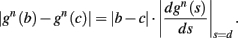
Using the chain rule again we get

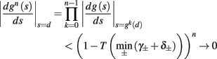
as n → ∞ This implies that 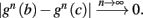But since c ∈ B₁, then and so - which contradicts our assumption that b ∉ B₁. Therefore B₁ does not contain any interval of the form (a, b). Using identical reasoning, any interval of the form [0,b) is also disqualified from being in B₁. The only remaining possibility is that B₁ is of the form (a,1] where a > θ. But this is also impossible if we are in the intermittent mode (where the dynamics always cross the threshold eventually) – since then there exists an e so that g(a + ∊) < a and so g(a + ∊) ∉ B₁ even though a + ∊ ∈ B₁, which means that B₁ cannot be a basin of attraction (if instead we are in the bi-stable mode then we can have two basins of attraction – [0, θ] and [θ, 1]). Therefore, there cannot be any basin of attraction that does not contain θ. This means there is only a single basin of attraction, and that it must contain θ.

Therefore P is the only attractor, and so it is globally attracting.

B. Model Assumptions

In this section we examine more closely the two main assumptions we used to generate and analyze our simplified model. For simplicity and numerical concreteness, we consider only the fitted HHS model, in which s = s, a scalar variable, and E(s) = θ. Generalization to other models should be straightforward.

B.1. Step Function Approximation for the Kinetic Rates

In this section we examine closely the step approximation we used for the average kinetic rate [used in equations (2.12 and 2.20)]. Namely, we want to quantify more accurately the limits of this approximation.

How does equation (2.12) affect the AP firing patterns? Without this approximation the discrete mapping g(s) [equation ((A.2))] becomes

The difference between the map in the approximated and non-approximated case can be seen in Figure A4B. In the non-approximated map g(s) changes gradually over a “threshold interval” of width e that contains a single fixed point (in which s_n = s_n+1), while the approximated map has no fixed points. Also, away from the threshold, the slopes of the non-approximated map are somewhat smaller than in the approximated map, since is monotonically increasing.

First we explore the stability of the fixed point. This depends on the value of

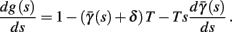
Notice that 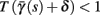since s is “slow” (with small kinetic rates), while can be large only in the threshold interval (Figure A4A). As long as |dg(s)/ds|_s=θ > 1 the fixed point is unstable (Strogatz, 1994). However, if the kinetic rates γ, δ are very small we might get |dg(s)/ds|_s=θ < 1. In this case, the system will have a stable fixed point and a low-amplitude (“weak AP-response”) AP will be produced in each period. If this is not the case, and if the fixed point is unstable, then the step approximation for g(s) will give similar results to the non-approximated version in the stability analysis (section A.1), given two more conditions. First, the width of the threshold interval, η (Figure A4A), is small enough so no point in the limit cycles falls directly into it. Second, 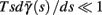so the map remains contracting and the limit cycle remains stable.

Another result that used the step-like behavior of the kinetic rates is the continuous-time differential equation which we used to derive the behavior of s in the transient phase in equation (2.20). This seems like an adequate approximation in the cases we checked (Figure 7 (middle)). To increase accuracy, we can avoid the approximation, and just use

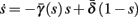
instead. However, in this case we cannot derive the analytic solution [equation (2.21)] and the resulting linear scaling of transients [equation (3.1)].

Finally, one might ask why the step-like shape arises at all in the context of the average kinetic rates. There are three properties of HHS which, given together, enhance this:

1. The sigmoidal form of γ(V), δ(V) which reduces the sensitivity to changes in the amplitude of the AP or the resting potential.

2. The shape of the AP is relatively insensitive to s.

3. The resting voltage is relatively insensitive to s.

Whenever a conductance-based model has these properties, we expect the step approximation to remain valid.

B.2. Timescale Separation Assumption

In the main text, in order to develop the simplified model, we used the timescale separation assumption [equation (2.9)], which is actually based on two different assumptions, namely τ_s ≫ T and τ_r ≪ T. The condition τ_s ≫ T is straightforward to understand and was applied using standard perturbation theory [in equation (2.10)] and similarly the use of the condition τ_r ≪ T in the context of section 2.3. However, our use of the condition τ_r ≪ T in the definition of E(s) needs be further clarified. In order to simplify the HHS model we assumed that an AP will be produced after a stimulation pulse if and only if s > θ. However, if T < τ_r, θ may change if an AP was generated by the previous stimulation pulse through the HH variables therefore θ = θ(r). We denote the HH (resting) steady state by (note that in general r₀ may depend on s, but this is not relevant here). Our model assumption T > τ_r implies that when a stimulation pulse is given is small. However, small in comparison to what? If, for example, we want our model to give accurate results regarding the firing patterns in the intermittent mode (when s is near θ), then we need to demand

where Δs^± are given by equation (2.25) for the HHS case

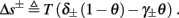
Assume that a stimulation was given at time t = 0 and an AP was produced. For which values of T is the requirement B.2 fulfilled? As can be seen in Figure 2, the AP has a stereotypical timescale of τ_AP (≈10 ms) in which r are far from the steady state r₀. After that, r relax to r₀ with the difference Δr = r − r₀ remaining small. Since Δr is small, we can linearize the HH equations near and obtain

where A is a constant 4 × 4 matrix. Solving this equation we obtain

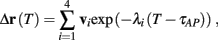
where λ_i are the eigenvalues of A and v_i are some vectors, depending on the initial conditions. For our fitted HH model, we can calculate λ₁ = 5.44 kHz, λ_2,3 = 0.36 ± 0.86i kHz, λ₄ = 0.24 kHz. For T > τ_AP, Δr is small, so we can approximate to first order Δθ ≈ w^⊤Δr where w is some constant vector. Denoting c_i = w^⊤v_i, we obtain the condition

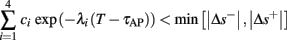
We can further approximate if λ₄(T − τ_AP) ≫ 1, since then Δθ ≈ c₄ exp (− λ₄(T − τ_AP)), where c₄ is some constant in the range [0, min (θ, 1 − θ)]. Using this approximation we obtain

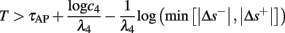
For example, using a higher bound by setting c₄ = min (θ, 1 − θ), and solving for parameter values of the fitted HHS model obtained for I₀ = 10 μA (Figure 4), we obtain T > 47.8 ms (or f_in < 21.4 Hz). Above this bound, the approximation τ_r ≪ T is guaranteed to be correct. However, it gives relatively large safety margins, since our numerical results show that our simplified fitted HHS model seemed to hold up well for f_in < 30 Hz as can bee seen in Figures 8A,C and 9A (also, f_in < 30 Hz for the original HHS model as can bee seen in Figure A2A).

C. Relaxation of Assumptions

In this section we relax the timescale separation assumption [equation (2.9)] to τ_r ≪ min[T, τ_s], and instead of requiring that h_i(r, s_i) is linear [equation (2.7)], we only require that h_i(r, s_i) is a monotonic function of s_i.

We show that even under these milder assumptions the model remains non-chaotic and can produce only stable firing patterns (except perhaps in a parameter set of measure zero), by proving that the simplified discrete mapping g(s) [equation ((A.2))] remains diagonal and contracting (namely, |dg_i(s)/ds_i| < 1, and |dg_i(s)/ds_j| = 0 for all i≠j) whenever s is not on Θ.

We denote a_i ≜ s_i(t), b_i ≜ s_i(t + τ_r), c_i ≜ s_i(t + T). The system dynamics generate mappings b = f(a), c = e(b). We aim to prove that all the eigenvalues of g(a) = e(f(a)) are inside the unit circle.

Using equations (2.6 and 2.7) we write

where

where in the last line we made the assumption on the step-like behavior of the dynamics: is insensitive to changes in caused by changes in s(t), except near the threshold E(s) = 0, while is completely insensitive to changes in caused by changes in s(t). Therefore, we can write for all u ∈ [t + τ_r, t + T] and get

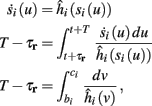
Differentiating with respect to b_i we get

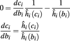
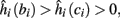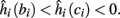now since h_i(r, s_i) are monotonic, and since s is bounded, must be monotonically decreasing (if it were increasing then the system will be unstable and s will diverge). In any case, the system dynamics evolve so Therefore, if then and if then And so,

In summary, if a_i ∉ Θ

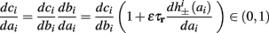
since ∊τ_r ≪ 1. Also

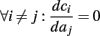
therefore g(a) is diagonal and contracting, and so any finite limit cycle (which does not touch the threshold) is stable. Note that we demand a_i ∉ Θ (a_i ∈ Θ in a parameter set of measure zero), since if a_i ∈ Θ, then is discontinuous so is ill-defined.

FIGURE A1

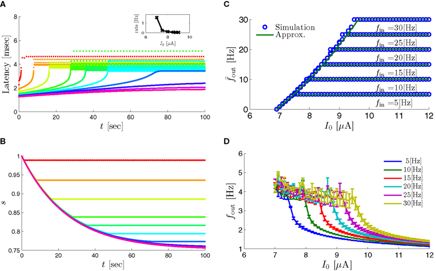
Figure A1. Dependency on stimulation amplitude, I₀, in the fitted HHS model – (A) Spike latency as a function of time from stimulation onset (each color designates a different stimulation rate): stimulation at f_in = 25 Hz and I₀ = 7, 7.5, 8, 8.5, 8.75, 9, 9.25, 9.5, 9.75, 10 μA (red, orange…,); The transient slows down when I₀ is increased, and both initial and critical latencies change. Inset: the rate indeed decreases with I₀, and there exist two critical currents: which is the minimal current to generate an AP (here ) and which is the maximal current for which intermittent mode is reached (here ). For the steady state is the stable mode. These results can be explained by (B) the sodium availability trace s(t) (using same color code as in A), where we see that when I₀ is increased then θ is decreased, while the transient rate of s is hardly affected. (C) Steady state firing rate is 0 for 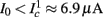for all f_in. It then increases quadratically in I₀ during the intermittent mode, until saturates when the stable mode is reached – at which depends on f_in. (D) Steady state latency dependence on I₀. For f_in = 25 Hz, the mean latency at steady state always decreases as a function of I₀. This mainly occurs since the latency function decreases with I₀ (Figure 3). However, during the intermittent mode, L ≈ L(θ), while θ decreases with current. Since L(s) is decreasing, this makes the decline of L in the intermittent mode less steep than in the stable mode, where and does not change with I₀. Here we also see that the latency fluctuations in the intermittent mode are much larger than in the stable mode.

FIGURE A2

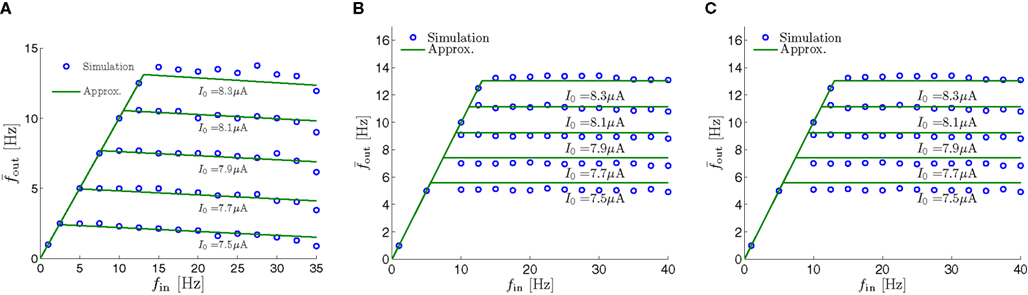
Figure A2. Dependency of on f_in for different models. (A) Original HHS model (t₀ = 1 ms). Notice that with a > 0 for 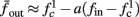(intermittent mode). (B) HHSAP. (C) HHSIP.

FIGURE A3

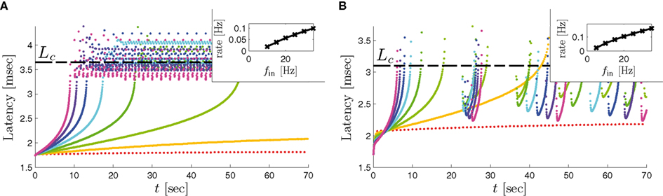
Figure A3. Transient mode in the HHSIP model. Similar graphs as in Figure 8A. (A) With a low M-current conductance the transient response is almost indistinguishable from that of the fitted HHS model (Figure 8A), retaining the linear scaling of the transient rate with f_in. Recall though, that the intermittent mode behavior is different here than in the HHS, with burst-like patterns (Figure 9C, which has the same HHSIP parameters). (B) With a high M-current conductance this model can reproduce the inflection point in the latency transient observed in some cases (e.g., Gal et al., 2010; Figures 8B,C,F). The linear scaling of transient rate observed in the HHS model is retained, however the different latency transients intersect, unlike (Gal et al., 2010) Figure 4A, which did not have an inflection point). Note also that the burst-like patterns appearing at the intermittent mode increase their duration considerably. I₀ = 7.9 μA.

FIGURE A4

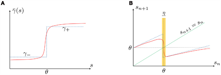
Figure A4. Effects of approximating the kinetic rate by a step function in the HHS model. (A) solid line – the original dashed line – the approximated step function (as in 4). (B) The map s_n+1 = g(s_n) near the threshold, in the intermittent mode: solid line – the original map [equation ((B.1))], dashed line – the map using the approximated step function for dotted line – the identity map s_n = s_n+1. Notice that in the original map g(s) changes gradually over the threshold in an area (rectangle of width η) that contain a single fixed point (in which s_n = s_n+1) while the approximated map has no fixed points. Also, the slopes of the original map are always smaller in magnitude than in the approximated map.