Local dynamics of a randomly pinned crack front: a numerical study

1. Introduction

The motion of a fracture front through a disordered medium is for obvious reasons of great practical importance. Nevertheless, it is a very complex problem which has kept material scientists and mechanical engineers occupied for almost two centuries [1]. In an attempt to simplify the problem, Schmittbuhl et al. [2] proposed to study the motion of a fracture front moving along a weak plane, thereby supressing the out of plane motion of the front. In a seminal experimental study, Schmittbuhl and Måløy [3] followed this idea up by sintering two sandblasted plexiglass plates together and then plying them apart from one edge. The sintering made the otherwise due to the sandblasting, opaque plates transparent. Where the plates were broken apart again, the opaqueness returned. Hence, it was possible to identify and follow the motion of the front since the plates would be transparent in front of the crack front and opaque behind it. There have been a large number of studies on this system following this initial work. Most of these studies have been theoretical or numerical in character and they have mostly dealt with the roughness of the crack front, see e.g., Ramanathan et al. [4], Delaplace et al. [5], Rosso and Krauth [6] Schmittbuhl et al. [7] and Santucci et al. [8]. See also the recent reviews by Bonamy [9] and Bonamy and Bouchaud [10].

The roughness is only one aspect of the motion of the crack front in this system. A first study of the dynamics of the front was published by Måløy and Schmittbuhl in 2001 [11]. The velocity distribution was measured and found to decay slower than an exponential. This was followed by a study by Måløy et al. [12] introducing the waiting time matrix technique making it possible to measure pixel by pixel the time the front sits still locally. This revealed an avalanche structure where portions of the front would sweep an area S with a velocity v before halting again. Both the distribution of areas and velocities were power laws. In two later papers, Tallakstad et al. [13] and Lengliné et al. [14], have continued and refined this work.

The fluctuating line model, based on the idea that the crack front moves as a pinned elastic line [2, 15], dominates the theoretical descriptions of the constrained crack problem. It is a top-down approach where the motion of the crack front is derived from continuum elastic theory. Its earliest use was to calculate the roughness exponent controlling the scaling properties of the crack front. If h(x, t) is the position of the crack front at time t and position x along its base line, then one finds the height-height correlation function 〈(h(x + Δx) − h(x))²〉 scaling as |Δx|^2ζ where ζ is the rougness exponent [2]. The most presise measurement of the roughness exponent withing the fluctuating line model to date is ζ = 0.388 ± 0.002 [6]. However, the experimental measurements of ζ gave systematically a much larger value, namely around 0.6—Schmittbuhl and Måløy [3] found ζ = 0.55 ± 0.05 and Delaplace et al. [5] ζ = 0.63 ± 0.03.

Santucci et al. [8] have reanalyzed data from a number of earlier studies, including Delaplace et al. [5], finding that the crack front has two scaling regimes: one small-scale regime described by a roughness exponent ζ₋ = 0.60 ± 0.05 and a large-scale regime described by a roughness exponent ζ₊ = 0.35 ± 0.05. Hence, there is a large scale roughness regime which is consistent with the fluctuating line model. However, the small scale regime is too rough.

Laurson et al. [16] has linked this regime to correlations in the pinning strength below the Larkin lenght within the fluctuating line model. This approach assumes that the physics behind both scaling regimes is describable within the same top-down model. Bonamy et al. [17] and Laurson et al. [16] have considered the crackling dynamics [18] of the fluctuating line model finding behavior consistent with the experimental measurements [11–14].

A very different approach to explain the roughness of the crack front has been proposed by Schmittbuhl et al. [7]. It is a bottom-up approach based on a stress-weighted gradient percolation process. This idea in turn has its origin in the proposal by Bouchaud et al. [19] that the crack front does not advance not only due to a competition between effective elastic forces and pinning forces at the front, but also by coalescence of damage in front of the crack with the advancing crack itself.

By refining the model proposed by Batrouni et al. [20] and Gjerden et al. [21], consisting of fibers clamped between a hard and a soft block and with a gradient in the breaking thresholds, we have identified two scaling regimes for the roughness of the advancing crack front [22]. On large scales we recover the roughness seen in the reanalysis of experimental data by Santucci et al. [8], ζ₊ = 0.39 ± 0.04, consistent with the fluctuating line model. On small scales, where the front advances mainly due to damage coalescence, we find the growth to be consistent with gradient percolation [23, 24]. As was shown by Hansen et al. [25], this implies a roughness exponent ζ₋ = 2/3. This value is consistent with the reanalysis of Santucci et al. [8].

We study in this paper the crackling dynamics in the fiber bundle model [20–22]. We find quantitative consistency with the experimental measurements. Hence, we demonstrate that this simple model contains the observed experimental features of constrained crack growth. It contains the essential physics of the problem. Since we have control over the crossover length scale between the crack advancing due to crack coalescence and due to pinning of the crack front as an elastic line, we analyse our results in light of this.

In Section 2, we describe the model in detail. Section 3.1 continues the analysis from Gjerden et al. [22] of the roughness of the crack front. In Gjerden et al. [22], we measured the roughness locally using the average wavelet coefficient method [26, 27]. Here we base our analysis on the variance of the front, again finding two regimes: a small-scale regime consistent with ordinary gradient percolation and a large-scale regime consistent with the fluctuating line model. In Section 3.2 we examine the velocity distribution during the motion of the crack front. Our data are consistent with the findings of Måløy et al. [12] and Tallakstad et al. [13]. Section 3.3 is devoted to an analysis of the geometry of the avalanches that occur during the motion of the crack front. The last section before the conclusion, Section 4 contains a tying up of loose ends through a discussion of the results.

The main aim of this paper has been to demonstrate that the simple model we use is capable of reproducing the experimental data. Hence, this simple fiber bundle model seems to contain the essential physics of the constrained crack problem.

2. Model and Method

The model we base our calculations on is a refinement of the fiber bundle model [28] used by Schmittbuhl et al. [7] and introduced by Batrouni et al. the year before [20]. We illustrate the model in Figure 1. L × L elastic fibers are placed in a square lattice between two parallel clamps. One of the clamps is infinitely stiff whereas the other has a finite Young modulus E and a Poisson ratio ν. All fibers are equally long and have the same elastic constant k.

FIGURE 1

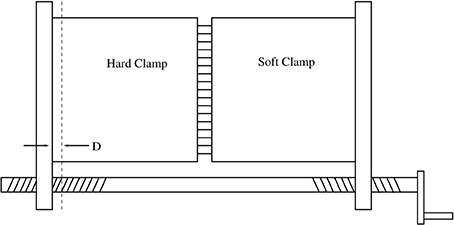
Figure 1. A contraption illustrating the fiber bundle model defined in Equations (1) and (2). When the handle is turned, the two clamps are moved away from each other. The distance over which they are moved is given by D. The hard clamp does not deform, whereas the soft clamp does.

We measure the position of the stiff clamp with respect to its position when all fibers carry zero force, D, see Figure 1. The force carried by the fiber at position (i, j), where i and j are coordinates in a cartesian coordinate system oriented along the two planes on which the fibers are clamped, is then

$\begin{array}{cc}{f}_{(i,j)}=-k(u_{(i,j)}-D),& (1)\end{array}$

where u_(i,j) is the elongation of the fiber at (i, j).

The fibers redistribute the forces they carry through the response of the soft clamp. The redistribution of forces is accomplished by using the Green function connecting the force f_(m,n) acting on the clamp from fiber (m, n) with the deformation u_(i,j) at fiber (i, j), [29]

$\begin{array}{cc}{u}_{(i,j)}={\displaystyle \sum _{(m,n)}{G}_{(i,j),(m,n)}}{f}_{(m,n)},& (2\text{a})\end{array}$

$\begin{array}{cc}\begin{array}{l}{G}_{(i,j),(m,n)}=\hfill \\ \frac{1-{\nu }^2}{\pi E{a}^2}{\displaystyle {\int }_{-a/2}^{a/2}d}x{\displaystyle {\int }_{-a/2}^{a/2}d}y\frac{1}{|{\overrightarrow{r}}_{(i,j)}-{\overrightarrow{r}}_{(m+x,n+y)}|}.\end{array}& (2\text{b})\end{array}$

where a is the distance between neighboring fibers. The integration in Equation (2b) is performed over the Voronoi cell around each fiber. $\overrightarrow{r}$_(i,j) is the position of fiber (i, j). $\overrightarrow{r}$_{(m+x, n+y)} is the position of a point (x, y) in the Voronoi cell surrounding the fiber at (m, n).

The equation set, Equations (2) and (2b), is solved using a Fourier accelerated conjugate gradient method [30, 31].

The Green function, Equation (2b), is proportional to (Ea)⁻¹. The elastic constant of the fibers, k, must be proportional to a². The linear size of the system is aL. Hence, by changing the linear size of the system without changing the discretization a, we change L → λL but leave (Ea) and k unchanged. If we on the other hand change the discretization without changing the linear size of the system, we simultaneously set L → λL, (Ea) → λ (Ea) and k → k/λ². Based on these observations, we define a scaled Young modulus

$\begin{array}{cc}e=\frac{Ea}{L}.& (3)\end{array}$

Hence, changing e without changing k is equivalent to changing L—and hence the linear size of the system—while keeping the elastic properties of the system constant [32]. This is a central point in what follows.

The fibers are broken by using the quasistatic approach [33]. That is, we assign to each fiber (i, j) a threshold value t_(i,j). They are then broken one by one by identifying the fiber which satisfies max_(i,j) (f_(i,j)/t_(i,j)) when the forces f_i,j have been calculated for D = 1. This ratio is then equal to 1/D where D is the value at which the fiber fails.

In the constrained crack growth experiments of Schmittbuhl and Måløy [3], the two sintered plexiglass plates were plied apart from one edge. In the numerical modeling of Schmittbuhl et al. [7], an asymmetric loading was accomplished by introducing a linear gradient in D. Rather than implementing an asymmetric loading, we use here a gradient in the threshold distribution, t_(i,j) = gj + r_(i,j), where g is the gradient and r_(i,j) is a random number drawn from a flat distribution on the unit interval.

In order to follow the crack front as the breakdown process develops, we implement the “conveyor belt” technique [21, 34]. We illustrate this technique in Figure 2. Fiber bundle forms a rectangle of width L and length nL, where n > 1. However, we do not consider all fibers at once, but a square of size L × L. This is the red square in the figure. The square is initially placed at the bottom of the L × nL strip and at regular intervals, the bottom row in the square is removed and a new intact row is added at the top. In this way, the square moves along the strip, eventually passing from the bottom to the top. The speed at which the square moves is adjusted so that the crack front, shown as a black rough curve in the figure, stays roughly in the middle of the red square.

FIGURE 2

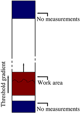
Figure 2. The system we consider is a strip of width L and length nL. We calculate the force distribution within the red square. This has size L × L. At the beginning of the calculation, the lower edge of the red square coincides with the lower edge of the strip. As the calculation proceeds, the lower row contaning only failed fibers is removed from the red square and a row on intact fibers is added at the top row. Hence, the red square moves along the strip. The speed at which it moves is adjusted so that the crack front remains roughly in the middle of the red square. When the red square overlaps with the blue regions of length L/2 (bottom) and 3L/4 (top), no measurements are made of the crack front.

Only after the square has passed the L/2 first rows (marked in blue in Figure 2) do we record the position of the front. This is to ensure that the front has entered a steady-state regime. We also do not record whence the red square is at a distance 3L/4 from the top. This is indicated as the blue region at the top of the figure. This is done to avoid boundary effects at this edge.

3. Results

3.1. Roughness and Dynamical Scaling

In Gjerden et al. [22], we presented evidence for two scaling regimes in the model we study here. For small values of the scaled elastic constant e—or equivalently large length scales—we found a roughness exponent ζ₊ = 0.39 ± 0.04, which is consistent with the flucutating line model. On small scale, we found that the roughness exponent ζ₋ was consistent with the value 2/3, the value expected in gradient percolation [25]. However, at these small scales, the fracture is fractal and we determined its fractal dimension to be 1.77 ± 0.02, which is consistent with that of the percolation hull, 7/4 [24].

We note in this connection that in the limit of completely stiff clamps, the system becomes equivalent to gradient percolation [23, 24]. Our statement on the small scale behavior of the soft clamp fiber bundle model is then that it is in the percolation universality class even though the clamps are not stiff.

In this section, we present further results concerning the existence of two scaling regimes in the soft clamp fiber bundle model beyond those that were presented in Gjerden et al. [22].

We identify the crack front by first eliminating all islands of surviving fibers behind it and all islands of failed fibers in front of it. We measure “time” n in terms of the number of failed fibers. After an initial period, the system settles into a steady state. We then record the position of the crack front j = j(i, n = 0) after having set n = 0. We then define the position at later times n > 0 relative to this initial position,

$\begin{array}{cc}{h}_i(n)=j(i,n)-j(i,n=0).& (4)\end{array}$

This is the same definition as was used by Schmittbuhl and Måløy in their experimental studies [3]. The front as it has now been defined will contain overhangs. That is, there may be multiple values of h_i(n) for the same i and n values. We only keep the largest h_i(n), i.e., we implement the Solid-on-Solid (SOS) front.

We define the average position of the front as

$\begin{array}{cc}\langle h(n)\rangle =\frac{1}{L}{\displaystyle \sum _{i=1}^L{h}_i}(n),& (5)\end{array}$

and the front width as

$\begin{array}{cc}w{(n)}^2=\frac{1}{L}{\displaystyle \sum _{i=1}^L(h_i(}n)-\langle h(n)\rangle {)}^2.& (6)\end{array}$

We assume that 〈h〉 grows linearly with the number of broken fibers n, 〈h〉 ∝ n. In the following, we measure time in terms of 〈h〉 rather than n.

3.1.1. Small scales

We now set e = 3.1. This places us in the regime that was identified in Gjerden et al. [22] as the small scale one. Here the fracture front has the fractal properties of the percolation hull. In Gjerden et al. [22], we used the averaged wavelet coefficient method to measure ζ₋. In Figure 3, we show the width w, defined in Equation (6) as a function of 〈h〉. When w is rescaled as w/g^α₋ and 〈h〉 as 〈h〉/g^β₋, we find data collapse for different values of the threshold gradient g. Hence, we have

$\begin{array}{cc}w(\langle h\rangle ,g)=g^{{\alpha }_{-}}{\omega }_{-}\left(\frac{\langle h\rangle }{g^{{\beta }_{-}}}\right),& (7)\end{array}$

where ω₋ is a scaling function given by

$\begin{array}{cc}{\omega }_{-}(q)=\{\begin{array}{ll}{q}^{{\delta }_{-}}\hfill & \text{if}q\to 0,\hfill \\ constant\hfill & \text{if}q\to \infty .\hfill \end{array}& (8)\end{array}$

FIGURE 3

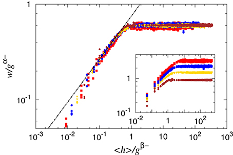
Figure 3. One-parameter scaling of the SD of the width of the front as a function of the average position of the front as the front moves forward from some initial (rough) configuration. The main figure shows data collapse for α₋ = β₋ = 4/7, and the inset shows the same data without rescaling. The straight line has slope 288/637 ≈ 0.45—see text. The data are extracted from simulations with, from top-down in the inset, g ∈ (0.05, 0.1, 0.2, 0.5). Each data set is based on 100 samples for L = 64 and n = 5, 10 samples for L = 128 and n = 5, and 10 samples for L = 256 and n = 2.

Hence, the front width saturates as 〈h〉 grows beyond a given scale. Furthermore, we assume that w~ 〈h〉^δ₋ for 〈h〉 much smaller than this scale. We will determine δ₋ in a moment. Assuming the percolation universality class on small scales, we expect the two scaling exponents α and β to obey the relation α₋ = β₋ = ν(1 + ν) = 4/7, where ν = 4/3, the percolation value. The derivation of the relations between α₋, β₋ and ν is given in Hansen et al. [25].

We now derive the value of δ₋ by relating 〈h〉 to the number of fibers below and including the front, A, by the fractal dimension D_A = 91/48 [35], 〈h〉^D_A ~ A. Invoking Mandelbrot's area-perimeter relation, we may also relate the length of the front, l to the number of fibers below and including the front, l ~ A^D_h/2, where D_h = 7/4 [24, 37]. Eliminating A between these two expressions leads to l ~ 〈h〉^D_HD_A/2. We relate the length of the front l to its width w by the relation l ~ w^D_H(L/w) [22]. Eliminating l between these two relations gives

$\begin{array}{cc}w~{\langle h\rangle }^{{\delta }_{-}}={\langle h\rangle }^{D_A{D}_H/(2D_H-2)}={\langle h\rangle }^{288/637}.& (9)\end{array}$

Hence, we have that

$\begin{array}{cc}{\delta }_{-}=\frac{288}{637}\approx \mathrm{0.45.}& (10)\end{array}$

The straight line in Figure 3 has this slope.

By invoking Family-Vicsek scaling [36], a dynamical exponent κ₋ may be defined. By setting W to be the width of the system in the x direction, i.e., orthogonally to the direction of the gradient, Family-Vicsek scaling takes the form

$\begin{array}{cc}w(W,\langle h\rangle )=W^{{\zeta }_{-}}{f}_{-}\left(\frac{\langle h\rangle }{W^{{\kappa }_{-}}}\right),& (11)\end{array}$

where

$\begin{array}{cc}{f}_{-}(q)=\{\begin{array}{ll}{q}^{{\zeta }_{-}/{\kappa }_{-}}\hfill & \text{if}q\to 0,\hfill \\ constant\hfill & \text{if}q\to \infty .\hfill \end{array}& (12)\end{array}$

We are here keeping the gradient g constant. Since the behavior of the Family-vicsek scaling function f must be the same as the one defined in Equation (8), we find the relation

$\begin{array}{cc}\frac{{\zeta }_{-}}{{\kappa }_{-}}={\delta }_{-},& (13)\end{array}$

leading to

$\begin{array}{cc}{\kappa }_{-}=\frac{637}{432}\approx \mathrm{1.47.}& (14)\end{array}$

3.1.2. Large scales

Figure 4 shows the corresponding one-parameter scaling as in Figure 3, but now for systems with a much lower e = 7.8 × 10⁻⁴, placing us in the realm of the fluctuating line model [22]. We define as for the small scale study scaling relations Equations (7), (8), (11), and (12) corresponding relation, but where “−” has been exchanged for “+.”

FIGURE 4

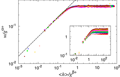
Figure 4. One-parameter scaling of w as a function of 〈h〉 with g as the scaling parameter. The main figure shows data collapse for α₊ = β₊ = 0.4. The inset shows unscaled data. The slope of the straight line is 0.52. The parameter values are, from top-down in the inset, g ∈ (0.007, 0.008, 0.01, 0.015, 0.02, 0.03). The data sets are based on 200–800 samples for L = 64 and n = 10.

The two scaling exponents that produce data collapse are α₊ = β₊ = 0.4. By a least squares fit, we determine

$\begin{array}{cc}w~{\langle h\rangle }^{{\delta }_{+}}={\langle h\rangle }^{0.52\pm 0.05}.& (15)\end{array}$

This value is very close to the one seen for large e values, and consistent with the experimental measurement of Tallakstad et al. [13], who found 0.55 and Schmittbuhl et al. [38] who found 0.52.

By invoking Family-Vicsek scaling as for the small-scale case, we may determine the dynamical exponent

$\begin{array}{cc}\frac{{\zeta }_{+}}{{\kappa }_{+}}={\delta }_{+},& (16)\end{array}$

so that κ₊ = 0.75 ± 0.07. This is consistent with the value reported by Duemmer and Krauth for the fluctuating line model, κ = 0.770 ± 0.005 [39].

The dynamical exponent reported by Måløy and Schmittbuhl [11] for the PMMA system was κ = 1.2. This value sits between the values we find for κ₋ and κ₊.

3.1.3. Height fluctuations

It was observed by Santucci et al. [8] that the large-scale roughness regime shows a gaussian distribution of the height fluctuations, whereas in the small-scale it broadens to a non-gaussian distribution, see Figure 3 in Santucci et al. We investigate this in our model. We define the height fluctuations as Δh(1) = |h_{i + 1}(n) − h_i(n)|. By changing the elastic constant, L in our model while keeping the step size constant, the result is equivalent to changing the step size in the experiment, where they measured |h(x + δ) − h(x)| for different values of δ. We show in Figure 5 the distribution of fluctuations for different elastic constant E. We observe that for soft systems, the distribution is gaussian (i.e., follows a parabola in the plot). As the system stiffens, the distribution broadens.

FIGURE 5

Figure 5. Histogram of height fluctuations with respect to Δh(1) = |h_{i + 1}(n) − h_i(n)| for different elastic constants. The distribution follows a gaussian when the system is soft and broadens when the system stiffens. This is equivalent to changing the step size between measurements of the crack front, as was done in Santucci et al. [8]. These measurements are based on a single strip of with L = 128, and length nL = 10 × 128. The data were recorded when the front was at 112 different positions, spaced so far apart that they were statistically independent.

3.2. Local Velocity Distribution

We examine the distribution of local velocities using the Waiting Time Matrix (WTM) method [12]. The WTM method consists of letting the fracture move across a matrix with all elements initially equal to zero in discrete time steps. At every time step, the matrix elements containing the front are incremented by one. When the front has passed, the matrix contains the time the front spent in each position measured in time steps. Hence, matrix elements contaning low values correspond to rapid front movements and large values correspond to slow, pinned movement. One may then calculate the spatiotemporal map of velocities, v(x, y), by inverting the waiting time recorded in each matrix element. From this map we then calculate the global average velocity 〈v〉 and the distribution of local velocities P(v). Tallakstad et al. find experimentally that this distribution follows a power law,

$\begin{array}{cc}P(v/\langle v\rangle )~{(v/\langle v\rangle )}^{-\eta },\text{for}v/\langle v\rangle >1,& (17)\end{array}$

with the exponent η = 2.55 ± 0.15 [12, 13].

The results from our simulations are shown in Figure 6 for scaled elastic constant e = 1.6 × 10⁻⁴ and 7.8 × 10⁻⁴, which places us in the large-scale regime. We use these values for e throughout this section unless explicitly stated otherwise. The slope in the figure is obtained through a linear fit and has the value η₊ = 2.53, where the subscript “+” indicates that this is in the large-scale regime.

FIGURE 6

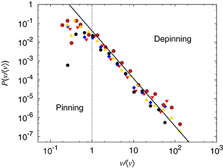
Figure 6. Distribution of local velocities scaled by the global average velocity. Results are based on simulations of sizes L = 64, 128 with e = 1.56 × 10⁻⁴, 7.81 × 10⁻⁴, respectively, and loading gradient in the range g ∈ [0.01 − 0.05]. A fit to the data for v > 〈v〉 yields a power law behavior with an exponent of −2.53. The values of e correspond to the fluctuating line regime.

The data in this section is based on systems of width L = 64 and length nL = 5 × 64 or L = 128 and nL = 2 × 128. The waiting time matrix was calculateed from 15460 (L = 64) or 12288 (L = 128) snapshots of the front position.

3.2.1. Space and time correlations

From the local velocities, still in the large-scale regime, we calculate the normalized correlation functions in space, G(Δx), and time, G(Δt)

$\begin{array}{cc}G(\Delta x)={\langle \frac{\langle [v(x+\Delta x,t)-{\langle v\rangle }_x][v(x,t)-{\langle v\rangle }_x]\rangle }{{\sigma }_x^2}\rangle }_t,& (18\text{a})\end{array}$

$\begin{array}{cc}G(\Delta t)={\langle \frac{\langle [v(x,t+\Delta t)-{\langle v\rangle }_t][v(x,t)-{\langle v\rangle }_t]\rangle }{{\sigma }_t^2}\rangle }_x.& (18\text{b})\end{array}$

σ_x/t and 〈 〉_x/t denote standard deviation and average over x or t.

The results for G(Δx) are presented in Figure 7, where we fit the data to the function

$\begin{array}{cc}G(\Delta x)=A{\left(\frac{\Delta x}{x^{*}}\right)}^{-{\tau }_x}\exp \left(-\frac{\Delta x}{x^{*}}\right),& (19)\end{array}$

where x* = 0.1L and τ_x = 0.4. This functional form was proposed by Tallakstad et al. [13] with τ_x = 0.53 ± 0.12. We note that the cutoff in our data is much sharper than the proposed functional form. This may be due to the small system sizes that are available numerically.

FIGURE 7

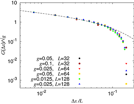
Figure 7. Spatial correlation function G(Δx). Data collapse is obtained when Δx is scaled with the system size and G(Δx) is scaled with $\sqrt{g}$. The line is a fit to a power law with exponential cutoff G(Δx) = A(Δx/L)^−0.4exp(− Δx/0.1L). The system sizes and elastic constant used are as in Figure 6.

In Figure 8, we show the results of the analysis of the temporal velocity distribution. Again, we attempt to fit the data to a power law with exponential cutoff,

$\begin{array}{cc}G(\Delta t)=B{\left(\frac{\Delta t}{t^{*}}\right)}^{-{\tau }_t}\exp \left(-\frac{\Delta t}{t^{*}}\right),& (20)\end{array}$

with t* = 0.25/〈v〉 and exponent τ_t = 0.43. This functional form was proposed by Tallakstad et al. [13], including the value τ_t = 0.43.

FIGURE 8

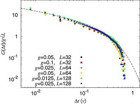
Figure 8. Temporal correlation function D(Δt). Best data collapse is obtained when scaling Δt by 1/〈v〉 and G(Δt) by 〈v〉^0.43g$\sqrt{L}$. The line is a fit to a power law with exponential cutoff G(Δt) = B(Δt〈v〉)^−0.43 exp(− Δt〈v〉/0.25). The system sizes and elastic constant used are as in Figure 6.

We note that the prefactor A in Equation (19) is, according to Figure 7, proportional to $\sqrt{g}$, where g is the gradient in the threshold distribution. Likewise, the prefactor B in Equation (20) is, according to Figure 5, proportional to g$\sqrt{L}$.

3.3. Cluster Analysis

In the following we analyze the geometrical structure of the areas swept by the crack front during avalanches. We denote such an area a cluster. Also here we use values of e.

Tallakstad et al. [13] define a pinning regime where v < 〈v〉 and a depinning regime where v > 〈v〉. As they did, we construct thresholded velocity maps V_C in such a way that

$\begin{array}{cc}{V}_C=\{\begin{array}{ll}1,\hfill & \text{for }v\ge C\langle v\rangle \hfill \\ 0,\hfill & \text{for }v<C\langle v\rangle \hfill \end{array},& (21)\end{array}$

in the depinning regime and

$\begin{array}{cc}{V}_C=\{\begin{array}{ll}1,\hfill & \text{for }v\le \langle v\rangle /C\hfill \\ 0,\hfill & \text{for }v>\langle v\rangle /C\hfill \end{array},& (22)\end{array}$

in the pinning regime. C is a constant in the range of 2–12 for depinning and 1.5−6 for pinning for our simulations. For larger system sizes, larger C are possible. Examples of these matrices are shown in Figure 9, where the structural difference between depinning and pinning clusters can be seen. In the spirit of de Saint-Exupéry we may characterize the pinning clusters as “snakelike,” whereas the depinning clusters are “elephant-in-snakelike” [40]. The following analysis uses only L = 64 and L = 128, and are based on 250 and 100 samples, respectively. g = 0.025 for the smaller systems, and g = 0.0125 for the larger systems. For L = 64, e = 1.6 × 10⁻⁴, and for L = 128, e = 7.8 × 10⁻⁴. The systems will for these e-values behave virtually identical [22].

FIGURE 9

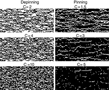
Figure 9. Part of the thresholded velocity matrix showing depinning clusters on the left and pinning clusters on the right. The images are from a system of size L = 128, g = 0.0125, and e = 7.8 × 10⁻⁴. White areas are areas where the local velocities are either above C〈v〉 (depinning) or below $\frac{1}{\text{C}}$〈v〉 (pinning). With the value of the e that has been used, we are in the fluctuating line regime. Hence, the pinning is localized at the crack front.

3.3.1. Size distribution of clusters

We denote the number of fibers in a cluster the area of the cluster S. Both experiments [12, 13] and numerical simulations using the fluctuating line model [17] on in-plane fracture, show a power law distribution P(S) ~ S^−γ for S with exponent close to γ = 1.56 [13] or γ = 1.65 [17].

We show in Figure 10 the probability distribution of S both for pinning and depinning for scaled elastic constant e = 1.6 × 10⁻⁴. Our data is consistent with previous measurements, but due to the limited size of the numerical simulations currently available, the exponent cannot be accurately determined. One prominent feature of the clusters is that due to the small system size, the presence of large clusters for low values of C suppresses the number of smaller clusters, and for high values of C, the number of large clusters is reduced by the filtering process in C. This is a pure finite size effect. The experiments, which would correspond to a very large simulation size, shows no such dependence on C. A direct comparison between the experimental and our data is given in Figure 11.

FIGURE 10

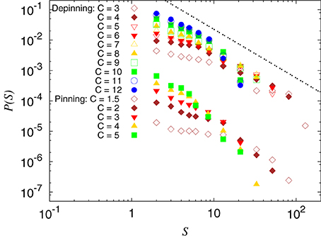
Figure 10. Probability distribution function of the size of clusters, S, for a range of C values for both pinning (lower cluster of points) and depinning clusters (upper cluster of points). The data for pinning clusters are shifted down by 0.005 to visually separate the two regimes. The slope of the line is γ = 1.6. L = 64, and e = 1.6 × 10⁻⁴.

FIGURE 11

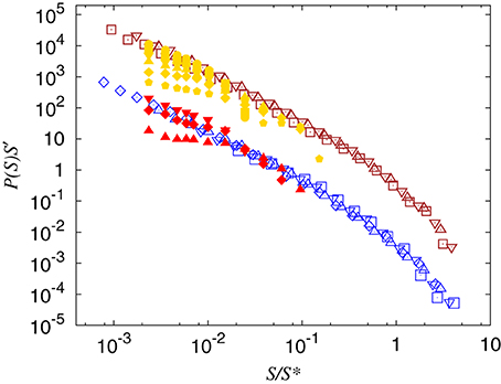
Figure 11. Size distribution of clusters. Depinning clusters on top and pinning clusters below. The longest data series (unfilled markers) are experimental data obtained with permission from the authors [13]. The shorter data series (filled markers) are numerical data from Figure 10. The experimental data are unchanged from Tallakstad et al. [13], so S′ = S*^γ and S* are as given in Tallakstad et al. [13]. Due to lack of direct physical parameter comparison, the numerical data are scaled to match the experimental data to verify similar behavior.

3.3.2. Aspect ratio of clusters

Next, we extract the linear extensions of the clusters in the growth direction and orthogonally to it. This is done by enclosing each cluster in a bounding box of size l_x by l_y. Although the appearance differs greatly between pinning and depinning clusters, the method for determining l_x and l_y are the same.

We now turn to examinining the relation between l_y and l_x. We plot these against each other in Figure 12. This data is more well-behaved than the probability distributions, so scaling relations are more pronounced. The data are consistent with a relation of type

$\begin{array}{cc}{l}_y~l_x^H,& (23)\end{array}$

as studied both by Tallakstad et al. [13] and Bonamy et al. [17] in, respectively, the experimental system and numerically using the fluctuating line model.

FIGURE 12

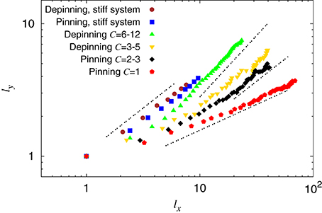
Figure 12. Local scaling of the clusters. The lines are guides to the eye, but the slopes are based on linear regression and the values are in descending order 0.91, 0.67, 0.67, and 0.39. The data labeled stiff system are from simulations using a Young's modulus four orders of magnitude greater than what is used in the rest of the simulations. L = 128, g = 0.0125, and e = 7.8 × 10⁻⁴ and e = 7.8.

We see a clear dependency of H on parameters such as e and C. Considering the depinning case first for e = 7.8 × 10⁻⁴, we divide the data between C^high ∈ [6 − 12], a group containing data from only the highest local velocities, and C^low ∈ [3 − 5], containing lower local velocities. There is a clear visual difference in behavior between the two groups: The group with the higher C values, have the higher slope. We measure the corresponding exponents to be H^high_d = 0.9 and H^low_d = 0.65.

In the pinning regime we similarly divide between low and high local velocity effects, except that the range of available C is much smaller, so we find C^high = 2, 3 and C^low = 1. This yields the two exponents H^high_p = 0.65 and H^low_p = 0.4.

It has been suggested that H is another measure of the roughness exponent defined in Equation (11), ζ [12, 16, 17]. In order to test this, we have added data both for pinning and depinning of a stiff system (e = 7.8) in Figure 12. If the conjecture is right in this case, we would expect a H exponent equal to 2/3. We have added such slopes, and the result is consistent with this conjecture.

Another way to examine these scaling relations is to check the relation between l_x, l_y and S. We expect to see a power law relationship of type

$\begin{array}{cc}{l}_i~S^{{\alpha }_i},& (24)\end{array}$

since the size of the clusters are related through power laws. The data are plotted in Figure 13, in which data for the highest local velocities are not included, C = C^low for both pinning and depinning. In the depinning regime, we find the exponents α^d_x = 0.6 and α^d_y = 0.4. Eliminating S, we get a measure of H through

$\begin{array}{cc}{l}_y~l_x^{{\alpha }_y/{\alpha }_x}=l_x^H,& (25)\end{array}$

resulting in H_d = 0.65. In the pinning regime we find α^p_x = 0.75 and α^p_y = 0.3, yielding H_p = 0.4.

FIGURE 13

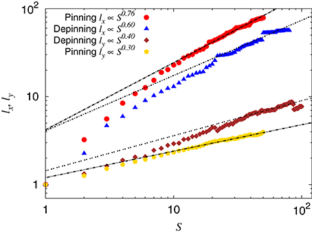
Figure 13. Linear size of both pinning and depinning clusters as a function of cluster size. The simulation parameters are the same as for Figure 12.

These results are to be compared to the experimental measurements of Tallakstad et al. [13] giving α_x = 0.62 ± 0.04 in pinning and the depinning regime and α_y = 0.41 ± 0.06 or 0.34 ± 0.05 in the depinning regime depending on how the bounding box was defined. This leads to the value H = α_y/α_x = 0.66 or 0.55 depending on the bounding box used. Bonamy et al. [17] found H = 0.65 ± 0.05 numerically using the fluctuating line model.

4. Discussion and Conclusion

We have studied the fracture front in the soft clamp fiber bundle model when a gradient in the threshold distribution is introduced. The rescaled elastic constant e and the threshold gradient g are the most important input parameters in the model. g effectively controls the loading conditions and mimicks the plying apart of the two sintered PMMA plates in the experiment of Tallakstad et al. [13]. A high value for g amounts to a large angle of contact between the materials, or slow loading conditions, and vice versa. As long as 1/g is in a range where it allows the front to develop but not extend out of the system, we see no change in any scaling exponents we have investigated when g is changed. This behavior echoes the experimental study where no dependence on the loading conditions was found and the average propagation velocity of the front spanned more than four and a half orders of magnitude [13].

The parameter e, defined in Equation (3), controls the material behavior. A small value for e may model a system of low modulus of elasticity, but also a system at long length scales. Likewise, a large e may model a system of large elastic modulus, but also a system at small length scales. We have in this paper associated the different e values we have studied with the scales at which we study the system.

A number of scaling exponents have been measured and compared to their experimental counterparts. We summarize the most important in Table 1.

TABLE 1

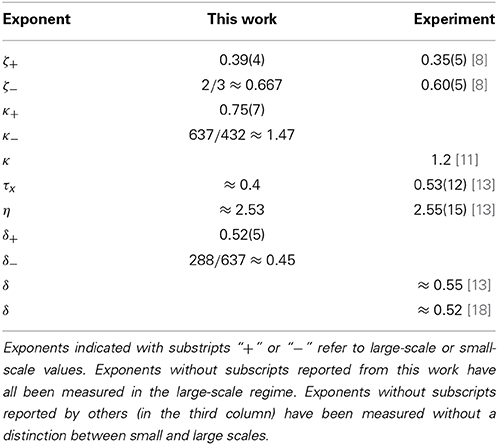
Table 1. Comparison between the exponents measured in the work and those found experimentally.

In Section 3.3.2 we discussed shape of the clusters defined through the avalanches. The following pucture emerges: For low values of e, the fracture process is due to stress concentration leading to damage forming on the fracture front. This regime is classified by a roughness exponent of ζ₊ = 0.39 ± 0.04. By studying the shape of the clusters defined through the avalanche dynamics, we find the same value for H. As e increases—corresponding to decreasing the length scale at which the system is observed—the clusters formed by the avalanche process changes shape and are now characterized by an exponent H = ζ₋ = 0.67, while the fracture front itself is still characterized by ζ₊. As e is increased further, damage begins to form ahead of the front, and the front now grows due to damage coalescence. At this point, the roughness exponent changes from 0.39 and grows into 0.67. At higher e, both the burst process and the roughness of the front is now characterized by the larger exponent H = ζ₋ = 0.67.

Conflict of Interest Statement

The authors declare that the research was conducted in the absence of any commercial or financial relationships that could be construed as a potential conflict of interest.

Acknowledgments

We are grateful for discussions and suggestions by D. Bonamy, K. J. Måløy, L. Ponson, J. Schmittbuhl, and K. T. Tallakstad. This work was supported by the Norwegian Research Council (NFR) under grant number 177591/V30. Part of this work made use of the facilities of HECToR, the UK's national high performance computing service, which is provided by UoE HPCx Ltd at the University of Edinburgh, Cray Inc and NAG Ltd, and funded by the Office of Science and Technology through EPSRC's High End Computing Programme.

References

1. Lawn BR. Fracture of Brittle Solids, 2nd Edn. Cambridge: Cambridge University Press (1993). doi: 10.1017/CBO9780511623127

CrossRef Full Text | Google Scholar

2. Schmittbuhl J, Roux S, Vilotte JP, Måløy KJ. Interfacial crack pinning: effect of nonlocal interactions. Phys Rev Lett. (1995) 74:1787. doi: 10.1103/PhysRevLett.74.1787

Pubmed Abstract | Pubmed Full Text | CrossRef Full Text | Google Scholar

3. Schmittbuhl J, Måløy KJ. Direct observation of a self-affine crack propagation. Phys Rev Lett. (1997) 78:3888. doi: 10.1103/PhysRevLett.78.3888

CrossRef Full Text | Google Scholar

4. Ramanathan S, Ertas D, Fisher DS. Quasistatic crack propagation in heterogeneous media. Phys Rev Lett. (1997) 79:873. doi: 10.1103/PhysRevLett.79.873

CrossRef Full Text | Google Scholar

5. Delaplace A, Schmittbuhl J, Måløy KJ. High resolution description of a crack front in a heterogeneous Plexiglas block. Phys Rev E (1999) 60:1337. doi: 10.1103/PhysRevE.60.1337

Pubmed Abstract | Pubmed Full Text | CrossRef Full Text | Google Scholar

6. Rosso A, Krauth W. Roughness at the depinning threshold for a long-range elastic string. Phys Rev E (2002) 65:025101(R). doi: 10.1103/PhysRevE.65.025101

Pubmed Abstract | Pubmed Full Text | CrossRef Full Text | Google Scholar

7. Schmittbuhl J, Hansen A, Batrouni GG. Roughness of interfacial crack fronts: stress-weighted percolation in the damage zone. Phys Rev Lett. (2003) 90:045505. doi: 10.1103/PhysRevLett.90.045505

Pubmed Abstract | Pubmed Full Text | CrossRef Full Text | Google Scholar

8. Santucci S, Grob M, Toussaint R, Schmittbuhl J, Hansen A, Måløy KJ. Fracture roughness scaling: a case study on planar cracks. Europhys Lett. (2010) 92:44001. doi: 10.1209/0295-5075/92/44001

CrossRef Full Text | Google Scholar

9. Bonamy D. Intermittency and roughening in the failure of brittle heterogeneous materials. J Appl Phys D (2009) 42:214014. doi: 10.1088/0022-3727/42/21/214014

CrossRef Full Text | Google Scholar

10. Bonamy D, Bouchaud E. Failure of heterogeneous materials: a dynamic phase transition? Phys Rep. (2011) 498:1–44. doi: 10.1016/j.physrep.2010.07.006

Pubmed Abstract | Pubmed Full Text | CrossRef Full Text | Google Scholar

11. Måløy KJ, Schmittbuhl J. Dynamical events during slow crack propagation. Phys Rev Lett. (2001) 87:105502. doi: 10.1103/PhysRevLett.87.105502

Pubmed Abstract | Pubmed Full Text | CrossRef Full Text | Google Scholar

12. Måløy KJ, Santucci S, Schmittbuhl J, Toussaint R. Local waiting time fluctuations along a randomly pinned crack front. Phys Rev Lett. (2006) 96:045501. doi: 10.1103/PhysRevLett.96.045501

Pubmed Abstract | Pubmed Full Text | CrossRef Full Text | Google Scholar

13. Tallakstad KT, Toussaint R, Santucci S, Schmittbuhl J, Måløy KJ. Local dynamics of a randomly pinned crack front during creep and forced propagation: an experimental study. Phys Rev E (2011) 83:046108. doi: 10.1103/PhysRevE.83.046108

Pubmed Abstract | Pubmed Full Text | CrossRef Full Text | Google Scholar

14. Lengliné O, Toussaint R, Schmittbuhl JE. Ampuero JP, Tallakstad KT. Santucci S, et al. Average crack-front velocity during subcritical fracture propagation in a heterogeneous medium. Phys Rev E (2011) 84:036104. doi: 10.1103/PhysRevE.84.036104

Pubmed Abstract | Pubmed Full Text | CrossRef Full Text | Google Scholar

15. Bouchaud JP, Bouchaud E, Lapasset G, Planès J. Models of fractal cracks. Phys Rev Lett. (1993) 71:2240. doi: 10.1103/PhysRevLett.71.2240

Pubmed Abstract | Pubmed Full Text | CrossRef Full Text | Google Scholar

16. Laurson L, Santucci S, Zapperi S. Avalanches and clusters in planar crack front propagation. Phys Rev E (2010) 81:046116. doi: 10.1103/PhysRevE.81.046116

Pubmed Abstract | Pubmed Full Text | CrossRef Full Text | Google Scholar

17. Bonamy D, Santucci S, Ponson L. Crackling dynamics in material failure as the signature of a self-organized dynamic phase transition. Phys Rev Lett. (2008) 101:045501. doi: 10.1103/PhysRevLett.101.045501

Pubmed Abstract | Pubmed Full Text | CrossRef Full Text | Google Scholar

18. Sethna J, Dahmen K, Myers C. Crackling noise. Nature (2001) 410:242–250. doi: 10.1038/35065675

Pubmed Abstract | Pubmed Full Text | CrossRef Full Text | Google Scholar

19. Bouchaud E, Bouchaud JP, Fisher DS, Ramanathan S, Rice JR. Can crack front waves explain the roughness of cracks? J Mech Phys Sol. (2002) 50:1703. doi: 10.1016/S0022-5096(01)00137-5

CrossRef Full Text | Google Scholar

20. Batrouni GG, Hansen A, Schmittbuhl J. Heterogeneous interfacial failure between two elastic blocks. Phys Rev E (2002) 65:036126. doi: 10.1103/PhysRevE.65.036126

Pubmed Abstract | Pubmed Full Text | CrossRef Full Text | Google Scholar

21. Gjerden KS, Stormo A, Hansen A. A model for stable interfacial crack growth. J Phys Conf Series (2012) 402:012039. doi: 10.1088/1742-6596/402/1/012039

Pubmed Abstract | Pubmed Full Text | CrossRef Full Text | Google Scholar

22. Gjerden KS, Stormo A, Hansen A. Universality classes in constrained crack growth. Phys Rev Lett. (2013) 111:135502. doi: 10.1103/PhysRevLett.111.135502

Pubmed Abstract | Pubmed Full Text | CrossRef Full Text | Google Scholar

23. Sapoval B, Rosso M, Gouyet JF. The fractal nature of a diffusion front and the relation to percolation. J Phys Lett. (1985) 46:149–156. doi: 10.1051/jphyslet:01985004604014900

CrossRef Full Text | Google Scholar

24. Gouyet JF, Rosso M. Diffusion fronts and gradient percolation: a survey. Physica A (2005) 357:86–96. doi: 10.1016/j.physa.2005.05.054

Pubmed Abstract | Pubmed Full Text | CrossRef Full Text | Google Scholar

25. Hansen A, Batrouni GG, Ramstad T, Schmittbuhl J. Self-affinity in the gradient percolation problem. Phys Rev E (2007) 75:030102. doi: 10.1103/PhysRevE.75.030102

Pubmed Abstract | Pubmed Full Text | CrossRef Full Text | Google Scholar

26. Mehrabi AR, Rassamdana H, Sahimi M. Characterization of long-range correlations in complex distributions and profiles. Phys Rev E (1997) 56:712. doi: 10.1103/PhysRevE.56.712

CrossRef Full Text | Google Scholar

27. Simonsen I, Hansen A, Nes OM. Determination of the Hurst exponent by use of wavelet transforms. Phys Rev E (1998) 58:2779. doi: 10.1103/PhysRevE.58.2779

CrossRef Full Text | Google Scholar

28. Pradhan S, Hansen A, Chakrabarti BK. Failure processes in elastic fiber bundles. Rev Mod Phys. (2010) 82:499. doi: 10.1103/RevModPhys.82.499

Pubmed Abstract | Pubmed Full Text | CrossRef Full Text | Google Scholar

29. Johnson KL. Contact Mechanics. Cambridge: Cambridge University Press (1985). doi: 10.1017/CBO9781139171731

CrossRef Full Text | Google Scholar

30. Batrouni GG, Hansen A, Nelkin M. Fourier acceleration of relaxation processes in disordered systems. Phys Rev Lett. (1986) 57:1336. doi: 10.1103/PhysRevLett.57.1336

Pubmed Abstract | Pubmed Full Text | CrossRef Full Text | Google Scholar

31. Batrouni GG, Hansen A. Fourier acceleration of iterative processes in disordered systems. J Stat Phys. (1988) 52:747–773. doi: 10.1007/BF01019728

CrossRef Full Text | Google Scholar

32. Stormo A, Gjerden KS, Hansen A. Onset of localization in heterogeneous interfacial failure. Phys Rev E (2012) 86:025101(R). doi: 10.1103/PhysRevE.86.025101

Pubmed Abstract | Pubmed Full Text | CrossRef Full Text | Google Scholar

33. Hansen A. Physics and fracture. Comp Sci Engn. (2005) 7:90. doi: 10.1109/MCSE.2005.99

CrossRef Full Text | Google Scholar

34. Delaplace A, Roux S, Pijaudier-Cabot G. Avalanche statistics of interface crack propagation in fiber bundle model: characterization of cohesive crack. J Engn Mech. (2001) 127:646–652. doi: 10.1061/(ASCE)0733-9399(2001)127:7(646)

CrossRef Full Text | Google Scholar

35. Stauffer D, Aharony A. Introduction to Percolation Theory. London: Francis and Taylor (1992).

Google Scholar

36. Family F, Vicsek T. Scaling of the active zone in the Eden process on percolation networks and the ballistic deposition model. J Phys A (1985) 18:L75. doi: 10.1088/0305-4470/18/2/005

CrossRef Full Text | Google Scholar

37. Mandelbrot BB. Fractal Forms, Chance and Dimensions. San Francisco, CA: W. H. Freeman (1977).

Google Scholar

38. Schmittbuhl J, Delaplace A, Måløy KJ. Physical Aspects of Fracture, eds E. Bouchaud, D. Jeulin, C. Prioul, S. Roux (Amsterdam: Kluwer Academic Publishers) (2001).

39. Duemmer O, Krauth W. Depinning exponents of the driven long-range elastic string. J Stat Mech. 2007:P01019 (2007). doi: 10.1088/1742-5468/2007/01/P01019

CrossRef Full Text | Google Scholar

40. de Saint-Exupéry, A. Le Petit Prince. Paris: Éditions Gallimard (1943).