Lessons on collisionless reconnection from quantum fluids

1. Introduction

Magnetic reconnection in space and astrophysical plasmas is considered as the most likely candidate to explain violent energy release such as flares and coronal mass ejections at the sun and auroral substorms in the Earth magnetosphere. Various theoretical models have been proposed to explain magnetic reconnection, including that by Sweet [1], Parker [2], Petschek [3], and many others (e.g., review in Treumann and Baumjohann [4]). Nowadays there is a growing amount of evidence that magnetic reconnection is observed in laboratory plasmas, magnetospheric plasmas as measured in situ by spacecraft, solar plasmas as measured by imaging or remote sensing, and numerical plasmas in simulations [4–6].

Magnetic reconnection requires the breakdown of the frozen-in magnetic field. The motion of the magnetic field lines is described by the induction equation, and solving this equation requires detailed knowledge on the electric fields in the plasma. In the two-fluid approximation the electric field is evaluated by the generalized Ohm's law [7, 8] although it is a rather simplified picture, neglecting the kinetic effect such as wave-particle interactions. In the limit of neglecting the electron-to-proton mass ratio (m_e/m_p ≃ 1/1836, where m_e and m_p denote the electron and proton masses, respectively), the induction equation evaluated for the generalized Ohm's law is expressed as

$\begin{array}{cc}\begin{array}{l}\frac{\partial B}{\partial t}=\nabla \times \left(u\times B\right)+\eta {\nabla }^{2}B+\nabla \times (\frac{1}{n_{\text{e}}e}j\times B-\frac{1}{n_{\text{e}}e}\nabla ·\underset{\_}{\underset{\_}{P_{\text{e}}}}\\ +\frac{m_{\text{e}}}{n_{\text{e}}{e}^2}\frac{\partial j}{\partial t}).\end{array}& (1)\end{array}$

where B denotes the magnetic field, t the time, u the one-fluid velocity field, η the resistivity or the diffusivity of the plasma, n_e the electron density, e the elementary charge, j the current density, and $\underset{\_}{\underset{\_}{P_{\text{e}}}}$ the electron pressure tensor. On deriving the second term on the right hand side in Equation (1), the divergence-free equation of the magnetic field is used. The right-hand-side in Equation (1) can be interpreted as follows. The first term represents the effect of the convective (or motional) electric field, and this is the only non-vanishing term when the magnetic field is frozen-in into the plasma in the magnetohydrodynamic picture. The second term is the magnetic diffusion, which may include the anomalous resistivity caused by wave-particle scattering. The third term with the curl operator is effective on smaller spatial scales from the electron gyroradius to the ion one. Three terms inside the bracket in the third term represent the electric fields from different origins in particle motions: The first term is the Hall term and comes from the separate motions of electrons and ions; the second term is the divergence of the electron pressure tensor (pressure and stress) and includes the ambipolar electric field caused by the electron pressure gradient; the third term comes from the electron inertia in the current variation. Moreover, the kinetic process such as wave-particle interactions causes the anomalous resistivity, η, in a collisionless plasma. Any of these four processes (the Hall effect, the electron pressure tensor, the electron inertia, and the anomalous resistivity) may trigger magnetic reconnection. Questions arise naturally as to which of these terms plays a more central role, or what kind of role the waves play during reconnection.

We point out that the phenomenon of reconnection essentially represents a change in the field-line topology. Not only magnetic field lines but also vortex filaments in fluids are known to reconnect. In fluid experiments, the reconnecting vortex filaments can be visually observed. Two vortex filaments with the opposite sense of rotation meet each other at a singular point along the filaments and they reconnect. The reconnected filaments have a strong curvature such that they depart from each other, developing into vortex rings (Figure 1). Such a process is referred to as the Crow instability [9–11], as is seen in the wake trail of an aircraft. Interestingly, reconnection of vortex filaments can also be found in superfluids as realized by the Bose-Einstein condensate (e.g., ⁴He at a sufficiently very low temperature) even though molecular viscosity is absent [11].

FIGURE 1

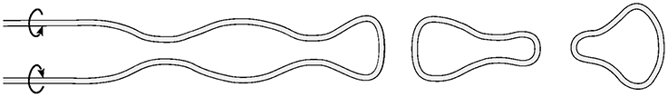
Figure 1. Sketch of the Crow instability in which anti-parallel vortex filaments develop into vortex rings through the reconnection process.

Here we discuss physical processes of vortex reconnection in superfluidity in the spirit of extracting the essence of reconnection and applying the knowledge to magnetic reconnection in space plasmas. It is worth emphasizing that both media are collisionless. A Bose-Einstein condensate is collisionless because of the large-scale coherence and the repulsive interaction potential between the constituting particles [12]. The space plasma is collisionless because of extremely low density. The frozen-in magnetic field condition may be compared to the circulation theorem in fluid dynamics (e.g., [13]). The conservation of the flow circulation is equivalent to the vortex equation,

$\begin{array}{cc}\frac{\partial \omega }{\partial t}=\nabla \times \left(u\times \omega \right),& (2)\end{array}$

where ω = ∇ × u denotes the vorticity. Equation (2) holds in an inviscid ordinary flow (cf. Euler equation). We seek the vortex equation for superfluidity, and compare with the induction equation under the generalized Ohm's law (Equation 1). The motivation for this comparison lies in the fact that the superfluid system has a smaller degree of freedom than plasmas, and thus, the vortex dynamics can be formulated in a simpler form. Such a form might inform us of some universal properties in collisionless reconnection. We review the fundamental equations describing the superfluid motion and discuss the vortex dynamics. We also review wave dynamics in the superfluid in association with with the vortex reconnection.

Before moving onto the comparison, it is worth mentioning that there may be several difficulties in the analogy between the vortex and magnetic reconnections. Among others, as the vorticity is the curl of the velocity, ω = ∇ × u, it is constrained to the velocity while the magnetic field not. In this sense, magnetic induction equation is more general than the vorticity counterpart. The analogy between the vorticity and magnetic inductions can be a sort of “one-way” character in that the general result obtained from the magnetic induction equation have a counterpart in the more particular context of the vorticity equation; In contrast, the result obtained from the vorticity induction equation may not have a counterpart in the more general context [14]. This point should be kept in mind when comparing the physics of reconnection between the superfluids and the collisionless plasmas. Also, the physical entities are different in that the vortex filaments are discrete while the magnetic fields are continuous.

2. Theoretical Treatment

In a superfluid, the rotational motion of the flow is associated with the vortex filament with a fixed circulation due to the quantization. The flow circulation is determined by the Planck constant (divided by 2π) ℏ and the mass of the constituting particle m as

$\begin{array}{cc}\kappa =\frac{2\pi \hslash }{m},& (3)\end{array}$

In addition, the quantum mechanical effect makes the vortex core size much smaller in the superfluid than in the ordinary fluid. The fixed circulation and the very thin filaments are unique to quantum vortex dynamics, first predicted by Feynman in 1955 [15] and later confirmed in the experiment by Vinen in 1961 [16]. The picture of vortex stretching breaks down in the superfluid, and vortex filament reconnection plays an essential role for the superfluid to evolve into turbulence. Recently, quantum vortex reconnection has been visualized in the superfluid helium experiments using tracing particles trapped by the vortex cores [17–19]. Figure 2 displays images of quantum vortex reconnection in the superfluid helium.

FIGURE 2

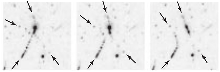
Figure 2. Images of vortex reconnection in superfluid helium as visualized by hydrogen particles suspended in liquid helium at 50-ms time intervals. Reproduced with permission from Bewley et al. [17]. Copyright (2008) National Academy of Sciences, U.S.A.

2.1. Kinetic Picture

2.1.1. Gross-Pitaevskii equation

Like in plasma physics or gas dynamics, both kinetic and fluid treatments are possible to describe the motion of a Bose-Einstein condensate. The kinetic picture is modeled by the non-linear Schrödinger equation or the Gross-Pitaevskii equation (hereafter GP) [20, 21]. The Schrödinger equation for N bosons with the mass m is written as

$\begin{array}{cc}\begin{array}{l}i\hslash \frac{\partial }{\partial t}\psi (x,t)+\frac{{\hslash }^2}{2m}{\nabla }^2\psi (x,t)-\psi (x,t){\displaystyle \int |}\psi (x^{\prime },t){|}^2\\ V(|x-x^{\prime }|)\text{d}{x}^{\prime }=0\end{array}& (4)\end{array}$

where V(|x − x′|) represents the interaction potential between two bosons. For weakly interacting bosons, one may approximate the repulsive potential to the delta function, and obtains the Gross-Pitaevskii equation in spatio-temporal coordinates as

$\begin{array}{cc}\text{i}\hslash \frac{\partial \psi }{\partial t}+\frac{{\hslash }^2}{2m}{\nabla }^2\psi -V_0|\psi {|}^2\psi +E_0\psi =0,& (5)\end{array}$

where V₀ denotes the coupling constant of the repulsive interaction. The chemical potential E₀ (the energy increment to the ground-state by adding one boson to the system) is included in the GP equation as the bosons are in a condensed state. The wavefunction ψ is normalized to the total number of particles N when integrated over the entire volume,

$\begin{array}{cc}{\displaystyle \int |\psi {|}^2{\text{d}}^{3}x}=N.& (6)\end{array}$

Note that the non-linearity in the GP equation originates in the repulsive interaction potential. The chemical potential E₀ is intrinsic to the Bose-Einstein condensate. Of course, the construction of the GP equation is different from that of the kinetic equations in plasma physics (e.g., Fokker-Planck, Boltzmann, or Vlasov equations) in that the GP equation does not represent the Liouville theorem on phase-space density conservation. The technical differences from the plasma kinetic equations can be summarized as follows: The velocity-space gradient is absent in the GP equation as the internal degree of freedom (in spins and energy levels) degenerates; The wavefunction ψ is complex due to the quantum mechanical phase; The equation is based on the Schrödinger equation, that is, the derivatives are asymmetric between the temporal and the spatial ones and the wavefunction ψ is intrinsically dispersive and not dissipative. The second-order spatial derivative causes dispersion of wave packets, while the non-linear self-interacting term causes localization of wave packets. Such a situation may be compared with a wave packet in the plasma under the ponderomotive force. The GP equation describes the superfluid dynamics on microscopic scales of the order of the vortex core radius. Vortex motion described by the non-linear Schrödinger-type equation is not unique to the superfluids but it appears in plasmas as well, e.g., in electron-positron plasmas [22].

2.1.2. Steady-state analysis

The steady-state solution for the GP equation is obtained by dropping the time-derivative term,

$\begin{array}{cc}\left(-\frac{{\hslash }^2}{2m}{\nabla }^2-E_0\right)\psi +V_0|\psi {|}^2\psi =0.& (7)\end{array}$

If the superfluid is homogeneous, one may even drop the spatial derivative to obtain the constant-value solution as ψ = f₀ = $\sqrt{\frac{E_0}{V_0}}$. What happens if the density distribution is inhomogeneous? The vortex core, naively speaking, represents a singularity at which the superfluid density is zero. We express the wavefunction using the radial part (or the amplitude) f and the phase θ as

$\begin{array}{cc}\psi =f(r){\text{e}}^{\text{i}\theta },& (8)\end{array}$

and obtain the steady-state equation for the amplitude f(r) by substituting into Equation (7),

$\begin{array}{cc}\frac{{\partial }^{2}f}{\partial r^2}+\frac{1}{r}\frac{\partial f}{\partial r}-\frac{f}{f^2}+\frac{2m}{{\hslash }^2}\left(E_{0}f-V_0{f}^3\right)=0.& (9)\end{array}$

The boundary condition is chosen as

$\begin{array}{cc}f=\{\begin{array}{ll}0\hfill & \text{for}r=0\hfill \\ \sqrt{\frac{E_0}{V_0}}\hfill & \text{as}r\to \infty .\hfill \end{array}& (10)\end{array}$

The steady-state radial equation (Equation 9) can be written in the dimensionless form as

$\begin{array}{cc}\frac{{\partial }^{2}g}{\partial s^2}+\frac{1}{s}\frac{\partial g}{\partial s}-\frac{g}{s^2}+g-g^3=0.& (11)\end{array}$

where the radial function f is normalized to the homogeneous steady-state solution as g = $\frac{f}{f_0}$, and the radial distance from the singularity r is normalized to the coherence length a₀ = $\frac{\hslash }{\sqrt{2m{E}_0}}$ as s = $\frac{r}{a_0}$. The existence of an analytic solution of Equation (11) for the entire spatial domain is not known, but the asymptotic behavior can be analyzed in the following way. First, in the vicinity of the singularity (s → 0), the non-linear term (with g³) is negligible, as g « 1 holds. The solution is given by the Bessel function of the first order, g = J₁(s). Second, at a large distance s → ∞, the radial function g is close to unity, and is obtained as g ≃ 1 − $\frac{1}{2s^2}$. The asymptotic behavior of the radial function f is therefore,

$\begin{array}{cc}f(r)=\{\begin{array}{ll}{f}_0{J}_1(\frac{r}{a_0})\simeq \frac{f_0}{2}\frac{r}{a_0}\hfill & \text{for}r\ll a_0\hfill \\ f_0\left(1-\frac{1}{2}{\left(\frac{a_0}{r^2}\right)}^2\right)\hfill & \text{as}r\to \infty .\hfill \end{array}& (12)\end{array}$

On the microscopic scale, the vortex core has a finite size of the order of the coherence length a₀. This fact comes directly from the uncertainty principle for considering condensate's momentum $p=\sqrt{2m{E}_0}$. Moreover, the fluid picture (explained below) indicates the existence of a void region (referred to as the topological defect) at the center of the core where the superfluidity state is broken in order to sustain the quantized circulation and the finite flow speed.

2.2. Fluid Picture

2.2.1. Madelung transformation

The fluid picture is obtained by applying the Madelung transformation [23] to the GP equation,

$\begin{array}{cc}\psi =f{\text{e}}^{\text{i}\theta }=f{\text{e}}^{\text{i}\frac{\hslash \varphi }{m}},& (13)\end{array}$

where the wavefunction phase ϕ is explicitely written using the coefficient ℏ/m. This transformation is useful in understanding superfluid dynamics, since the GP equation is converted into the form of compressible Euler equation [12, 24]. Two equations arise from the Madelung transformation. One is the continuity equation for the Bose-Einstein condensate density n (number density),

$\begin{array}{cc}\frac{\partial n}{\partial t}+\nabla ·\left(nu\right)=0,& (14)\end{array}$

and the other is the momentum equation,

$\begin{array}{cc}mn\left(\frac{\partial u}{\partial t}+u·\nabla u\right)=-\nabla p+\nabla ·\underset{\_}{\underset{\_}{\tau }}.& (15)\end{array}$

The number density n and the flow velocity u are given by the wavefunction ψ as

$\begin{array}{cc}n=\text{|}\psi {|}^2& (16)\end{array}$

$\begin{array}{cc}u=\frac{\hslash }{m}\nabla \varphi .& (17)\end{array}$

The absolute value of the wavefunction represents the square-root of density. The gradient of the wavefunction phase determines the flow velocity. The superfluid motion is a potential flow, and therefore, irrotational. The vorticity is zero everywhere as far as the superfluid exists:

$\begin{array}{cc}\omega =\nabla \times u=0.& (18)\end{array}$

This problem is discussed in more detail in the following section.

2.2.2. Quantum pressure

The pressure p is directly related to the density n (or mass density ρ) by

$\begin{array}{cc}p=\frac{V_0}{2m}{\rho }^2.& (19)\end{array}$

Equation (19) may be regarded as the equation of state for the Bose-Einstein condensate, and is intrinsic to the GP equation. It is worth noting that the concept of temperature does not appear in Equation (19). This fact is reminiscent of the adiabatic law p ∝ ρ^γ (using the polytropic index γ) or the equation of state for the degenerate matter, e.g., p ∝ n^5/3_e for the non-relativistic electron degeneracy pressure [25]. In plasmas, in contrast to the superfluid, the equation of state is not intrinsic to the fundamental equations, but is introduced to solve the closure problem when deriving the set of the fluid equations from the Vlasov equation by means of velocity moments. The pressure force (per unit mass) is arranged using the definition (Equation 19) as

$\begin{array}{cc}-\frac{1}{\rho }\frac{\partial p}{\partial x_i}=-\frac{V_0}{m^2}\frac{\partial \rho }{\partial x_i}.& (20)\end{array}$

With the help of the steady-state form (Equation 12), the asymptotic behavior of the density gradient is evaluated as follows:

$\begin{array}{cc}\frac{\partial \rho }{\partial x_i}=\{\begin{array}{ll}m{f}_0\frac{x_i}{2a_0^2}\hfill & \text{for}r\ll a_0\hfill \\ 2m{f}_0^2\left(1-\frac{a_0^2}{2r^2}\right)a_0^2\frac{x_i}{r^4}\hfill & \text{as}r\to \infty \hfill \end{array}& (21)\end{array}$

One can see that the density gradient becomes zero at a large distance due to the power-law dependence (r⁻⁴). At a small distance r « a₀, the pressure-gradient force is evaluated as

$\begin{array}{cc}-\frac{\partial \rho }{\partial x_i}=-\frac{V_0}{m}\frac{m{f}_0^2{x}_i}{2a_0^2}=-\frac{E_0^2}{{\hslash }^2}{x}_i.& (22)\end{array}$

2.2.3. Quantum stress

The quantum stress $\underset{\_}{\underset{\_}{\tau }}$ is unique to the Bose-Einstein condensates, and is given using the index notation as

$\begin{array}{cc}{\tau }_{ij}={\left(\frac{\hslash }{2m}\right)}^2\rho \frac{{\partial }^2}{\partial x_i\partial x_j}\ln \rho .& (23)\end{array}$

Both the quantum pressure-gradient force (−∇p) and the quantum stress-divergence force (∇ · $\underset{\_}{\underset{\_}{\tau }}$) in Equation (15) are acting in the attractive sense, that is, the force is in the inward direction to pinch the superfluid element onto the vortex core center. The stress force (per unit mass) is estimated in the same way as that for the pressure term. We first arrange the stress term:

$\begin{array}{cc}\begin{array}{l}\frac{1}{\rho }\frac{\partial {\tau }_{ij}}{\partial x_j}={\left(\frac{\hslash }{2m}\right)}^2[\frac{1}{{\rho }^3}\frac{\partial }{\partial x_i}\rho {\left(\frac{\partial \rho }{\partial x_j}\right)}^2-\frac{1}{{\rho }^2}\frac{\partial }{\partial x_i}\frac{\partial }{\partial x_j}\rho \left(\frac{\partial \rho }{\partial x_j}\right)-\\ \frac{1}{{\rho }^2}\frac{\partial }{\partial x_j}\frac{\partial }{\partial x_j}\rho \left(\frac{\partial \rho }{\partial x_i}\right)+\frac{1}{\rho }\frac{\partial }{\partial x_i}\frac{{\partial }^2\rho }{\partial x_j^2}],\end{array}& (24)\end{array}$

and then apply the asymptotic form of the density gradient (Equation 21) to obtain

$\begin{array}{cc}\frac{1}{\rho }\frac{\partial {\tau }_{ij}}{\partial x_j}=-4{\left(\frac{\hslash }{2m}\right)}^2\frac{x_i}{r^4}.& (25)\end{array}$

Both the pressure term (Equation 22) and the stress term (Equation 25) have the negative sign, implying that these forces are acting inward. The ratio of these terms is

$\begin{array}{cc}\frac{\left|-\nabla p\right|}{\left|\nabla ·\underset{\_}{\underset{\_}{\tau }}\right|}=\frac{1}{4}{\left(\frac{r}{a_0}\right)}^4& (26)\end{array}$

Thus, the fluid treatment is valid even within the vortex core (on the scale r < a₀), and furthermore, the quantum stress term plays by far a dominant role there. Moreover, the zero-vorticity (due to the potential flow) imposes that the divergence of the quantum stress must vanish. This makes a marked difference from the pressure tensor in plasma physics, in which the divergence of the pressure tensor can be non-zero, e.g., anisotropic pressure.

3. Vortex Dynamics

3.1. Small-Scale Picture

The circulation around the vortex line is quantized in the superfluid. The circulation is defined as line integration of the flow velocity along a closed trajectory C:

$\begin{array}{cc}\Gamma ={\displaystyle {\oint }_{\text{C}}u}·\text{d}r& (27)\end{array}$

If the contour is taken in a simply connected region (Figure 3 left), the line integration is replaced by the surface integration over the area S bounded by the contour C using the Stokes theorem. The circulation Γ^(s) vanishes due to the zero-vorticity,

$\begin{array}{cc}{\Gamma }^{(\text{s})}={\displaystyle {\int }_{\text{S}}\omega }·\text{d}S,& (28)\end{array}$

where the superscript (s) denotes the simply connected region. If the contour is taken in a multiply connected region (Figure 3 middle and right), the Stokes theorem cannot be applied. The circulation in the multiply connected region Γ^(m) is evaluated as

$\begin{array}{cc}{\Gamma }^{(\text{m})}=\frac{\hslash }{m}{\displaystyle {\oint }_{\text{C}}\nabla }\varphi ·\text{d}r=\frac{\hslash }{m}\Delta \varphi .& (29)\end{array}$

FIGURE 3

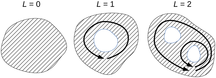
Figure 3. Simply connected region (left, genus L = 0) and multiply connected regions with the genus L = 1 (middle) and L = 2 (right).

The phase difference depends on the choice of contours. The wavefunction must remain a single-valued function $(\psi (x)=\psi (x){\text{e}}^{\text{i}\frac{\hslash \Delta \varphi }{m}})$, which yields the quantization of the circulation Γ,

$\begin{array}{cc}\begin{array}{l}\Gamma =\frac{2\pi \hslash }{m}L=\kappa L\\ (L=1,2,\cdots )\end{array}& (30)\end{array}$

The flow velocity in the azimuthal direction around the vortex line (assuming the axi-symmetric two-dimensional flow) is

$\begin{array}{cc}{u}_{\varphi }=\frac{\kappa }{2\pi r}L.& (31)\end{array}$

The divergence of the flow velocity in the small-distance limit (r → 0) is avoided by setting a cutoff in the distance. The cutoff represents topological defects (or holes) in the multiply connected region. In other words, the superfluid cannot exist inside the topological defect. The defect forms a continuous, smooth line connected to the system boundary (or the wall) or a closed curved line (vortex ring).

The kinetic energy stored in a unit-length vortex filament from the radius a₀ to R is estimated as

$\begin{array}{cc}E=\frac{1}{2}m{n}_0{\displaystyle {\int }_{a_0}^R{u}_{\varphi }^2}2\pi r\text{d}r& (32)\end{array}$

$\begin{array}{cc}=\frac{m{n}_0}{4\pi }{\left(L\kappa \right)}^2\ln \frac{R}{a_0}& (33)\end{array}$

where the number density n₀ is approximated to be constant. Equation (33) means that the flow energy becomes increasingly larger at a higher quantum number (L ≥ 2) as E ∝ L². The high-energy state of the superfluid vortices is relaxed by splitting into vortices at the lowest degree (L = 1). The flow energy is then proportional to the degree, E ∝ L, and is more stable. In fact, the vortex splitting has been confirmed in the numerical studies solving the GP equation [26–28]. Thus, the circulation in the superfluid plays as important role as the vorticity because the finite circulation originates from the topological defects. Ogawa et al. [29] argue that the circulation theorem breaks down in reconnection in that the effective pressure becomes indefinite at the reconnection point.

How can we compare the topological defects in the superfluid with the magnetic reconnection? Recently, Treumann et al. [30] revivied the idea of Aharonov-Bohm quantization [31]. The fundamental magnetic flux is evaluated for the electron motion around a flux tube (either using the cross section S or the orbit C) as

$\begin{array}{cc}\Phi ={\displaystyle {\int }_{\text{S}}B}·\text{d}S={\displaystyle {\oint }_{\text{C}}A}·\text{d}r& (34)\end{array}$

The magnetic field B is associated with the vector potential A by the relation B = ∇ × A, and the vector potential is further associated with the wavefunction phase by A = ∇ϕ. Again, the wavefunction must be single-valued, which results in the magnetic flux quantization to

$\begin{array}{cc}{\Phi }_0=\frac{2\pi \hslash }{e}& (35)\end{array}$

The smallest possible radius of the flux tube (or the radius of the magnetic field line) is then

$\begin{array}{cc}{\lambda }_{\text{m}}=\sqrt{\frac{{\Phi }_0}{\pi B}},& (36)\end{array}$

which gives the estimate of the topological defects in magnetic reconnection [30].

3.2. Large-Scale Picture

The problem of the zero-vorticity can be overcome with the coarse-graining method by grouping many vortex lines on the larger scale than the core size. The average separation distance between vortex lines ℓ is of the order of 1 μm in the ⁴He superfluid, and the system size (represented by the size of the largest eddies) is of the order of 10 mm [32]. On such a large scale, one may approximate the vorticity distribution using the three-dimensional delta function δ(x) as

$\begin{array}{cc}\omega (x)=\Gamma {\displaystyle \int \delta }\left(x-s(\xi )\right)\frac{ds}{d\xi }\text{d}\xi ,& (37)\end{array}$

where s denotes the curve of the filament parameterized by the one-dimensional coordinate ξ (the arc length) [33]. The flow velocity is then obtained by the Biot-Savart law for an irrotational motion [34–39],

$\begin{array}{cc}u=\frac{\Gamma }{4\pi }{\displaystyle \int \frac{(x^{\prime }-s)\times \text{d}{x}^{\prime }}{|x^{\prime }-s{|}^3}}.& (38)\end{array}$

By coarse-graining (bundling many vortex lines on a larger scale), one can treat the vorticity as an average, smoothed, and differentiable quantity. In such a treatment, the presence of turbulence plays a more essential role in violating the circulation theorem [40]. The coarse-grained vorticity is constructed in the same fashion as the method used in smoothed particle hydrodynamics [37–39, 41, 42] using the kernel or the smoothing function W:

$\begin{array}{cc}\overline{\omega }(x)={\displaystyle \int \omega }(x^{\prime })W(x-x^{\prime },\sigma )\text{d}{x}^{\prime }& (39)\end{array}$

$\begin{array}{cc}\simeq \kappa {\displaystyle \sum _{j=1}^N{\left(\frac{\text{d}s}{\text{d}\xi }\right)}_j}W(x-s_j,\sigma )\Delta {\xi }_j& (40)\end{array}$

where the smoothing W is a function of the distance between the two spatial positions and the smoothing length σ. One may choose the Gaussian shape or the polynomial form for the smoothing function.

The smoothed vorticity is meaningful if the vortex lines are locally polarized with non-zero alignment in some direction such that one can properly bundle many vortex lines. If the vortex lines are randomly and isotropically oriented in all the directions, the smoothed vorticity in a small fluid parcel will be zero (despite the fact that the vortex length inside that small parcel is not zero). But if the vortex lines are not random then a non-zero average vorticity exists. Figure 4 is an example of vortex bundles (in a numerical study using the GP equation) before and after reconnection. The wavy structure after reconnection represents the Kelvin waves associated with the vortex reconnection.

FIGURE 4

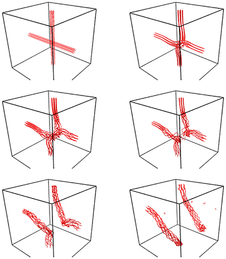
Figure 4. Numerical simulations of reconnecting vortex filament bundles in superfluid obtained by solving the Gross-Pitaevskii equation. Reprinted figure with permission from Alamri et al. [71]. Copyright (2008) by the American Physical Society.

One may incorporate the concept of turbulent viscosity into the smoothed vorticity dynamics. For the large-scale vorticity field, we apply the mean field decomposition as f = f + δf for the field f (e.g., flow velocity, density). The bar operator means averaging or smoothing. Taking the average of the fluid equation, and operating the curl, we obtain the equation for the mean vorticity field as

$\begin{array}{cc}\frac{\partial \overline{\omega }}{\partial t}=\nabla \times \left(\overline{u}\times \overline{\omega }\right)-\nabla \times \nabla \underset{\_}{\underset{\_}{R}},& (41)\end{array}$

where the matrix $\underset{\_}{\underset{\_}{R}}$ denotes the Reynolds stress defined as

$\begin{array}{cc}{R}_{ij}=\overline{\delta u_i\delta u_j}.& (42)\end{array}$

If the quantum fluid is set to fully-developed turbulence, one may further incorporate the one-point closure model or the Reynolds stress model as formulated by Boussinesq [43, 44],

$\begin{array}{cc}{R}_{ij}=-{\nu }_{\text{T}}\left(\frac{\partial {\overline{u}}_i}{\partial x_j}+\frac{\partial {\overline{u}}_j}{\partial x_i}\right)+\frac{2}{3}K{\delta }_{ij}& (43)\end{array}$

with the turbulent or eddy viscosity ν_T and the total kinetic energy K. The second-order derivative of the Reynolds stress term in the vortex equation then reduces to the turbulent dissipation (using the vector calculus identity that the divergence of the curl operator vanishes),

$\begin{array}{cc}\nabla \times \nabla \underset{\_}{\underset{\_}{R}}=-{\nu }_{\text{T}}{\nabla }^2\overline{\omega }.& (44)\end{array}$

To summarize, although the vorticity is zero on a microscopic scale, a bundle of non-zero circulations (that arises from the topological defects) gives a finite value of the smoothed vorticity on a macroscopic scale. The dynamics of the smoothed vorticity can be formulated using the turbulent viscosity, and as in the ordinary fluid dynamics, modeling of the Reynolds stress tensor is important here. Thus, comparison with the induction equation in plasmas (Equation 1) indicates that the anomalous resistivity η is most relevant to large-scale quantum vortex reconnection. It is worth while to note that the divergence of the pressure tensor must vanish in the superfluid, which is different from the plasma with the anisotropic pressure and non-zero stress tensor. The diffusivity coefficients need to be assessed by other means. One possibility is to derive the transport coefficients from the fundamental fluid equations (hydrodynamics, magnetohydrodynamics) on the basis of elaborated closure theory such as Direct Interaction Approximation (DIA) and Two-Scale Direct Interaction Approximation (TSDIA) [45–47]. Another possibility is to estimate the transport coefficients by incorporating wave-particle interactions for various resonance types and collision frequencies into the anomalous resistivity (e.g., [48]).

4. Wave Dynamics

Because of degeneracy in the spin state and the energy level, the superfluid has only two wave modes: Kelvin waves and sound waves. The former exhibits incompressible fluctuations acting on the tension of the vortex filaments, and the latter is compressible. There is no thermal or supra-thermal spread in the superfluid wavefunction, and thus, the wave-particle resonances or wave harmonics are absent. The lack of wave-particle resonances (more strictly, the lack of velocity-space gradient in the GP equation) is one of the differences from plasmas. This fact limits the possible wave modes in the superfluid only to Kelvin and sound waves.

4.1. Kelvin Wave

Kelvin waves [49] represent oscillations of the vortex filament with circular motions around the filament, and may be compared to Alfvén waves in plasmas. Dispersion relation of the Kelvin waves is expressed as

$\begin{array}{cc}{\omega }_{\text{K}}=\frac{\Gamma k_{\Vert }^2}{4\pi }\left[\ln \left(\frac{1}{k_{\Vert }{a}_0}\right)+c\right],& (45)\end{array}$

where ω_K denotes the Kelvin wave frequency. The symbol k‖ denotes the wavenumber in the direction to the vortex filament and c ≃ 1 [50–52]¹. Recently, the superfluid Kelvin waves have been revisited from the viewpoint of symmetry breakdown and restoration, and these waves can be formulated as realization of axi-symmetry restoration, known as the Nambu-Goldstone mode, [53].

The Kelvin waves evolve into turbulence by producing a series of daughter Kelvin waves as cascade. In addition to the vortex reconnection, Kelvin wave cascade serves as a channel or transport mechanism of fluctuation energy in the spectral domain. Superfluid turbulence is considered to show the formation of an inertial range or power-law regime in the energy spectrum [50, 54–57]. It is currently being discussed if the spectral slope exhibits that of Kolmogorov spectrum, −5/3, for reconnection-dominant superfluid turbulence [58] or if there are multiple inertial ranges from larger scales to smaller one [59].

The possibility of inverse energy cascade has also been predicted [60].

4.2. Sound Wave

Sound waves represent a compressible mode in the superfluid. This mode is dispersive in contrast to that in the ordinary fluid [24]. The dispersion relation is expressed as

$\begin{array}{cc}{\omega }_{\text{s}}^2=\frac{{\hslash }^2}{4m^2}{k}^4+\frac{E_0}{m}{k}^2,& (46)\end{array}$

where ω_s denotes the sound wave frequency, k the wavenumber. The first term represents the free-particle motion as is seen by reading the wavenumber as quasi-particle momentum, ℏk, and this term makes the sound wave dispersive. The second term represents the dispersionless phonons, ω ∝ c_sk, with the propagation speed $c_{\text{s}}=\sqrt{E_0/m}$. Depending on the spatial scale, the sound wave behaves like free particles or phonons. As is the case for the ordinary fluid, the superfluid sound mode does not have any preferred propagation direction, and in fact, and the waves propagate radially away from the reconnection site [24].

An important function of the sound waves is its involvement in the energy transfer mechanism. This mode exists even at the vanishing viscosity, and by exciting the sound waves, the kinetic energy in the turbulent superfluid flow can be converted into the sound energy. Numerical simulations of vortex tangles performed using the GP equation have shown that the fluctuation energy (or kinetic energy) decreases with time and the sound energy increases [61]. This is qualitatively in agreement with the equation of state (Equation 19) in that the density essentially replaces the role of temperature in superfluidity. Although viscosity is absent, the sound wave excitation serves as an effective energy dissipation mechanism [51].

5. Reconnection Processes

5.1. Before Reconnection

Two competing ideas exist to explain how reconnection sets on: the threshold model and the bifurcation model. The first approach is widely used in numerical studies of quantum vortex reconnection, e.g., [42, 62]. In this model, a critical distance is set as a parameter between two vortex filaments. The algorithm is implemented in such a way that two filaments merge and reconnect automatically whenever they meet at the critical distance. This distance is chosen typically of the order of the core size of filaments [63]. The second approach is based on the analytic solution obtained by linearizing the GP equation around the reconnecting point [64, 65],

$\begin{array}{cc}\psi (r,t)=a_{\text{x}}{x}^2-a_{\text{y}}{y}^2+\left(a_{\text{z}}+\text{i}\right)z-2\text{i}(a_{\text{x}}-a_{\text{y}})(t-t_0)& (47)\end{array}$

where the spatial coordinate r = (x, y, z) is centered at the reconnection point at (0, 0, 0) and spanned by the two reconnecting vortex filaments (assumed to be co-planar, x-y plane). t₀ denotes the bifurcation or reconnection time. The coefficients a_x, a_y, and a_z are positive constants, and satisfy the condition a_x > a_y. The wavefunction represents a set of hyperbolae parameterized by the coefficients, and is a smooth function in space and time even at the reconnection point. Before bifurcation (t < t₀) and after that (t > t₀) the vortex filaments are given by two hyperbolae (obtained by the condition ψ = 0) in the x-y plane. At the reconnection time, the hyperbolae degenerate to two intersecting straight lines. No wave activity is needed to mediate the reconnection onset, but the reconnection is induced by the dispersion effect (the second-order spatial derivative) in the GP equation.

Reconnecting filaments exhibit a scaling law in their minimum distance. The scaling law is obtained on the assumption that the circulation Γ is the only relevant parameter [66, 67] as

$\begin{array}{cc}d=D{\left[\Gamma \left|t_0-t\right|\right]}^{\alpha },& (48)\end{array}$

where the coefficient D is a dimensionless parameter. Numerical simulation and analytic model predict the value of D around 0.4 [68, 69] and the power-law index α = 1/2 [66, 67]. This index value can also be derived from the bifurcation model [64].

In the numerical simulations solving the GP equation, the index α is yet different across the reconnection event: α ≃ 0.4 and α ≃ 0.7 before and after the reconnection, respectively [24]. Just before reconnection occurs, the two vortex filaments form a co-planar configuration with the opposite sense of vortex (in other words, anti-parallel filaments) by tilting the axes of filaments locally [65]. When many vortex filaments exists, reconnection occurs in a successive fashion. Reconnection rate ν can then be scaled to the vortex line density Φ by the relation ν ∝ Φ^5/2 [70]. No wave activity is observed before the reconnection event, and waves are observed together with the reconnection event. This result indicates that the waves are the product of reconnection.

5.2. After Reconnection

Figure 4 displays the evolution of vortex filaments (or bundles) before and after reconnection [71]. The Kelvin waves are excited when the bundles reconnect, as visualized by oscillation or entanglement of the vortex filaments. The generated Kelvin waves develop into turbulence [72]. Moreover, recent experiment by Fonda et al. [73] provides for the first time the evidence that the Kelvin waves are excited by quantum vortex reconnection. Not only the Kelvin waves but also the sound waves are excited after reconnection as a pulse, propagating in the radial direction away from the reconnection point [24, 29, 74]. Wave emission means the energy loss. Quantum vortex reconnection is an asymmetric process with respect to the time reversal, i.e., the reconnected vortex filaments cannot simply be put back to the initial un-reconnected state because the filament distortion (by the Kelvin waves) and the pulse emission (by the sound waves) carry the energy away from the reconnection point. In addition, the distance scaling index α is different across the reconnection time (α ≃ 0.4 and α ≃ 0.7 before and after reconnection, respectively) [24] such that the reconnected filaments deviate from each other more rapidly than they approach to reconnection.

6. Lessons

On one hand, one may critically view that the comparison between vortex reconnection in the superfluid and magnetic reconnection in the plasma might not be useful in the first place because of the lack of internal degree of freedom in the superfluid. In fact, on the microscopic scale, the vorticity is strictly zero due to the nature of the potential flow. On the other hand, one can find similarities in the reconnection process between the two media both on the microscopic and the macroscopic levels. To summarize, the lessons from quantum vortex reconnection are as follows.

1. Quantum vortex reconnection is controlled by the physics of topological defects on the microscopic scale, and by the physics of turbulence on the macroscopic scale.

2. Due to the irrotational property of the superfluid motion, the quantum pressure or stress forces cannot trigger reconnection by themselves. Non-zero flow circulation in the superfluid comes from the topological defects (such as impurity or breakdown of the superfluidity). The quantized magnetic flux may be compared with the topological defects in the superfluid. Physics of reconnection trigger reduces to physics of topological defects on a microscopic scale.

3. On the larger scales, the dynamics of smoothed vorticity can be compared with the generalized Ohm's law for the plasma. The existence of turbulence is important in that the turbulent fluctuation serves an effective dissipation mechanism.

4. Non-linearity is sufficiently small and the linearization of the fundamental equation is a valid approach. Quantum vortex reconnection can be obtained as an analytic solution of the linearized GP equation, and there, the dispersion effect (broadening of the wave packets or the density in the direction of propagation) is essential in the analytic solution of quantum vortex reconnection.

5. Waves themselves are not likely the primary mechanism causing reconnection. However, wave emission (Kelvin waves and sound waves) are observed together with the vortex reconnection. Furthermore, the excitation of sound waves serves as an effective dissipation mechanism. It is possible that waves excitation is involved on a fundamental level in magnetic reconnection.

6. Waves carry a portion of the energy away from the reconnection site and make reconnection asymmetric to time reversal. The question remains, however, as to the exact timing of wave emission. Waves may be excited at the same time as reconnection or may be after reconnection.

What is the implications of quantum vortex reconnection to magnetic reconnection in space plasmas? The generalized Ohm's law in plasmas shows different possible causes of the breakdown of the frozen-in magnetic field condition: Hall effect, anisotropic pressure and stress of the electron fluid, electron inertia, and anomalous resistivity. Even though the fluid equations for the superfluidity has the pressure-gradient term and the divergence of the stress tensor, they cannot induce the quantum vortex reconnection on the microscopic scale. Theoretical consideration of anomalous resistivity in plasmas leads to the conclusion that waves or turbulent fluctuations are one of the likely candidates to trigger magnetic reconnection. Various kinds of wave modes are proposed as the mechanism of the anomalous resistivity, e.g., Buneman wave, ion acoustic wave, Langmuir wave, lower-hybrid drift wave, and cyclotron wave as reviewed in Treumann [48]. For a proper evaluation of the generalized Ohm's law, it is necessary to identify wave modes and their interaction with particles, and to compare with these other contributions. In the spacecraft observations in situ in space, wave modes can unambiguously be determined by investigating the existence of dispersion relation, namely, the energy spectrum in the wavevector-frequency domain. Multi-spacecraft missions provide us with the very opportunity for such a task, and the combination between the wave analysis and the evaluation of the generalized Ohm's law will serve as a powerful tool to solve the reconnection onset problem in collisionless magnetic reconnection.

Turbulence has dual effects. That is, turbulence serves not only as an effective dissipation mechanism (through eddy viscosity) but also as a mechanism of transport suppression or even large-scale structure formation. A typical situation is the turbulent dynamo in which the helicity quantities (magnetic helicity, kinetic helicity, and cross helicity) play an essential role when symmetries in the system such as rotation or magnetic field topology (e.g., spatial inversion or non-mirror symmetry) break down. The structure formation (or the magnetic field generation) proceeds in a turbulent medium while the primary effect of turbulence still lies in enhancing the magnetic diffusion. Such dual effects of turbulence are indeed presented in recent studies of turbulent magnetic reconnection [47, 75] While we have compared the generalized Ohm's law in a plasma with the vortex equation in a superfluid, such a comparison work should be extended to the symmetry breakdown associated with the helicity quantities (kinetic helicity evolution across vortex filament reconnection, magnetic and cross helicities across magnetic reconnection).

Author Contributions

Yasuhito Narita drafting the work; Wolfgang Baumjohann substantial contributions to the design of the work. We acknowledge Prof. Tohru Nakano for sharing the lecture notes on quantum turbulence (2008) for the detailed calculations in the GP equation.

Conflict of Interest Statement

The authors declare that the research was conducted in the absence of any commercial or financial relationships that could be construed as a potential conflict of interest.

Footnotes

1. ^The symbol ω is commonly used both for the vorticity and for the angular frequency. We keep the notation style as these two quantities are not mixed in the manuscript.

References

1. Sweet PA. The neutral point theory of solar flare. In: Lehnert B, editor. IAU Symposium 6, Electromagnetic Phenomena in Cosmical Physics. Dordrecht: Kluwer (1958). p. 123–34.

2. Parker EN. Sweet's mechanism for merging magnetic fields in conducting fluids. J Geophys Res. (1957) 62:509–20. doi: 10.1029/JZ062i004p00509

CrossRef Full Text | Google Scholar

3. Petschek HE. Magnetic field annihilation. In: The Physics of Solar Flares, Proceedings of the AAS-NASA Symposium 2830 October 1963 at Goddard Space Flight Center Greenbelt. Greenbelt, MD: NASA (1964). p. 425–39.

4. Treumann R, Baumjohann W. Collisionless magnetic reconnection in space plasmas. Front Phys. (2013) 1:31. doi: 10.3389/fphy.2013.00031

CrossRef Full Text | Google Scholar

5. Zweibel EG, Yamada M. Magnetic reconnection in astrophysical and laboratory plasmas. Ann Rev Astron Astrophys. (2009) 47:291–332. doi: 10.1146/annurev-astro-082708-101726

CrossRef Full Text | Google Scholar

6. Yamada M, Kulsrud R, Ji H. Magnetic reconnection. Rev Mod Phys. (2010) 82:603–64. doi: 10.1103/RevModPhys.82.603

CrossRef Full Text | Google Scholar

7. Rossi B, Olbert S. Introduction to the Physics of Space. New York, NY: McGraw-Hill (1970).

Google Scholar

8. Baumjohann W, Treumann RA. Basis Space Plasma Physics, Revised. London: Imperial College Press (2012).

9. Crow SC. Stability theory for a pair of trailing vortices. Amer Inst Aeronautics Astronautics. (1970) 8:2172–9. doi: 10.2514/3.6083

CrossRef Full Text | Google Scholar

10. Van Dyke M. Album of Fluid Motion. Stanford, CA: Parabolic Press (1982).

Google Scholar

11. Takaki R. Reconnection of line singularities – Description and mechanism. Forma. (2002) 17:211–38.

Google Scholar

12. Roberts PH, Berloff NG. The nonlinear Schrödinger equation as a model of superfluidity. Quantized vortex dynamics and superfluid turbulence. Lect. Notes Phys. (2001) 571:235–57.

Google Scholar

13. Choudhuri AR. The Physics of Fluids and Plasmas, An Introduction for Astrophysicists. Cambridge: Cambridge University Press (1998).

Google Scholar

14. Moffatt HK. Magnetic Field Generation in Electrically Conducting Fluids. Cambridge: Cambridge University Press (1978).

15. Feynman RP. Application of quantum mechanics to liquid helium. In: Gorter CJ, editor. Progress in Low Temperature Physics. Vol. 1. Amsterdam: North Holland (1955). p. 17–53.

16. Vinen WF. The detection of single quanta of circulation in liquid helium II. Proc Roy Soc A. (1961) 260:218–36. doi: 10.1098/rspa.1961.0029

CrossRef Full Text | Google Scholar

17. Bewley GP, Paoletti MS, Sreenivasan KR, Lathrop DP. Characterization of reconnecting vortices in superfluid helium. Proc Natl Acad Sci USA. (2008) 105:13707–10. doi: 10.1073/pnas.0806002105

Pubmed Abstract | Pubmed Full Text | CrossRef Full Text | Google Scholar

18. Paoletti MS, Fisher ME, Sreenivasan KR, Lathrop DP. Velocity statistics distinguish quantum turbulence from classical turbulence. Phys Rev Lett. (2008) 101:154501. doi: 10.1103/PhysRevLett.101.154501

Pubmed Abstract | Pubmed Full Text | CrossRef Full Text | Google Scholar

19. Paoletti MS, Fisher ME, Lathrop DP. Reconnection dynamics for quantized vortices. Physica D. (2010) 239:1367–77. doi: 10.1016/j.physd.2009.03.006

CrossRef Full Text | Google Scholar

20. Ginzburg VL, Pitaevskii LP. On the theory of superfluidity. Zh Eksp Teor Fiz. (1958) 34:1240.

Google Scholar

21. Gross EP. Hydrodynamics of a superfluid condensate. J Math Phys. (1963) 4:195–207. doi: 10.1063/1.1703944

CrossRef Full Text | Google Scholar

22. Tatsuno T, Berezhiani VI, Mahajan SM. Vortex solitons: mass, energy, and angular momentum bunching in relativistic electron-positron plasmas. Phys Rev E. (2001) 63:046403. doi: 10.1103/PhysRevE.63.046403

Pubmed Abstract | Pubmed Full Text | CrossRef Full Text | Google Scholar

23. Madelung E. Quantentheorie in hydrodynamischer Form. Zeitschrift für Physik. (1927) 40:322–6. doi: 10.1007/BF01400372

CrossRef Full Text | Google Scholar

24. Zuccher S, Caliari M, Baggaley AW, Barenghi CF. Quantum vortex reconnections. Phys Fluids. (2012) 24:125108. doi: 10.1063/1.4772198

CrossRef Full Text | Google Scholar

25. Shapiro SL, Teukolsky SA. Black Holes, White Dwarfs, and Neutron Stars. The Physics of Compact Objects. New York, NY: Wiley (1983).

Google Scholar

26. Kawaguchi Y, Ohmi T. Splitting instability of a multiply charged vortex in a Bose-Einstein condensate. Phys Rev A. (2004) 70:043610. doi: 10.1103/PhysRevA.70.043610

CrossRef Full Text | Google Scholar

27. Saito H, Ueda M. Split-merge cycle, fragmented collapse, and vortex disintegration in rotating Bose-Einstein condensates with attractive interactions. Phys Rev A. (2004) 69:013604. doi: 10.1103/PhysRevA.69.013604

CrossRef Full Text | Google Scholar

28. Huhtamäki JAM, Möttönen M, Isoshima T, Pietilä V, Virtanen SMM. Splitting times of doubly quantized vortices in dilute Bose-Einstein condensates. Phys Rev Lett. (2006) 97:110406. doi: 10.1103/PhysRevLett.97.110406

Pubmed Abstract | Pubmed Full Text | CrossRef Full Text | Google Scholar

29. Ogawa S, Tsubota M, Hattori Y. Study of reconnection and acoustic emission of quantized vortices in superfluid by the numerical analysis of the GrossPitaevskii equation. J Phys Soc Jpn. (2002) 71:813–21. doi: 10.1143/JPSJ.71.813

CrossRef Full Text | Google Scholar

30. Treumann RA, Nakamura R, Baumjohann W. Flux quanta, magnetic field lines, merging - some sub-microscale relations of interest in space plasma physics. Ann Geophys. (2011) 29:1121–7. doi: 10.5194/angeo-29-1121-2011

CrossRef Full Text | Google Scholar

31. Aharonov Y, Bohm D. Significance of electromagnetic potentials in the quantum theory. Phys Rev. (1959) 115:485–91. doi: 10.1103/PhysRev.115.485

CrossRef Full Text | Google Scholar

32. Barenghi CF, L'vov VS, Roche PE. Experimental, numerical, and analytical velocity spectra in turbulent quantum fluid. Proc Natl Acad Sci USA. (2014) 111(Suppl. 1):4683–90. doi: 10.1073/pnas.1312548111

Pubmed Abstract | Pubmed Full Text | CrossRef Full Text | Google Scholar

33. Tsubota M. Quantum turbulence. J Phys Soc Jpn. (2008) 77:111006. doi: 10.1143/JPSJ.77.111006

CrossRef Full Text | Google Scholar

34. Ashurst WT, Meiron DI. Numerical study of vortex reconnection. Phys Rev Lett. (1987) 58:1632–5. doi: 10.1103/PhysRevLett.58.1632

Pubmed Abstract | Pubmed Full Text | CrossRef Full Text | Google Scholar

35. Saffman PG. Vortex Dynamics. Cambridge: Cambridge University Press (1992).

Google Scholar

36. Alamri SZ, Arenezi AA. Reconnection of vortex bundles lines with sinusoidally. Appl Math. (2013) 4:945–9. doi: 10.4236/am.2013.46130

CrossRef Full Text | Google Scholar

37. Baggaley AW, Laurie J, Barenghi CF. Vortex-density fluctuations, energy spectra, and vortical regions in superfluid turbulence. Phys Rev Lett. (2012) 109:205304. doi: 10.1103/PhysRevLett.109.205304

Pubmed Abstract | Pubmed Full Text | CrossRef Full Text | Google Scholar

38. Baggaley AW, Barenghi CF, Shukurov A, Sergeev YA. Coherent vortex structures in quantum turbulence. Europhys Lett. (2012) 98:26002. doi: 10.1209/0295-5075/98/26002

Pubmed Abstract | Pubmed Full Text | CrossRef Full Text | Google Scholar

39. Baggaley AW. The importance of vortex bundles in quantum turbulence at absolute zero. Phys Fluids. (2012) 24:055109. doi: 10.1063/1.4719158

CrossRef Full Text | Google Scholar

40. Chen S, Eyink GL, Wan M, Xiao Z. Is the Kelvin theorem valid for high Reynolds number turbulence? Phys Rev Lett. (2006) 97:144505. doi: 10.1103/PhysRevLett.97.144505

Pubmed Abstract | Pubmed Full Text | CrossRef Full Text | Google Scholar

41. Monaghan JJ. Smoothed particle hydrodynamics. Ann Rev Astron Astrophys. (1992) 30:543–74. doi: 10.1146/annurev.aa.30.090192.002551

CrossRef Full Text | Google Scholar

42. Barenghi CF, Samuels DC, Bauer GH, Donnelly RJ. Superfluid vortex lines in a model of turbulent flow. Phys Fluids. (1997) 9:2631–43. doi: 10.1063/1.869379

CrossRef Full Text | Google Scholar

43. Boussinesq J. Essai sur la théorie des eaux courantes. Mémoires présentés par divers savants à l'Académie des Sciences. (1877) 23:1–680.

44. Schmitt FG. About Boussinesq's turbulent viscosity hypothesis: historical remarks and a direct evaluation of its validity. Comptes Rendus Mécanique. (2007) 335:617–27. doi: 10.1016/j.crme.2007.08.004

CrossRef Full Text | Google Scholar

45. Kraichnan RH. Isotropic turbulence and inertial-range structure. Phys Fluids. (1966) 9:1728–52. doi: 10.1063/1.1761928

CrossRef Full Text | Google Scholar

46. Yoshizawa A. Statistical analysis of the deviation of the Reynolds stress from its eddy-viscosity representation. Phys Fluids. (1984) 27:1377–87. doi: 10.1063/1.864780

CrossRef Full Text | Google Scholar

47. Yokoi N. Cross helicity and related dynamo. Geophys Astrophys Fluid Mech. (2013) 107:114–84. doi: 10.1080/03091929.2012.754022

CrossRef Full Text | Google Scholar

48. Treumann RA. Origin of resistivity in reconnection. Earth Planets Space. (2001) 53:453–62. doi: 10.1186/BF03353256

Pubmed Abstract | Pubmed Full Text | CrossRef Full Text | Google Scholar

49. Thomson SW. Vibrations of a columnar vortex. Phil Mag Ser. (1880) 10:155–68. doi: 10.1080/14786448008626912

CrossRef Full Text | Google Scholar

50. Vinen WF, Tsubota M, Mitani A. Kelvin-wave cascade on a vortex in superfluid ⁴He at a very low temperature. Rev Rev Lett. (2003) 91:135301. doi: 10.1103/PhysRevLett.91.135301

Pubmed Abstract | Pubmed Full Text | CrossRef Full Text | Google Scholar

51. Barenghi CF. Turbulent dissipation near absolute zero. Eur J Mech B Fluids. (2004) 23:415–25. doi: 10.1016/j.euromechflu.2003.10.011

CrossRef Full Text | Google Scholar

52. Paoletti MS, Lathrop DP. Quantum turbulence. Ann Rev Condens Matter Phys. (2011) 2:213–34. doi: 10.1146/annurev-conmatphys-062910-140533

CrossRef Full Text | Google Scholar

53. Kobayashi M, Nitta M. Kelvin modes as Nambu-Goldstone modes along superfluid vortices and relativistic strings: finite volume size effects. Prog Theor Exp Phys. (2014) 2014:021B01. doi: 10.1093/ptep/ptu017

CrossRef Full Text | Google Scholar

54. Kivotides D, Vassilicos JC, Samuels DC, Barenghi CF. Kelvin waves cascade in superfluid turbulence. Phys Rev Lett. (2001) 86:3080–3. doi: 10.1103/PhysRevLett.86.3080

Pubmed Abstract | Pubmed Full Text | CrossRef Full Text | Google Scholar

55. L'vov VS, Nazarenko SV, Skrbek L. Energy spectra of developed turbulence in helium superfluids. J Low Temp Phys. (2006) 145:125–42. doi: 10.1007/s10909-006-9230-8

CrossRef Full Text | Google Scholar

56. Boffetta G, Celani A, Dezzani D, Lauire J, Nazarenko S. Modeling Kelvin wave cascades in superfluid helium. J Low Temp Phys. (2009) 156:193–214. doi: 10.1007/s10909-009-9895-x

CrossRef Full Text | Google Scholar

57. Baggaley AW, Barenghi CF. Spectrum of turbulent Kelvin-waves cascade in superfluid helium. Phys Rev B. (2011) 83:134509. doi: 10.1103/PhysRevB.83.134509

Pubmed Abstract | Pubmed Full Text | CrossRef Full Text | Google Scholar

58. Kivotides D, Leonard A. Quantized turbulence physics. Phys Rev Lett. (2003) 90:234503. doi: 10.1103/PhysRevLett.90.234503

Pubmed Abstract | Pubmed Full Text | CrossRef Full Text | Google Scholar

59. Kozik E, Svistunov B. Kolmogorov and Kelvin-wave cascades of superfluid turbulence at T = 0: what lies between. Phys Rev B. (2008) 77:060502. doi: 10.1103/PhysRevB.77.060502

Pubmed Abstract | Pubmed Full Text | CrossRef Full Text | Google Scholar

60. Baggaley AW, Barenghi CF, Sergeev YA. Three-dimensional inverse energy transfer induced by vortex reconnections. Phys Rev E. (2014) 89:013002. doi: 10.1103/PhysRevE.89.013002

Pubmed Abstract | Pubmed Full Text | CrossRef Full Text | Google Scholar

61. Nore C, Abid M, Brachet ME. Kolmogorov turbulence in low temperatures superflows. Phys Rev Lett. (1997) 78:3896–9. doi: 10.1103/PhysRevLett.78.3896

CrossRef Full Text | Google Scholar

62. Hänninen R. Dissipation enhancement from a single vortex reconnection in superfluid helium. Phys Rev B. (2013) 88:054511. doi: 10.1103/PhysRevB.88.054511

CrossRef Full Text | Google Scholar

63. Koplik J, Levine H. Vortex reconnection in superfluid helium. Phys Rev Lett. (1993) 71:1375–8.

Pubmed Abstract | Pubmed Full Text | Google Scholar

64. Nazarenko S, West R. Analytical solution for nonliner Schrödinger vortex reconnection. J Low Temp Phys. (2003) 132:1. doi: 10.1023/A:1023719007403

CrossRef Full Text | Google Scholar

65. Berry MV, Dennis MR. Reconnections of wave vortex lines. Eur J Phys. (2012) 33:723–31. doi: 10.1088/0143-0807/33/3/723

Pubmed Abstract | Pubmed Full Text | CrossRef Full Text | Google Scholar

66. Siggia ED. Collapse and amplification of a vortex filament. Phys Fluids. (1985) 28:794–805. doi: 10.1063/1.865047

CrossRef Full Text | Google Scholar

67. Schwartz KW. Three-dimensional vortex dynamics in superfluid ⁴He: line-line and line-boundary interactions. Phys Rev B. (1985) 31:5782–804. doi: 10.1103/PhysRevB.31.5782

Pubmed Abstract | Pubmed Full Text | CrossRef Full Text | Google Scholar

68. de Waele ATAM, Aarts RGKM. Route to vortex reconnection. Phys Rev Lett. (1994) 72:482–5. doi: 10.1103/PhysRevLett.72.482

Pubmed Abstract | Pubmed Full Text | CrossRef Full Text | Google Scholar

69. Boué L, Khomenko D, L'vov VS, Procaccia I. Analytic solution of the approach of quantum vortices towards reconnection. Phys Rev Lett. (2013) 111:145302. doi: 10.1103/PhysRevLett.111.145302

Pubmed Abstract | Pubmed Full Text | CrossRef Full Text | Google Scholar

70. Barenghi CF, Samuels DC. Scaling laws of vortex reconnections. J Low Temp Phys. (2004) 136:281–93. doi: 10.1023/B:JOLT.0000041267.08268.7a

CrossRef Full Text | Google Scholar

71. Alamri SZ, Youd AJ, Barenghi CF. Reconnection of superfluid vortex bundles. Phys Rev Lett. (2008) 101:215302. doi: 10.1103/PhysRevLett.101.215302

Pubmed Abstract | Pubmed Full Text | CrossRef Full Text | Google Scholar

72. Leadbeater M, Samuels DC, Barenghi CF, Adams CS. Decay of superfluid turbulence via Kelvin-wave radiation. Phys Rev A. (2003) 67:015601. doi: 10.1103/PhysRevA.67.015601

Pubmed Abstract | Pubmed Full Text | CrossRef Full Text | Google Scholar

73. Fonda E, Meichle DP, Ouellette NT, Hormoz S, Lathrop DP. Direct observation of Kelvin waves excited by quantized vortex reconnection. Proc Natl Acad Sci USA. (1998) 111(Suppl. 1):4707–10. doi: 10.1073/pnas.1312536110

Pubmed Abstract | Pubmed Full Text | CrossRef Full Text | Google Scholar

74. Leadbeater M, Winiecki T, Samuels DC, Barenghi CF, Adams CS. Sound emission due to superfluid vortex reconnections. Phys Rev Lett. (2001) 86:1410–3. doi: 10.1103/PhysRevLett.86.1410

Pubmed Abstract | Pubmed Full Text | CrossRef Full Text | Google Scholar

75. Yokoi N, Higashimori K, Hoshino M. Transport enhancement and suppression in turbulent magnetic reconnection: a self-consistent turbulence model. Phys Plasmas. (2013) 20:122310. doi: 10.1063/1.4851976

CrossRef Full Text | Google Scholar

76. Rogel-Salazar J. The Gross-Pitaevskii equation and Bose-Einstein condensates. Eur J Phys. (2013) 34:247–57. doi: 10.1088/0143-0807/34/2/247

CrossRef Full Text | Google Scholar

Appendix: Derivation of Fluid Equations

The set of the fluid equations is obtained from the GP equation as follows (see also [76]). We apply the Madelung transformation (Equation 13) to the GP equation (Equation 5):

$\begin{array}{cc}\begin{array}{l}\text{i}\hslash \left[\dot{f}+\frac{\text{i}m}{\hslash }f\dot{\varphi }\right]=-\frac{{\hslash }^2}{2m}[{\nabla }^{2}f+\frac{\text{i}m}{\hslash }f{\nabla }^2\varphi +2\frac{\text{i}m}{\hslash }\left(\nabla f\right)·\left(\nabla \varphi \right)\\ -{\left(\frac{m}{\hslash }\right)}^{2}f{\left(\nabla \varphi \right)}^2]\\ -E_{0}f+V_0{f}^3,\end{array}& (\text{A}1)\end{array}$

where the dot operation such as $\dot{f}$ or $\dot{\varphi }$ means the time derivative. The imaginary part of the above equation (Equation A1) reads

$\begin{array}{cc}\hslash \dot{f}=-\frac{\hslash }{2}f{\nabla }^2\varphi -\hslash \left(\nabla f\right)·\left(\nabla \varphi \right).& (\text{A}2)\end{array}$

The real part reads

$\begin{array}{cc}-mf\dot{\varphi }=-\frac{{\hslash }^2}{2m}\left[{\nabla }^{2}f-{\left(\frac{m}{\hslash }\right)}^{2}f{\left(\nabla \varphi \right)}^2\right]-E_{0}f+V_0{f}^3& (\text{A}3)\end{array}$

or, after arrangement,

$\begin{array}{cc}\dot{\varphi }+\frac{1}{2}{\left(\nabla \varphi \right)}^2-\frac{E_0}{m}+\frac{V_0}{m}{f}^2-\frac{{\hslash }^2}{2m}\frac{1}{f}\nabla f=0& (\text{A}4)\end{array}$

The continuity equation (Equation 14) is obtained by using the variables for the density n (Equation 16) and the flow velocity u (Equation 17). The momentum equation is obtained by taking the gradient of Equation (A4).