The Importance of Environmental Exposure History in Forecasting Dungeness Crab Megalopae Occurrence Using J-SCOPE, a High-Resolution Model for the US Pacific Northwest

Introduction

The Dungeness crab fishery is one of the most economically important fisheries on the US West Coast, totaling over $200M in 2017 (Pacific States Marine Fisheries Commission, 2019). However, this fishery experiences wide inter-annual fluctuations in catch size. For example, in Washington and Oregon, the lowest commercial crab catches were reported in the early 1980s (<1300 metric tons in Washington; <2300 metric tons in Oregon), and record high catches, nearly 10-fold higher, were reported in the 2004–2005 season (>11,300 metric tons in Washington; >15,000 metric tons in Oregon), with moderate variability observed even across consecutive years.¹, ² Variable catch rates have been accompanied by large swings in ex-vessel landing values, e.g. from $33.9M in the 2013–2014 season to $74.2M in the 2017–2018 season in Oregon. These large fluctuations have the potential to affect management strategies, fishermen’s livelihoods, and local economies (Botsford et al., 1983; Methot, 1986). Due to consistently high fishing effort, it is thought that variable annual catch rates reflect changes in adult Dungeness crab population sizes. The precise causes of this variability are not completely understood but have long been a subject of research (Methot and Botsford, 1982; Botsford and Hobbs, 1995; Higgins et al., 1997).

One factor that has been linked to variability in the Metacarcinus magister fishery is the abundance of the final pelagic larval stage, the megalopal stage, 4 years prior (Shanks and Roegner, 2007; Shanks et al., 2010; Shanks, 2013). Shanks (2013) reported a significant, parabolic relationship between megalopae abundance in coastal habitats and recruitment into the adult M. magister fishery four years later: recruitment into the fishery was maximized at intermediate megalopae abundances, and otherwise was limited either by population levels (low abundance) or density-dependent effects (high abundance).

Abundance of M. magister megalopae is influenced by ocean conditions on small and large scales. For example, survival and condition of M. magister larvae have been shown to be negatively impacted by exposure to low pH (Descoteaux, 2014; Miller et al., 2016); steep calcite saturation state gradients (Bednaršek et al., 2020); extreme temperatures (Wild, 1980; Pauley et al., 1989; Sulkin et al., 1996); low salinities (Reed, 1969; Brown and Terwilliger, 1999); low oxygen conditions (Bancroft, 2015; Gossner, 2018); and poor-quality or scarce food (Bigford, 1977; Harms and Seeger, 1989; Sulkin et al., 1998; Casper, 2013). Additionally, megalopae abundance has been significantly correlated with large-scale oceanographic features, such as the phase of the Pacific Decadal Oscillation (PDO; Shanks, 2013), wind-induced currents (Hobbs et al., 1992), and the timing of the spring transition of the California Current (Shanks and Roegner, 2007). The spring transition marks the onset of seasonal upwelling, which is a primary driver of ocean variability in this region.

Every summer the coastline of the Pacific Northwest experiences a shift in wind direction that promotes upwelling of “corrosive” deep water, which is low in oxygen, pH, and calcium carbonate saturation states, to habitat on the continental shelf (Huyer et al., 1979; Feely et al., 2008, 2016; Hickey and Banas, 2008). Though these winds vary in intensity and duration, hypoxia (O₂ < 1.4 ml l^–1; 61 μmol kg^–1; 62 mmol m^–3) has increasingly developed over portions of the continental shelf in recent years, with occasional severe hypoxia (O₂ ∼ 0.5 ml l^–1; 22 μmol kg^–1; 22 μmol kg^–1) occurring in M. magister habitat (Grantham et al., 2004; Chan et al., 2008; Connolly et al., 2010). Low pH conditions, sometimes as low as 7.6, and other carbonate chemistry parameters (e.g. delta calcite, pCO₂, aragonite and calcite saturation states), accompany this low oxygen water, providing an additional stress to organisms (Feely et al., 2008, 2012, 2016; Harris et al., 2013; Busch and McElhany, 2016; Hodgson et al., 2016; Miller et al., 2016; Siedlecki et al., 2016; Bednaršek et al., 2017, 2020).

Summer upwelling conditions have been simulated by an experimental ocean model, JISAO’s Seasonal Coastal Ocean Prediction of the Ecosystem (J-SCOPE; Siedlecki et al., 2016). J-SCOPE is a high-resolution (1.5 km horizontal resolution; 40 vertical layers), Regional Ocean Modeling System (ROMS)-based, biogeochemical model for Washington and Oregon shelf waters.³ J-SCOPE has demonstrated measurable skill for ocean conditions on seasonal timescales (Siedlecki et al., 2016), and environmental variables from this model have been used to predict habitat for sardines (Sardinops sagax; Kaplan et al., 2016) and hake (Merluccius productus; Malick et al., in prep). Additionally, by pairing the J-SCOPE model system with a particle tracking model and simulated behaviors, environmental exposure history has been shown to influence pteropod survival (Bednaršek et al., 2017). When run in hindcast-mode, J-SCOPE simulates realistic historical ocean conditions and benefits from physical forcing (e.g. boundary conditions, atmospheric forcing, rivers, and tides) that is data-assimilated. These hindcasts, spanning years 2009–2017, output variables specifically relevant to M. magister megalopae, and are used in this study.

With the right combination of prognostic ocean conditions, M. magister megalopae occurrence and habitat could be forecast over a large spatial scale and variable conditions, supplementing field surveys of megalopae (Shanks et al., 2010) and improving forecasting for management applications. Current management relies on pre-season monitoring of crab conditions and real-time catch rates. By incorporating the megalopal stage into management, Dungeness crab fisheries managers in Washington and Oregon would benefit from an ocean model-based tool that would forecast catch with a lead time of >4 years, a timescale that is useful for coordinating state, tribal, and federal managers to develop realistic long-term management strategies, and for fishermen to anticipate changes in the resource (Hobday et al., 2016).

Our aim is to develop a statistical model driven by modeled ocean conditions to predict megalopae occurrence. We tested the hypothesis that occurrence of M. magister megalopae is affected by exposure to both concurrent and recent environmental conditions that are predictable on seasonal timescales. We propose that exposure history may influence megalopae occurrence patterns because prior exposure to lethal or sub-optimal environmental conditions would either increase megalopae mortality or potentially spur avoidance behaviors (which have been observed during settlement, e.g. Sobota and Dinnel, 2000), ultimately resulting in a decreased probability of occurrence. Thus, we investigated whether inclusion of recent exposure history would improve our ability to model megalopae occurrence over using only environmental conditions concurrent with sampling. Hence, simulated ocean conditions over an 8 year period were used to model the occurrence of megalopae within generalized linear models (GLMs) that included two distinct suites of predictor variables: (1) “in situ” GLMs were developed with physical and biogeochemical variables extracted from the ocean model at the times and locations concurrent with megalopae sampling and (2) “exposure history” GLMs included physical and biogeochemical variables extracted along simulated megalopae trajectories from six distinct dispersal experiments. We found that exposure history did improve our ability to model megalopae occurrence, and we assembled a “biological ensemble” of GLMs to generate a superior forecast for megalopae occurrence. An ancillary outcome of this study was the identification of ocean conditions that may influence spatial heterogeneity of M. magister megalopae, identified as the environmental variables that were included as predictors in the occurrence GLMs. The framework developed in this study could be applied to other pelagic species to assess the influence of exposure history on their habitat.

Materials and Methods

Our methods rely on a range of interdisciplinary tools and procedures. We provide a flow chart to clarify the order of operations and linkages therein for the methods and results in this paper (Figure 1).

FIGURE 1

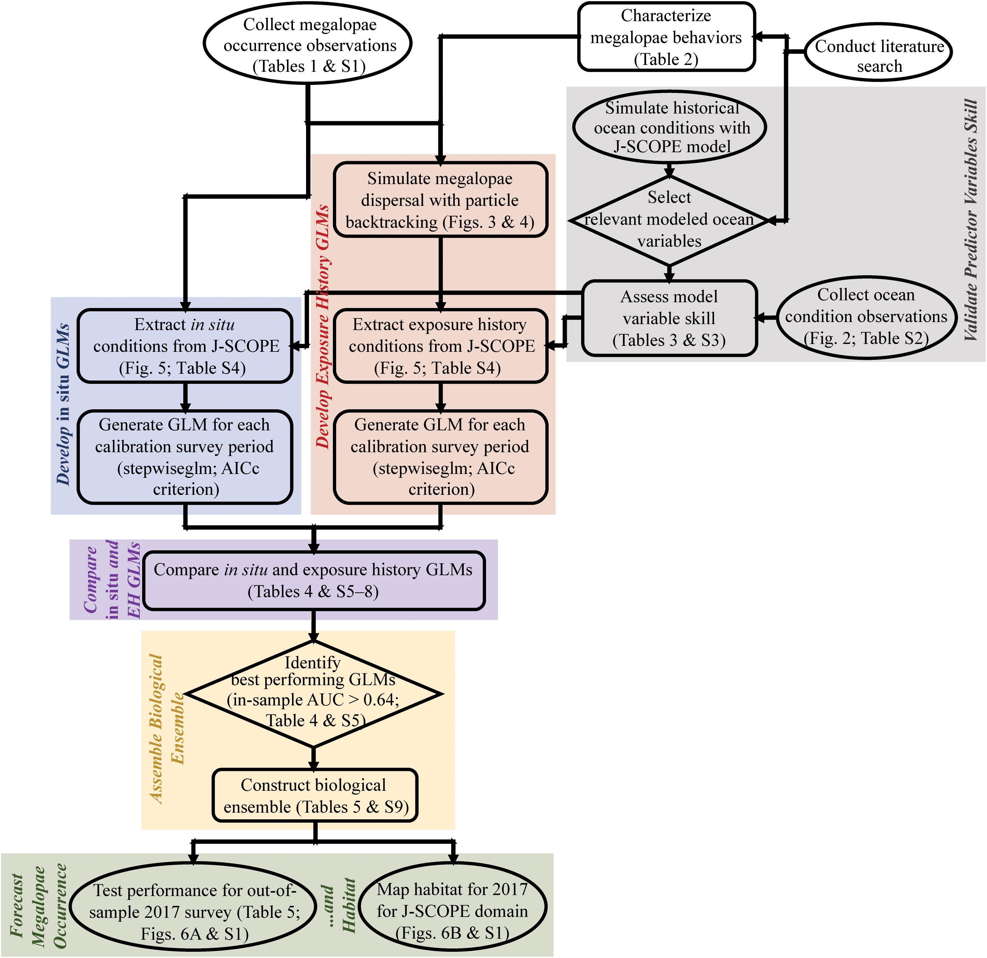
Figure 1. Flowchart summarizing the main methods and results of this paper, including validation of predictor variables skill (gray); development of in situ (blue) and exposure history (red) generalized linear models (GLMs); comparison of in situ and exposure history GLMs (purple); assembly of the biological ensemble (yellow); and forecasting of megalopae occurrence and habitat (green). Start and end nodes are in ovals, process steps are in boxes, and decision points are in diamonds. Table SX refers to Supplementary Tables (1–9). AICc = Akaike information criterion corrected for small sample size; AUC = area under the receiver operating characteristic (ROC) curve; EH = exposure history; GLM = generalized linear model; J-SCOPE = JISAO’s Seasonal Coastal Ocean Prediction of the Ecosystem.

Metacarcinus magister Megalopae Collection

Metacarcinus magister larvae were collected on surveys conducted by NOAA Northwest Fisheries Science Center (NOAA/NWFSC) as part of a larger study of juvenile salmonids and associated nekton (Morgan et al., 2019) at 37 unique stations off of the Washington and Oregon coasts from 2009 to 2017 (Table 1 and Supplementary Table 1). Surveys were conducted during the daytime in late May and/or June for approximately week-long periods. Larvae were collected using a 0.6 m bongo net with 335 μm mesh size. Plankton nets were towed obliquely by letting out 60 m of cable and immediately retrieving it at a rate of 30 m/min while being towed at two knots. Thus, nets were fished from a maximum depth of 20–30 m to the surface, spanning a large portion of the expected depth habitat of megalopae (see details below). Samples were immediately preserved in 5% buffered formalin/seawater solution and returned to the laboratory for analysis. In the laboratory, plankton samples were rinsed and then sorted based on larval developmental stage and enumerated. For more details on field and laboratory methods, see Morgan et al. (2005). For this study, we modeled megalopae occurrence, characterized as presence or absence of megalopae at each sampling station.

TABLE 1

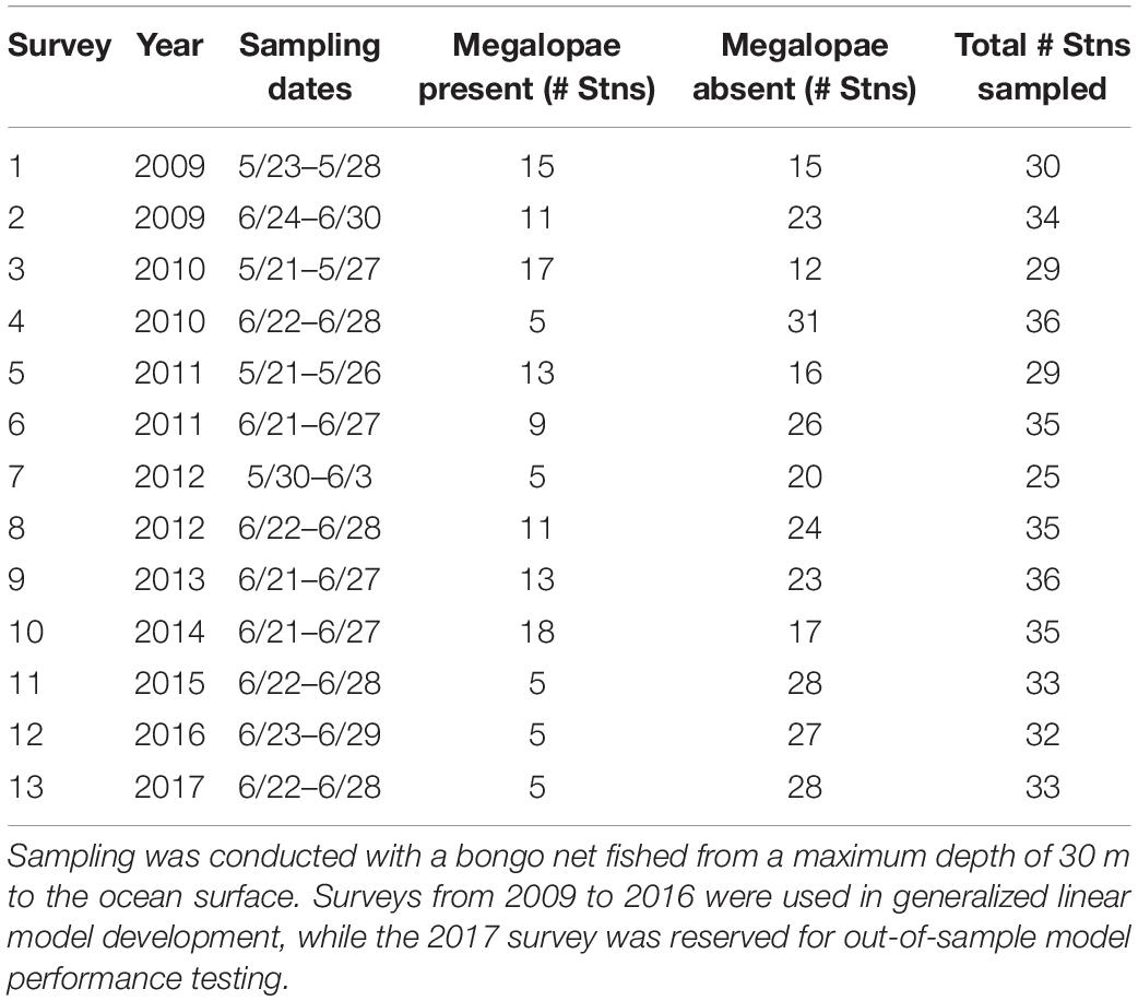
Table 1. Megalopae sampling survey information, including sampling date, number of stations where megalopae were present and absent, and total number of stations sampled (see Figure 4A for map; see Supplementary Table 1 for sampling location information).

Modeled Ocean Conditions

J-SCOPE Historical Ocean Simulations

Historical ocean simulations (i.e. hindcasts) were used in lieu of empirical measurements because they provide spatially and temporally continuous ocean conditions. We have conducted extensive model evaluation with ocean observations for all the variables considered here (see Siedlecki et al., 2016, and results below). Modeled environmental variables, obtained from the J-SCOPE ocean model (Siedlecki et al., 2016), were used to develop the GLMs to predict megalopae occurrence. Environmental conditions were extracted from historical ocean simulations for 2009–2016 corresponding to either the megalopae collection times and locations (in situ GLM) or along backtracking particle trajectories (exposure history GLMs; more details below). Historical ocean simulations for 2017 were reserved for GLM performance testing.

J-SCOPE Variable Skill Assessment

Validation of J-SCOPE’s historical ocean simulations was performed for a wider range of environmental variables than in previous work (e.g. Siedlecki et al., 2015, 2016; Year in Review webpages at http://www.nanoos.org/products/j-scope/). Additionally, assessments were performed for distinct depth intervals (Table 2) to investigate the skill of particular ocean conditions as they were experienced by in situ or exposure history particles, since the skill of these predictor variables may be relevant to the subsequent performance of the megalopae occurrence GLMs. To accomplish this, empirical observations were matched temporally and spatially to modeled variables.

TABLE 2

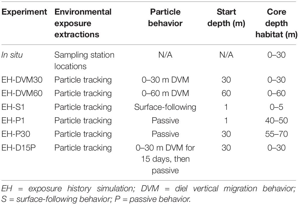
Table 2. Environmental condition extractions for in situ (row 1) and particle tracking (rows 2–7) experiments, including (when relevant) where environmental conditions were extracted, the behavior simulated for particles, the depth at which particles were initialized, and the core depth habitat.

Ocean Observational Data

Observational data were compiled from regional moorings and surveys conducted from 2009 to 2017 (Figure 2 and Supplementary Table 2). CTD-based measurements of temperature, salinity, oxygen, and phytoplankton (measured as fluorescence) were made ∼1–2 times per month from 2009 to 2017 at seven stations across the continental shelf and slope along the Newport Hydrographic Line (NHL; 44.6517°N). Surface nitrate data were also collected along the NHL. NOAA/NWFSC Groundfish bottom trawl surveys measured bottom temperature on the continental shelf and slope from 2009 to 2014. Nitrate was also measured at surface and sub-surface locations during the NOAA/NWFSC Northern California Current survey in 2011. In addition to megalopae sampling conducted by NOAA/NWFSC Juvenile Salmon surveys, nitrate was measured at 3 m depth at 37 stations off the Washington and Oregon coasts from 2009 to 2014. Temperature and oxygen were observed at surface and sub-surface locations ∼1–2 times per month from 2009 to 2017 at the Cape Elizabeth mooring in the Olympic Coast National Marine Sanctuary (OCNMS). Temperature, oxygen, salinity, nutrients (i.e. nitrate, phosphate, and silicate), dissolved inorganic carbon (DIC), and total alkalinity (TA) were measured at surface and sub-surface locations on Pacific Coast Ocean Observing System (PaCOOS) annual surveys in 2009 and 2010. Temperature, oxygen, salinity, nutrients, phytoplankton, DIC, and TA were also measured at surface and sub-surface locations on West Coast Ocean Acidification (WCOA) surveys conducted in 2011, 2012, 2013, and 2016. For all surveys with temperature, salinity, phosphate, silicate, DIC, and TA measurements, values of pH (at in situ temperature, salinity, and pressure, on the total scale) and aragonite (Ω_ar) and calcite saturation states (Ω_ca) were calculated in CO2SYS (Pelletier et al., 2007), using carbonate dissociation constants from Lueker et al. (2000), salinity to boron ratios from Uppström (1974), bisulfate equilibrium constants from Dickson (1990), and the “seacarb” option for fluoride (i.e. Perez and Fraga, 1987 when 33 > T > 10 [°C] and 40 > S > 10 [PSU], otherwise Dickson and Riley, 1979). Additionally, empirical relationships using the proxy variables oxygen and temperature were developed to estimate carbonate chemistry variables for the region encompassed by the model domain based on calibration data sets collected on all WCOA surveys following the methods described in Alin et al. 2012; Eqs. 1–3):

FIGURE 2

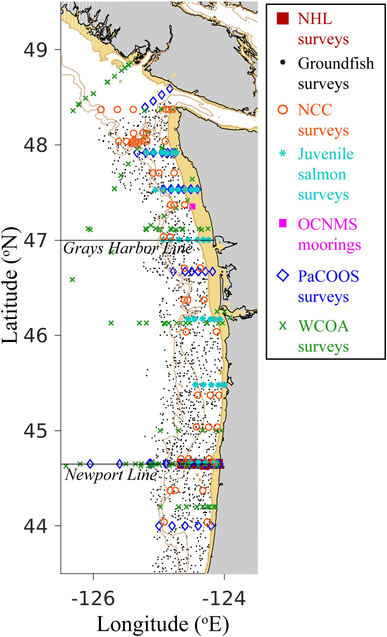
Figure 2. Empirical observation sampling locations used to assess the skill of J-SCOPE modeled ocean variables. Survey and mooring symbols correspond to the figure legend, with tiny black dots representing groundfish survey locations. The Grays Harbor Line and the Newport Line, two common hydrographic transects, are plotted for reference. The 200 and 500 m isobaths are indicated by light brown contours, and depths shallower than 50 m are shaded light brown. Land is shaded gray. NHL = Newport Hydrographic Line; NCC = Northern California Current; OCNMS = Olympic Coast National Marine Sanctuary; PaCOOS = Pacific Coast Ocean Observing System; WCOA = West Coast Ocean Acidification. See Supplementary Table 2 for additional information on sampling dates, depths, and measured parameters.

$$pH=7.2587+0.0021314\times \text{O}+0.018633\times \text{T}(1)$$

$${\text{Ω}}_{ar}=0.990759+0.04372\times \left(\text{T}-T_r\right)+0.0043285\times \left(\text{O}-O_r\right)+0.0006399\times (\text{T}-T_r)\times (\text{O}-O_r)(2)$$

$${\text{Ω}}_{ca}=-20.343+1.8719\times \text{T}+0.0082364\times \text{O}+69.047÷\text{T}-0.046982\times {\text{T}}^2(3)$$

where T_r = 8.1903 and O_r = 144.441 are reference values based on the calibration data set, and T = temperature (°C) and O = oxygen (μmol kg^–1) are modeled or observed values. These equations were applied at sites where both temperature and oxygen data were available. For phytoplankton observations (measured as either fluorescence or chlorophyll), units were converted following the methods of Davis et al. (2014) prior to comparison with the modeled phytoplankton variable (mmol m^–3).

Statistical Skill Calculations

Observations and modeled data were paired within a given depth interval (Table 2), and two statistics were calculated to assess model variable skill: (1) the Pearson correlation coefficient (r), ranging from −1 (negative correlation) to 1 (positive correlation), indicates the degree of linear correlation between the observed and modeled variables; and (2) normalized root-mean-square error (NRMSE) estimates the magnitude of the difference between the observed and modeled variables, with the sign indicating the direction of model bias (positive sign indicates model overestimate; negative sign indicates model underestimate; see Supplementary Equations 1, 2).

Variable Selection for Habitat Models

In situ Variables

To assemble a suite of potential predictor variables for developing the GLM, we selected physical and biogeochemical variables identified in the biological literature as important for the development and survival of M. magister megalopae or a closely related organism, and that exist or can be derived from the J-SCOPE historical ocean simulations. We omitted synthetic or summary variables, such as the PDO or upwelling indices, despite their reported correlations with megalopae abundance (Hobbs et al., 1992; Shanks and Roegner, 2007; Shanks, 2013) because we strive for a mechanistic understanding of how fundamental ocean conditions characterize megalopae habitat—e.g. is it the cooler water temperatures, lower oxygen levels, or more acidified conditions of the upwelled waters that influence habitat? Thus, a total of eight potential predictor variables were considered for inclusion in our statistical models: temperature, salinity, dissolved oxygen concentration, nitrate concentration, phytoplankton concentration, pH, aragonite saturation state (Ω_ar), and calcite saturation state (Ω_ca). Temperature was chosen because it is thought to influence M. magister larval development duration (Moloney et al., 1994; Sulkin and McKeen, 1996; Sulkin et al., 1996) and to be an indicator of advective processes (Ferrari and Ferreira, 2011). Due to the high abundance of M. magister megalopae observed within Columbia River plume fronts, salinity was selected as there is substantial salinity variability within the plume (Morgan et al., 2005), and M. magister larvae are reportedly sensitive to changes in salinity (Pauley et al., 1989). Dissolved oxygen was selected because M. magister megalopae and juveniles experience negative metabolic effects and high mortality rates, respectively, in hypoxic conditions (Bancroft, 2015; Gossner, 2018). In addition to temperature, nitrate concentration is a strong indicator of upwelling, indicating both nutrient sources for primary productivity and offshore Ekman transport (Hales et al., 2005; Palacios et al., 2013). Phytoplankton concentration was selected as an indicator of cross-shelf and alongshore currents and retentive features, and as a proxy for food availability (Largier et al., 2006; Kudela et al., 2008). pH was included because Miller et al. (2016) found that exposure of M. magister larvae to low pH conditions increased mortality and slowed development rates. We selected Ω_ca as a potential predictor because the M. magister megalopae exoskeleton contains calcite (Bednaršek et al., 2020; Boßelmann et al., 2007; Neues et al., 2007). Although Ω_ar may not directly affect the condition of the megalopal exoskeleton, we chose to include this variable as a potential predictor because of the impacts it has on the pelagic food web that may influence megalopae development and survival (Riebesell et al., 2000; Fabry et al., 2008).

Five variables (temperature, salinity, dissolved oxygen concentration, nitrate concentration, and phytoplankton concentration) were extracted directly from the J-SCOPE historical ocean simulations at the stations where megalopae were sampled, and then averaged over the upper 30 m of the water column, the sampling depth of the megalopae collections. The remaining three variables (pH, Ω_ar, Ω_ca) were calculated with empirically derived formulae that used dissolved oxygen concentration and temperature at the station locations from the J-SCOPE historical ocean simulations (see equations above); these were then averaged over the surface 30 m.

Exposure History Variables

Simulated megalopae dispersal

To test our hypothesis that recent environmental exposure history is important in determining megalopae occurrence, we used particle tracking to simulate virtual megalopae dispersal. Since megalopal stage duration is approximately 30 days for temperatures in this region (Poole, 1966; Ebert et al., 1983) and physical uncertainty in the particle trajectories due to unresolved vertical and horizontal advection and diffusion becomes large over approximately the same time span (sensitivity analyses not shown), particles were tracked backward in time for a period limited to 30 days. Future studies may incorporate earlier larval developmental stages (e.g. zoeae) or run full lifecycle individual-based models, but the current study focuses on whether the environmental exposure over the course of the 30 days prior to megalopae collection can be used to improve megalopae occurrence modeling. Thus, we simulated megalopae dispersal with an offline particle tracking model, the Larval TRANSport Lagrangian model (LTRANSv2b; North et al., 2008, 2011; Schlag and North, 2012), driven by external physical forcing, random displacement, and directed swimming behaviors as prescribed by the user. To account for stochasticity, 100 particles were initialized at each of the 37 sampling stations on the last day of each survey (Table 1). Ocean velocities from J-SCOPE hourly historical ocean simulations were “reversed” (i.e. negated) to force particle advection backward in time, and particle behavior was imposed.

Although researchers have used observations of the horizontal and vertical distribution of larvae to infer swimming behavior, these behaviors have not been precisely characterized. Thus, six particle back-tracking experiments were run to simulate the depth habitats occupied and the range of behaviors potentially exhibited by M. magister megalopae in the 30 days prior to collection (Table 2). In the first two simulations, particles exhibited diel vertical migration (DVM) behavior to daytime depths of either 30 m (“EH-DVM30”) or 60 m (“EH-DVM60”), per depth variations reported in the literature (Hobbs and Botsford, 1992). These behaviors simulated active swimming down to the maximum depth at dawn, maintaining that depth throughout the day (∼16 h), swimming up to the water’s surface at dusk, and maintaining the near surface habitat for the remainder of the night (∼8 h; swimming speed = 10 cm/s; Fernandez et al., 1994; Rasmuson, 2013; Rasmuson and Shanks, 2014). In the third simulation, particles sustained a near-surface habitat by constantly swimming upward (“EH-S1”) to mimic anecdotal reports of surface aggregations of megalopae in swarms or attached to flotsam (Lough, 1976; Shenker, 1988). Although DVM and surface-following behaviors are most commonly reported in the biological literature for megalopae, we ran two additional simulations that allowed particles to disperse passively (i.e. no swimming behavior) after being initialized either at the surface (“EH-P1”) or at 30 m depth (“EH-P30”), which represent the vertical limits of the plankton collection tows. Passive behavior was simulated for two reasons: (1) because the collected organisms were identified to developmental stage (i.e. megalopae) but their precise age was unknown, organisms that had recently molted from the last zoeal stage would have exhibited reduced swimming abilities commensurate with the earlier life stage (Jacoby, 1982) for potentially a large portion of the back-tracking period, which would be more closely approximated by passive dispersal; and (2) to investigate the effects of behavior on environmental exposure history, passive dispersal served as a null model for comparison with the active behaviors. The passive dispersal simulations included a backward random walk in the vertical direction, whose magnitude was calculated at each time step based on the stored local value of vertical diffusion calculated by the J-SCOPE historical ocean simulation. Finally, to account for megalopae who may have molted from the final zoeal stage mid-way through the 30-day period prior to collection, we simulated a behavior for which the particle exhibited DVM (0–30 m depth) for the first 15 days of the back-tracking simulation, followed by passive dispersal for the second half of the simulation (“EH-D15P”). For all behaviors, simulated dispersal trajectories were updated every 60 s, and particle locations and ambient environmental conditions were recorded hourly.

Prior to calculating exposure history for the particle tracks, we removed records of particles that had exited the model boundaries, which included particles located in the Columbia River and Salish Sea, due to a lack of confidence in the biogeochemical modeling in those areas (i.e. particles located at longitude > −123.9°E or < −126.5°E or latitude > 49.5°N or < 43.5°N; 12.2% of exposure history records). Additionally, we removed any particle exposure data that had unrealistic negative values due to extrapolation errors when a particle was located either at the ocean surface or just above the seafloor (0.29% of exposure history records).

Exposure history variable calculations

Two types of exposure history statistics were calculated for each particle and then averaged across all particles (N = 100) initialized at each station. (1) Average environmental conditions for all variables (temperature, salinity, dissolved oxygen concentration, nitrate concentration, phytoplankton concentration, pH, Ω_ar, and Ω_ca) were calculated by extracting the ambient environmental field from the J-SCOPE historical ocean simulations along the particle trajectory and then averaging over the entire 30-day simulation. (2) Severity indices (“SI”), which are a combined metric of the intensity and duration of exposure to stressful conditions, were calculated for a subset of environmental variables (oxygen, pH, Ω_ar, and Ω_ca) by multiplying the duration of time (in days) and magnitude beyond an environmental threshold that a particle was exposed to a stressful condition, and then summed over the 30-day backtracking simulation (Hauri et al., 2013; Bednaršek et al., 2017; Supplementary Equations 3, 4). Environmental thresholds for the severity indices were defined as oxygen < 1.4 ml l^–1 (O₂ < 62 mmol m^–3; 61 μmol kg^–1; i.e. hypoxia), pH < 7.75 (Feely et al., 2008, 2016; Hodgson et al., 2016; Miller et al., 2016), Ω_ar < 1 (i.e. physical threshold for aragonite dissolution), and Ω_ca < 1 (i.e. physical threshold for calcite dissolution).

Developing a Habitat Model for Megalopae

GLM Development

A GLM was used to identify the modeled environmental variables that best explain the temporal and spatial heterogeneity in M. magister megalopae occurrence in coastal Washington and Oregon waters. Although life stage processes and population dynamics are assumed to be non-linear, linear models are often used to approximate these processes in fisheries science (e.g. Ricker, 1973; Austin and Cunningham, 1981; Guisan et al., 2002; Venables and Dichmont, 2004), and GLMs have been used successfully to predict probability of occurrence for a wide range of species (Brotons et al., 2004; MacLeod et al., 2008; Krigsman et al., 2012; Froehlich et al., 2015). A GLM is a statistical model that relates a combination of predictor variables (i.e., modeled ocean variables) to a response variable (i.e. megalopae occurrence characterized as presence or absence at each sampling station). Because our response variable had a binomial distribution (i.e. megalopae were either “present” or “absent”), we used a logit link function (Eq. 4; Fisher, 1954),

$$f(\mathrm{\mu })=log\left(\frac{\mathrm{\mu }}{1-\mathrm{\mu }}\right)(4)$$

where

$$\mathrm{\mu }=\frac{e^{X_b}}{1+e^{X_b}}(5)$$

where X_b is a linear combination of predictor variables (Eq. 5).

To examine the hypothesis that exposure history is an important driver of megalopae occurrence, a suite of potential GLMs were developed using environmental variables from one of two types of experiments (Table 2): (1) “in situ” ocean conditions extracted from the model at the times and locations where megalopae were sampled; and (2) exposure history statistics for ocean conditions were extracted along particle trajectories from six distinct particle behavior simulations. We included modeled variables from all 12 surveys (2009–2016; i.e. the “calibration survey period”) during GLM development. The automated GLM forward and backward stepwise function in Matlab (R2018b; stepwiseglm) was used to evaluate all possible combinations of the suite of predictor variables (eight variables for the in situ models; 12 variables for the exposure history models), and to add and/or remove variables until the best GLM with the lowest Akaike information criterion corrected (AICc) score for small sample size was derived (Burnham and Anderson, 2002). Non-significant and/or potentially collinear predictors were retained in GLMs if their removal resulted in an increased AICc score, indicating that they contributed to model fit despite their lack of statistical significance and/or independence from other predictors in the model. AICc scores attempt to balance the inclusion of additional predictor variables that improve model fit but result in increased model complexity by imposing a penalty for variable inclusion to prevent over-fitting and subsequent declines in model prediction performance (Wilks, 1995). AICc scores were used to compare GLMs developed using in situ and exposure history experiments.

To investigate the impacts of year effects due to inter-annual variation in environmental conditions in the northeast Pacific Ocean (e.g. El Nino-Southern Oscillation and an anomalous “marine heatwave” in 2014–2016; Bond et al., 2015; Fisher et al., 2015; Thompson et al., 2018) and variability in J-SCOPE model skill (e.g. Year in Review pages at http://www.nanoos.org/products/j-scope/) on GLM model development, we conducted a modified sliding window analysis to develop additional GLMs. Here, we modified the calibration survey period to include only 10 of the 12 surveys available between 2009 and 2016 during GLM development, i.e. all combinations of 10 out of 12 surveys [mathematically, C(12,10)] were used to develop an additional 66 GLMs for the in situ and exposure history experiments, following the methods described above.

Biological Ensemble Assembly

Since the primary aim of this study was to generate the best model for forecasting inter-annual megalopae occurrence patterns, we relied on a model performance metric, the in-sample AUC value, to identify high-performance GLMs across experiments (i.e. in situ or exposure history behaviors). The in-sample AUC value [“area under the receiver operating characteristic (ROC) curve,” see Fielding and Bell, 1997] measures model performance on the data used to develop the model. AUC is calculated by comparing the GLM output probability to the observed presence/absence for megalopae at each station. AUC ranges from 0 to 1, with AUC < 0.5 indicating no model skill, and 0.5 < AUC ≤ 1 indicating skill above random chance.

Due to the high performance of several individual GLMs across exposure history experiments, we selected multiple GLMs to form a “biological ensemble” to represent a range of simulated megalopae behaviors for forecasting applications (see below). We used a criterion of in-sample AUC ≥ 0.64 to identify a cluster of top-performing GLMs to include in the biological ensemble. Each member GLM was weighted equally. To evaluate potential collinearity of variables in the final biological ensemble, correlation coefficients were calculated for predictor variables in each member GLM.

Applying the Habitat Model

Biological Ensemble Performance Evaluation

To quantify the biological ensemble’s ability to forecast megalopae occurrence, the ensemble was used to predict megalopae occurrence for the out-of-sample 2017 survey. Each member GLM of the biological ensemble was individually evaluated for 2017, and then the forecasted megalopae occurrence probabilities were averaged across the member GLMs to obtain the biological ensemble forecast for 2017. Specifically, particle simulations using J-SCOPE modeled ocean conditions for 2017 were conducted for each behavior represented by the GLMs in the biological ensemble. Exposure histories for each behavior were incorporated into the relevant member GLM to generate five independent forecasts of megalopae occurrence probabilities for each sampling site. These five sets of probabilities were then averaged (with equal weighting of each member GLM) to forecast megalopae occurrence probabilities for the biological ensemble as a whole. Ultimately, an AUC value was calculated by comparing the biological ensemble’s forecasted megalopae probabilities to megalopae occurrence observed on the 2017 survey.

Habitat Forecasting

Finally, megalopae habitat throughout the J-SCOPE model domain was forecast for 2017 using the biological ensemble. Habitat prediction simulations were run for each behavior represented by the GLMs in the biological ensemble, using particles initialized over a grid throughout the x/y domain of the J-SCOPE ocean model. As described above, the particle exposure histories were incorporated into the individual GLMs comprising the ensemble, and then those output probabilities of megalopae occurrence were averaged across the member GLMs to generate a spatially comprehensive forecast of megalopae habitat for the biological ensemble for 2017.

Results

Generalized linear models predicting megalopae occurrence based on the experiments outlined in Table 2 were constructed using modeled ocean conditions from either in situ megalopae sampling locations or exposure history simulations based on particle tracking experiments with unique behavior and initialization depth. Comparing these GLMs allowed us to investigate the hypothesis that exposure history is important for characterizing megalopae occurrence. Because these GLMs are built from modeled ocean variables, we begin by reporting skill assessments for these variables to understand their influence on GLM fit and performance.

J-SCOPE Variable Skill Assessment

Environmental variables from J-SCOPE historical ocean simulations performed well (as indicated by r and NRMSE; Table 3) within the depth habitats dictated by the simulated megalopae behaviors (Table 2) and during the time period when particle dispersal was simulated (May–June). All but one of the variables (phytoplankton) had a significant correlation with the observations at all depth habitats (r > 0.5), and variable performance generally improved with depth. Phytoplankton did not perform as well as the other variables, except near the ocean surface (0–5 m). Year-round model validation showed similar patterns as seen in the May–June validations (Supplementary Table 3).

TABLE 3

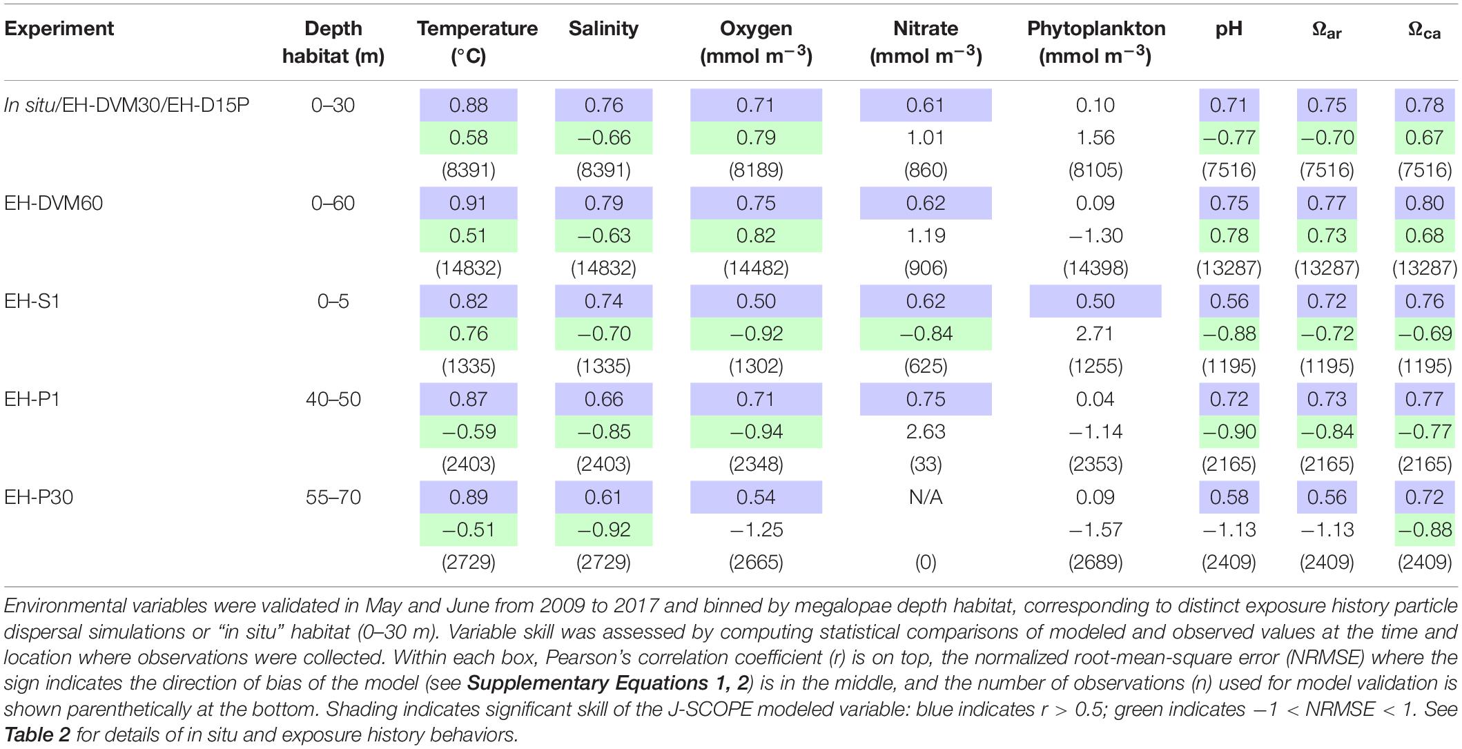
Table 3. Skill assessment of J-SCOPE historical ocean simulation variables that will be considered as potential predictor variables during megalopae occurrence GLM development.

Environmental Exposure of Megalopae

The exposure histories generated by the particle tracking experiments were driven predominantly by the particle depth habitats, which were determined by particle behavior and initialization depth (Figures 3–5; ANOVA results shown in Supplementary Table 4). On average, particles exhibiting passive dispersal initialized at 30 m depth (EH-P30) inhabited significantly deeper waters (mean particle depth = 47.1 ± 13.3 m (mean ± std); Figure 3 and Supplementary Table 4) and originated farther offshore (mean particle ending isobath = 572 ± 455 m; Figure 4) than particles in any other experiment. The properties of the simulated ocean conditions that these particles were exposed to were ultimately different because of their unique depth habitat (Figure 5 and Supplementary Table 4). Exposure histories for these passive particles were characterized by significantly lower temperature, dissolved oxygen concentration, phytoplankton concentration, pH, Ω_ar, and Ω_ca, and significantly higher salinity and nitrate concentrations than particles in other exposure history simulations. Consequently, particles in this experiment were exposed to the most severe hypoxic stress and corrosive waters [severity index (SI) for oxygen = 2.14 ± 3.23 hypoxia-days; SI pH = 1.88 ± 1.45 days with pH < 7.75; SI Ω_ar = 2.90 ± 2.37 undersaturation-days; SI Ω_ca = 1.69 ± 2.13 undersaturation-days). In contrast, the surface-following particles (EH-S1) had a tightly constrained depth habitat within ∼5 m of the ocean surface (mean particle depth = 2.39 ± 0.04 m), which was significantly shallower than any of the other experiments (Figure 3). Their exposure histories were characterized by significantly higher temperature, oxygen, phytoplankton, pH, Ω_ar, and Ω_ca, and significantly lower salinity and nitrate concentrations (Figure 5 and Supplementary Table 4). Thus, these surface-following particles experienced minimal exposure to hypoxic and corrosive waters (SI Oxygen = 0.02 ± 0.06 hypoxia-days; SI pH = 0.07 ± 0.15 days below 7.75 pH; SI Ω_ar = 0.10 ± 0.20 undersaturation-days; SI Ω_ca = 0.002 ± 0.004 undersaturation-days). Particles in other experiments were exposed to intermediate environmental conditions at intermediate depth habitats. Passive particles initialized at the surface (EH-P1; mean particle depth = 20.4 ± 20.7 m) had exposure histories most similar to particles in the 30 m DVM experiment (EH-DVM30; mean particle depth = 20.3 ± 1.2 m) and the experiment where particles transitioned from DVM to passive dispersal (EH-D15P; mean particle depth = 20.7 ± 7.3 m). Passive dispersal particles initialized at 30 m (EH-P30; mean particle depth = 47.1 ± 13.3 m) experienced conditions most similar to the 60 m DVM particles (EH-DVM60; mean particle depth = 30.8 ± 2.4 m). In situ extracted conditions were most similar to those experienced by passively dispersing particles initialized at the surface (EH-P1).

FIGURE 3

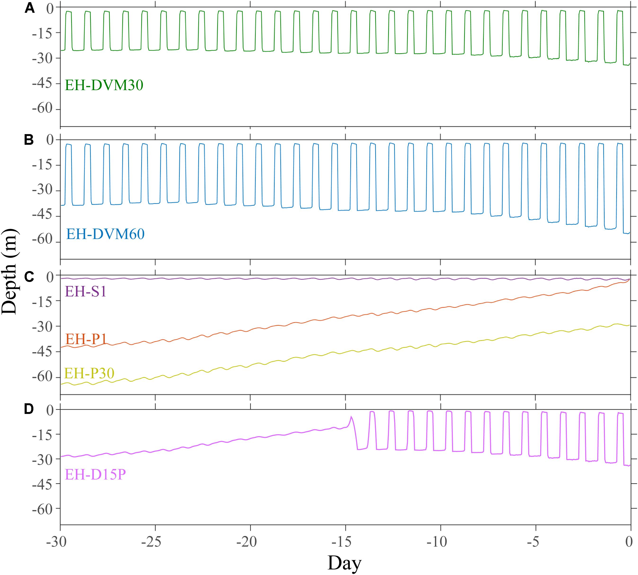
Figure 3. Average depth and variability over time was driven by simulated particle behavior and initialization depth. Particles exhibiting DVM behaviors were tightly constrained between 30 m (EH-DVM30; A) or 60 m depths (EH-DVM60; B) and the surface. (C) Passive particles initialized at 1 m (EH-P1) and at 30 m depths (EH-P30) originated from deeper depths and traveled up in the water column over time, while surface-following particles (EH-S1) experienced a tightly constrained depth habitat near the surface. (D) These particles spent the first 15 days of the simulation exhibiting DVM between the surface and 30 m depth, and then they transitioned to passive dispersal (EH-D15P).

FIGURE 4

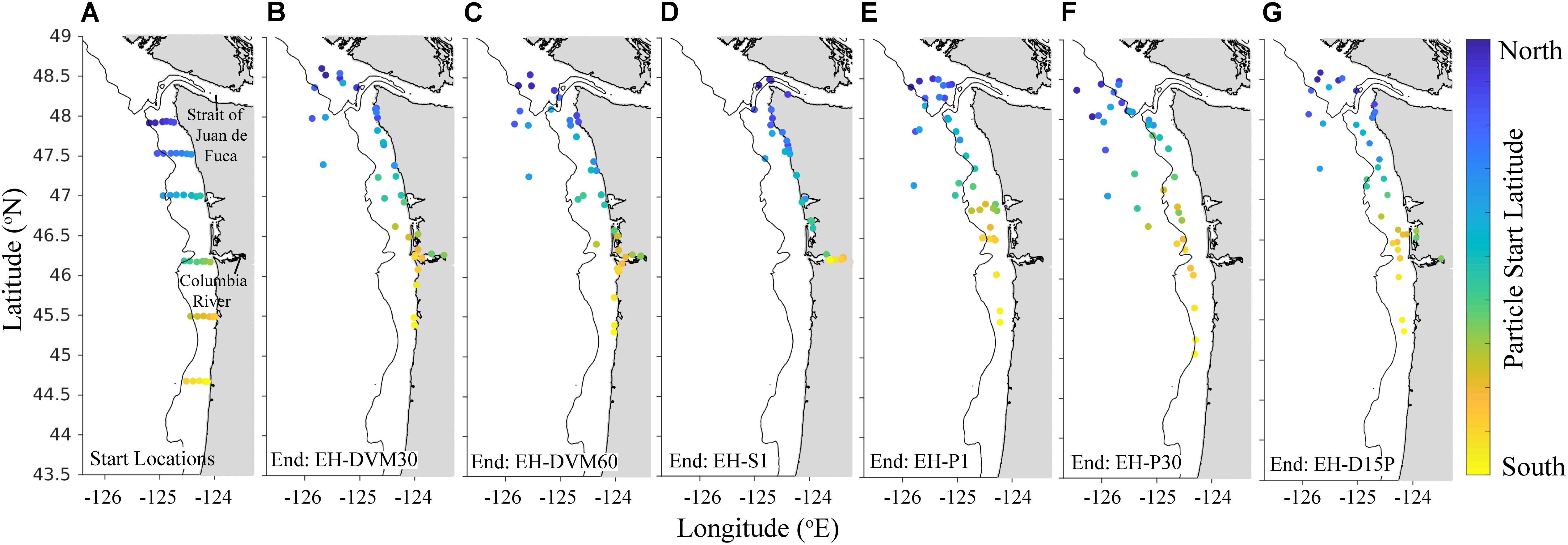
Figure 4. Particle start (A) and average back-tracked origination locations (B–G) after 30-day simulated backtracking for particle exposure history simulations (2009–2017) that varied by behavior and initialization depth: DVM behavior from the surface to 30 m (EH-DVM30; B) and 60 m depths (EH-DVM60; C); the surface-following behavior (EH-S1; D); passive particles initialized at 1 m (EH-P1; E) and at 30 m depths (EH-P30; F); and DVM transitioning to passive dispersal at day 15 (EH-D15P; G; see Table 2 for details about exposure history experiments). Particles were initialized at the same 37 sampling stations. Back-tracked origination locations were averaged for all 100 particles initialized at each station, which sometimes resulted in the average origination location being on land; these particles were moved to the nearest shoreline. Initialization locations are uniquely colored for improved resolution of differing dispersal patterns across the spatial domain. Land is shaded gray, and the 200 m isobath is shown for reference.

FIGURE 5

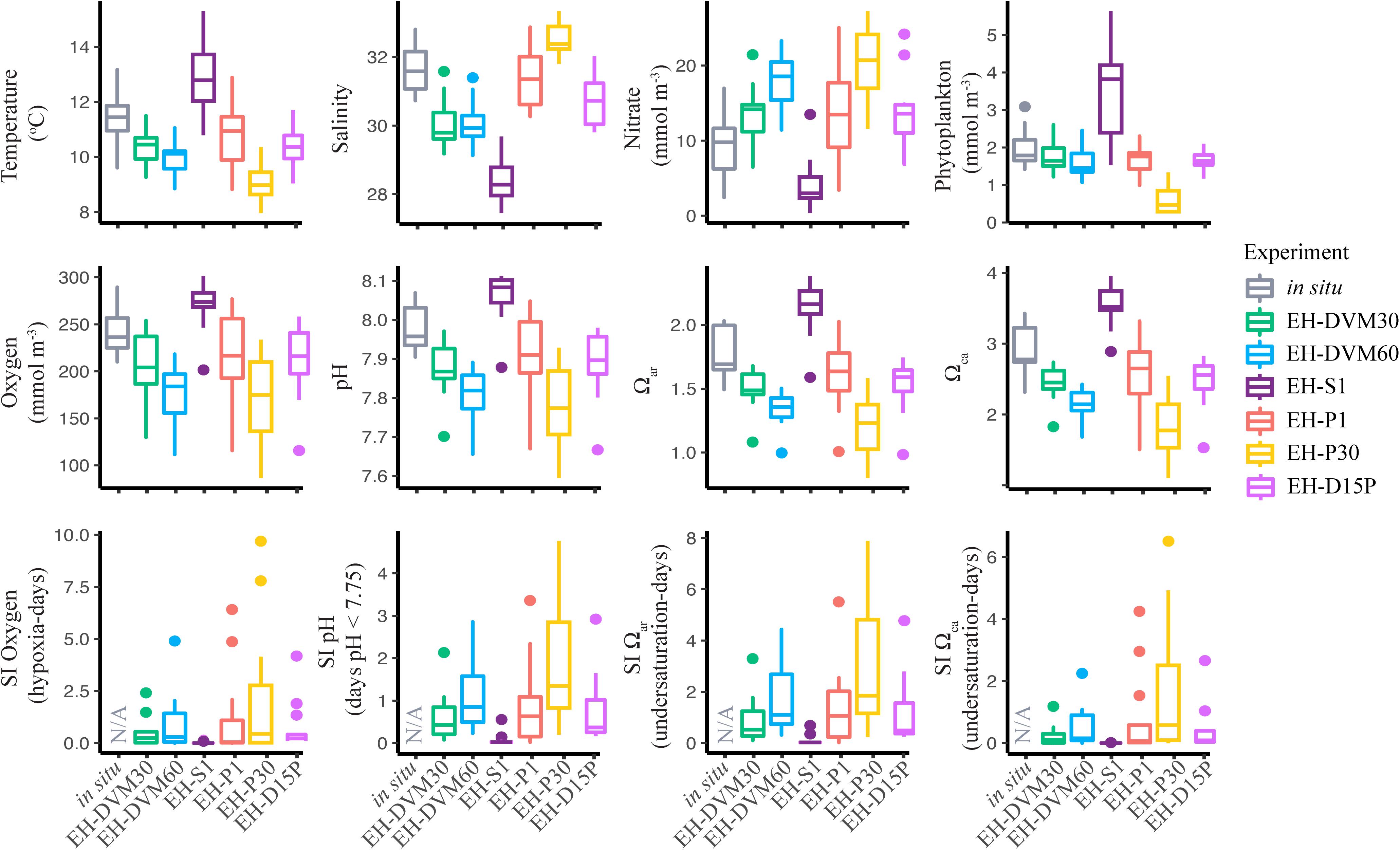
Figure 5. In situ conditions and particle tracking exposure histories differed among years and among simulations with different particle behaviors and initialization depths. These box and whisker plots show the interquartile range (bounds of the box) with a horizontal line at the median, ends of the vertical lines at the fifth and 95th percentiles, and outliers represented by dots. Averages were calculated across all particles within an in situ extraction or particle tracking simulation, and statistics were calculated across survey averages to show variability over time (2009–2017; see Supplementary Table 4 for ANOVA results).

GLM Comparisons: In situ Versus Exposure History

Inclusion of environmental exposure history during GLM development improved our ability to predict megalopae occurrence. The in situ GLM had the worst model fit (i.e. highest AICc score) and worst in-sample model performance (i.e. lowest AUC) compared to the exposure history models (Table 4; see additional statistics in Supplementary Table 5). Sliding window analyses that were used to evaluate the influence of individual surveys on GLM fit and performance (Supplementary Table 6) provided further support that, independent of the calibration survey period used to develop the GLM, the in situ model was out-performed by the exposure history models in 65 out of 66 cases (98% of cases).

TABLE 4

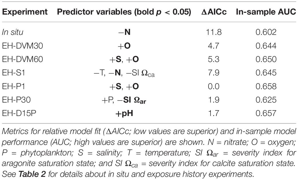
Table 4. Predictor variables [significant predictors in bold (p < 0.05)] and their direction of correlation to megalopae occurrence for generalized linear models (GLMs) developed using surveys from 2009 to 2016 (see Supplementary Table 5 for additional statistics and Supplementary Tables 6, 7 for results from the sliding window analysis).

Among the exposure history GLMs, model fit and in-sample performance were affected by the type of simulated behavior and the depth at which the particles were initialized (Table 4 and Supplementary Table 6). Simulations that included passive dispersal (EH-P1, EH-D15P, and EH-P30) had the best model fit (i.e. lowest AICc scores), followed by DVM behaviors (EH-DVM30 and EH-DVM60), and then the surface-following behavior (EH-S1). These rankings of model fit based on simulated behavior were supported by the sliding window analyses as well (Supplementary Table 6). In-sample model performance, however, showed a different pattern of GLM rankings. When all surveys from 2009 to 2016 were used for GLM development, in-sample AUC indicated highest model performance for the EH-P1 GLM, followed by EH-D15P, EH-DVM60, EH-S1, EH-DVM30, and finally EH-P30 GLMs (Table 4). The sliding window analysis showed similar results, such that the EH-P1, EH-D15P, and EH-DVM60 GLMs generally had the highest performance, but on average, the EH-DVM30 and EH-P30 GLMs performed better than the EH-S1 GLMs (Supplementary Tables 6, 7).

The GLMs contained different significant predictors depending on whether or not exposure history was included, and which particle tracking behavior was simulated (Table 4). The predictors included in the GLMs calibrated with all surveys from 2009 to 2016 were oxygen (three occurrences), salinity (two), nitrate (two), SI for Ω_ca (one), phytoplankton (one), SI for Ω_ar (one), temperature (one), and pH (one). Although the sliding window analysis indicated that the calibration survey period used to develop the GLM had some influence on which predictors were included in the GLMs (Supplementary Tables 6, 8), the relative frequency of the most common predictors was similar to that observed in the GLMs developed using all surveys: oxygen (194 occurrences), salinity (161), nitrate (146), Ω_ca (76), SI for Ω_ca (66), phytoplankton (60), Ω_ar (38), SI for Ω_ar (36), and temperature (35; Supplementary Table 8).

Biological Ensemble Formation

Due to the overall high performance of several GLMs and slight variations in their relative performance when different calibration survey periods were used (Supplementary Table 6), we decided to select multiple models to generate a biological ensemble that we expect to be more robust to interannual variability than any single model (Table 5). The biological ensemble is comprised of five GLMs with the highest overall in-sample model performance (i.e. AUC ≥ 0.64) from the following exposure history behaviors: 30 m DVM (EH-DVM30), 60 m DVM (EH-DVM60), surface-following (EH-S1), passive dispersal initialized at 1 m depth (EH-P1), and DVM transitioning to passive dispersal (EH-D15P). For the biological ensemble, megalopae abundance was positively correlated with salinity, oxygen, and pH, and negatively correlated with temperature, nitrate, and the SI for Ω_ca. Correlation coefficients calculated for pairwise comparisons of predictor variables within a single GLM indicated low dependency among variables (Supplementary Table 9).

TABLE 5

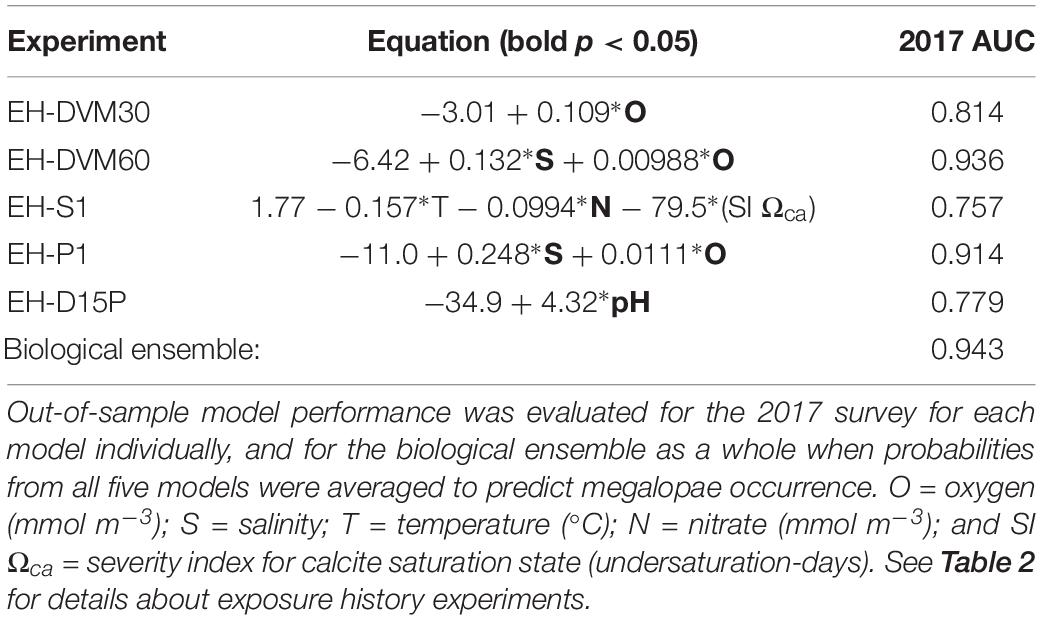
Table 5. A biological ensemble of GLMs [significant predictors in bold (p < 0.05)] assembled from models with strong in-sample performance (AUC (2009–2016) ≥ 0.64; see Table 4 for all models considered).

Habitat Model Performance and Predictions

When model performance was tested for the biological ensemble using the out-of-sample 2017 survey, the ensemble performed better than random (AUC > 0.5), indicating skill in predicting megalopae occurrence (Table 5). Each member of the biological ensemble performed better than random (AUC > 0.5; Supplementary Figure 1), and the ensemble as a whole performed better than any individual member (AUC = 0.94). An AUC value of 0.94 means that for 94% of the stations where megalopae were found to be present, the model predicted a higher probability of megalopae occurrence than for randomly sampled stations where megalopae were observed to be absent.

Finally, when we simulated dispersal of megalopae initialized throughout the J-SCOPE model domain, and applied their environmental exposure histories within the biological ensemble, we were able to generate a spatially explicit habitat model for Washington and Oregon (Figure 6). Over this larger domain, the biological ensemble predicted relatively high probabilities of megalopae occurrence seaward of the continental shelf break. Additionally, megalopae occurrence probabilities tended to increase with latitude. Markedly low probabilities of megalopae occurrence were predicted near the mouth of the Columbia River and near the Strait of Juan de Fuca.

FIGURE 6

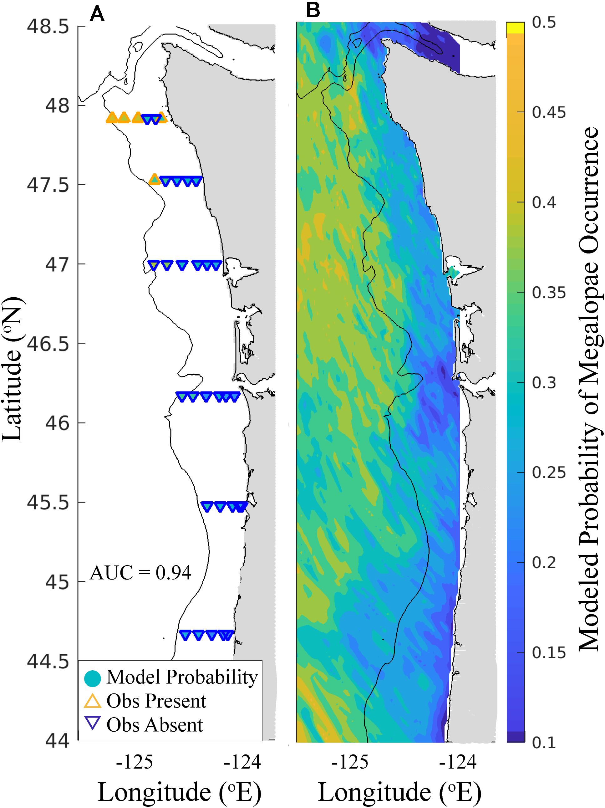
Figure 6. Biological ensemble model forecast for the out-of-sample 2017 survey. (A) Comparison of ensemble-predicted and observed megalopae occurrence at 33 stations. Markers located at the megalopae sampling stations are filled (see color bar) according to the probability of megalopae occurrence as predicted by the biological ensemble (see Table 5). The outline color and orientation of the triangle indicates whether megalopae were observed to be present (orange, upward-pointing triangles) or absent (blue, downward-pointing triangles) at that station. (B) Probability of megalopae occurrence throughout the J-SCOPE x, y model domain forecasted by the biological ensemble (see color bar). Land is shaded gray, and the 200 m isobath is shown.

Discussion

Importance of Exposure History

Model fit and performance (indicated by AICc and AUC, respectively) improved when megalopae exposure history was used to develop the GLM compared to the in situ GLM, regardless of the type of particle behavior used to simulate megalopae dispersal. This suggests that prior environmental exposure is important to include in addition to in situ conditions when predicting megalopae occurrence. While behavior affected the exposure history of the particles, the type of behavior did not influence the GLM performance as much as the decision to include exposure history itself. A biological ensemble of five top performing exposure history GLMs was created to capture the range of behaviors that best predicted megalopae occurrence. Within the biological ensemble, megalopae occurrence was positively correlated with dissolved oxygen concentration, salinity, and pH, and negatively correlated with temperature, nitrate concentration, and the SI for Ω_ca. These predictor variables suggest that megalopae are less common in nutrient-rich environments, potentially generated by upwelling of deep waters that are corrosive and hypoxic, or inflow from terrestrial sources, such as the Columbia River or the Strait of Juan de Fuca, characterized by warmer temperatures and low salinities (Fiedler and Laurs, 1990; Davis et al., 2014).

Below, we discuss in more detail (1) why a biological ensemble was assembled to encompass the range of potential behaviors exhibited by M. magister megalopae, (2) how the predictor variables in the biological ensemble generate a picture of the preferred habitat for M. magister megalopae, and (3) what the limitations of this work are and how they can be addressed in future studies.

Multiple Behaviors in the Biological Ensemble

The biological ensemble consists of the top performing GLMs which represent the breadth of possible behaviors that forecast megalopae occurrence most skillfully (Table 5). Due to the uncertainty of the precise age of the megalopae at collection, potential life history changes over the 30 days prior to collection may explain why passive, DVM, and surface-following behavior models produced GLMs with strong model fit and performance (Tables 4, 5). M. magister larvae may spend as few as ∼7 days or as many as ∼33 days in the megalopal stage (Poole, 1966; Ebert et al., 1983; Sulkin et al., 1996), so our 30-day backtracking experiments may have spanned a period when larvae had reduced swimming abilities as zoeae (Jacoby, 1982), or our DVM behaviors may have overestimated their swimming speeds (Hobbs and Botsford, 1992). Including a GLM with a combination of passive and DVM behavior (EH-D15P) only increased the performance of the ensemble as a whole. Additionally, the surface-following model (EH-S1) may have simulated reported phenomena of megalopae attaching to flotsam or forming swarms near the water’s surface during the daytime (Lough, 1976; Shenker, 1988; Roegner et al., 2003). Thus, we hypothesize that realistic megalopae behaviors may be more accurately represented through a combination of passive, DVM, and surface-following simulations compared to any one behavior alone.

Modeled Megalopae Habitat Conditions

The biological ensemble, when used to forecast megalopae habitat for the entire J-SCOPE domain and compared to the out-of-sample 2017 survey, performed very well (Table 5 and Figure 6). This spatially explicit model showed increasing probabilities of megalopae occurrence seaward of the continental shelf break. This modeled habitat pattern aligns with reports from the literature that M. magister larvae disperse offshore during early development before traveling back to the continental shelf to settle (Johnson et al., 1986; Pauley et al., 1989; Hobbs et al., 1992; Morgan and Fisher, 2010). On regional scales, low probabilities for megalopae occurrence were predicted near the mouth of the Columbia River, in the Strait of Juan de Fuca, and for near-shore areas in Oregon. Finally, high variability in megalopae occurrence was predicted on kilometer scales. The predictor variables identified in the biological ensemble may provide insight into the environmental conditions that create suitable (and unsuitable) habitat for M. magister megalopae.

The biological ensemble member GLMs can be divided into two depth habitat groups characterized by unique predictor variables. Four of the five models in the biological ensemble were defined by megalopae swimming behaviors that resulted in intermediate depth habitats, in which a small portion of dispersal time was spent at the ocean surface and the majority of time was spent at depth (EH-DVM30, EH-DVM60, EH-P1, and EH-D15P; Tables 2, 5 and Figure 3). In these GLMs, megalopae occurrence was positively correlated with oxygen concentration and/or salinity, or pH. These predictor variables may indicate that megalopae in mid-water depth habitats are sensitive to low oxygen or low pH conditions characteristic of upwelled waters and/or low salinities indicative of terrestrial sources, such as the Columbia River plume or the Strait of Juan de Fuca waters. Preferences for environments characterized by high oxygen, pH, and salinity are generally consistent with the habitat requirements for M. magister described in the literature (e.g. Reed, 1969; Sulkin and McKeen, 1989; Brown and Terwilliger, 1999; Curtis and McGaw, 2012; Descoteaux, 2014; Miller et al., 2016; Gossner, 2018). For example, negative impacts, such as increased mortality, decreased growth, and increased respiration rates, have been demonstrated when M. magister megalopae and juveniles are exposed to hypoxic conditions (Bancroft, 2015; Gossner, 2018). Prior laboratory experiments have also shown increased mortality of M. magister zoeae and megalopae when exposed to low salinity conditions (Reed, 1969; Brown and Terwilliger, 1999), and avoidance of adult crabs to low salinity conditions, except when starved (Curtis and McGaw, 2012). The positive correlation between pH and megalopae occurrence is consistent with reports that M. magister larvae are negatively impacted by exposure to low pH (Descoteaux, 2014; Miller et al., 2016).

In contrast to the intermediate depth habitat models discussed above, the fourth member GLM of the biological ensemble corresponds to megalopae occurrence in near-surface habitats (i.e. the surface-following behavior model, EH-S1). In surface waters, where oxygen concentrations and salinity are relatively consistent across temporal and spatial domains (Figure 5), alternative predictors were identified to characterize preferred habitat, such as minimal exposure to calcite-undersaturated conditions, relatively cool temperatures, and low nutrient concentrations (Table 5). These habitat preferences again may signal avoidance of upwelled waters, characterized by low Ω_ca and rich in nutrients, or terrestrial inputs, with warm temperatures and high nutrient concentrations. The negative correlation between SI for Ω_ca and megalopae occurrence is supported by recent work by Bednaršek et al. (2020) which showed that M. magister megalopae may experience external carapace dissolution due to prolonged exposure to more severe calcite saturation state gradients. Several studies have also highlighted the importance of temperature on larval development and survival in M. magister (Sulkin and McKeen, 1989; Sulkin and McKeen, 1996; Sulkin et al., 1996; Brown and Terwilliger, 1999), and our results indicate a preference for relatively cool temperatures in shallow habitats where thermal stress may be more common than at depth (Figure 5). If megalopae occurrence is linked to exposure history via a mortality mechanism, then our results may suggest that megalopae experience lethal temperatures in shallow habitats over the 30-day particle tracking simulations. To our knowledge, no studies have investigated the direct effects of nitrate concentrations on megalopae survival or development. We propose that low nutrient concentrations may indirectly define megalopae habitat by serving as a proxy for preferred downwelling regimes (Hales et al., 2005; Palacios et al., 2013) outside of freshwater plumes, or may indicate the presence of food sources (such as phytoplankton and zooplankton), causing a draw-down of nutrients.

A novel approach taken by this study was to evaluate the skill of modeled variables within the specific depth range and season relevant to our study species. Since the skill of the ocean variables influences the skill of the GLMs to predict megalopae occurrence, and ultimately to model preferred habitat, differences in variable skill may help explain differences in predictive power of GLMs developed with exposure histories from unique behavior simulations. Overall, our model validation showed that ocean variable skill generally improved with depth (Table 3), consistent with prior work by Siedlecki et al. (2016), but variables with strong skill in surface waters also generated GLMs capable of good model performance (e.g. EH-S1 GLM in Table 5). Notably, the 0–30 m DVM exposure history experiment (EH-DVM30), the DVM transitioning to passive behavior (EH-D15P), and the in situ model all used ocean variables within ∼0–30 m depth range, and thus the J-SCOPE variable skill was similar for all GLMs, yet both exposure history GLMs had better fit (lower AICc) and higher predictive skill (higher AUC) than the in situ GLMs (Table 4 and Supplementary Tables 6, 7). This finding further supports our conclusion that exposure to recent environmental conditions is important to include in modeling megalopae occurrence.

Model Limitations and Future Work

In this study, the suite of potential predictor variables was limited to (1) variables that were included in the J-SCOPE historical ocean simulations, (2) variables whose skill could be assessed using observational data, and (3) variables, or threshold values for severity indices, identified in the published literature as being important for M. magister megalopae or related species. For example, only microzooplankton concentration is modeled in J-SCOPE, a class of zooplankton which is not the main food source for brachyuran crab larvae (Bigford, 1977; Harms and Seeger, 1989; Sulkin et al., 1998; Casper, 2013), so we omitted this variable from consideration. Regarding the severity indices, we used thresholds to characterize stressful conditions that may not be biologically relevant for M. magister megalopae, due to limited availability of published scientific studies (see discussions in Hettinger et al., 2012; Waldbusser et al., 2015). Given the importance of temperature and salinity on modeling megalopae occurrence, severity indices for these conditions could also be developed if critical thresholds were identified.

Here, we assembled the five best-performing GLMs into a biological ensemble with equal weighting of its members, due to a lack of information about realistic larval behaviors in wild populations. Future in situ behavioral studies of M. magister late-stage zoeae and early-stage megalopae would help shape realistic larval behavior in particle tracking simulations and inform the relative weighting of member GLMs in the biological ensemble.

Application of the biological ensemble for modeling megalopae habitat is best applied during the temporal and spatial window of the megalopae observations used in this study—namely, late May (2009–2012) and late June (2009–2017) over the continental shelves of Washington and Oregon. Since marine conditions typically become more stressful as the upwelling season evolves, beginning in ∼mid-April (Austin and Barth, 2002; Hales et al., 2006; Hauri et al., 2015), our model may weight exposure to more stressful conditions more heavily given the relative under-representation of the earlier (May) sampling period in recent years. Additionally, because all megalopae sampling stations were located over the continental shelf, but we applied the biological ensemble to forecast habitat over the entire J-SCOPE model domain, evaluation of the model’s prediction of high-quality megalopae habitat in offshore areas would be essential to utilizing the predicted habitat fields offshore.

Finally, this study laid the groundwork for future forecasting of megalopae abundance. To model more complex dynamics, such as abundance, we will apply either generalized linear mixed models (GLMMs), delta-GLMs, or generalized additive models (GAMs), which have relaxed constraints on the types of relationships allowed between the predictor and response variables (Guisan et al., 2002; Venables and Dichmont, 2004; Brodie et al., 2019). Additionally, we will rely on J-SCOPE seasonal forecasts to predict megalopae abundance on seasonal timescales. Since megalopae abundance is correlated with recruitment into the M. magister fishery 4 years later (Shanks and Roegner, 2007; Shanks et al., 2010; Shanks, 2013), improved forecasts of megalopae abundance, generated without arduous field sampling, would extend the management time horizon from seasonal to more than 4 years in advance, potentially promoting increased long-term planning and stability in the fishery (Hobday et al., 2016; Tommasi et al., 2017).

Conclusion

Inclusion of environmental exposure history improved our ability to predict megalopae occurrence. Ultimately, a biological ensemble was generated from GLMs developed with multiple behaviors to encompass biologically relevant variations in megalopae dispersal. This biological ensemble showed superior predictive performance (high AUC) relative to individual GLMs. The biological ensemble identified positive correlations between megalopae occurrence and oxygen concentration, salinity, and pH, and negative correlations with temperature, nitrate concentration, and the SI for Ω_ca. When considered together, these variables indicate that megalopae habitat is characterized by downwelling conditions seaward of terrestrial inputs, such as Columbia River plume or the Strait of Juan de Fuca waters.

Data Availability Statement

The datasets analyzed in this study are included in this article, in the Supplementary Material, or can be found online (see Supplementary Table 2).

Author Contributions

EN was the principal author of the manuscript, designed and performed backtracking experiments with guidance from SS and AH and conducted habitat modeling with input from SS, IK, and CS. Model skill was evaluated by EN, SO, and SS. JF and CM collected and analyzed biological and environmental samples. SA and RF collected ocean condition observations. SA derived ocean acidification formulae. EN, SS, SO, IK, JF, CM, AH, SA, RF, CS, JN, and NB contributed to the writing and editing of the manuscript.

Funding

We thank the NOAA Ocean Acidification Program for funding this work. Funding for this study was provided by the Bonneville Power Administration (Project 1998-014-00) and the NOAA Northwest Fisheries Science Center, NOAA National Marine Fisheries Service. Portions of this work were supported by NOAA Climate Program Office MAPP (Grant # NA17OAR4310112). SO was supported by the JISAO Summer Internship Program. The contributions of SA and RF were supported by NOAA Pacific Marine Environmental Laboratory (PMEL) and the NOAA Ocean Acidification Program. This is PMEL contribution number 5006. This publication is partially funded by the Joint Institute for the Study of the Atmosphere and Ocean (JISAO) under NOAA Cooperative Agreement NA15OAR4320063, Contribution No. 2019-1020.

Conflict of Interest

The authors declare that the research was conducted in the absence of any commercial or financial relationships that could be construed as a potential conflict of interest.

Acknowledgments

We greatly appreciate the many people who contributed to this project over the years, including the captains and crews who operated vessels, especially the F/V Frosti, and the many scientists who helped collect the samples.

Supplementary Material

The Supplementary Material for this article can be found online at: https://www.frontiersin.org/articles/10.3389/fmars.2020.00102/full#supplementary-material

Footnotes

1. ^ https://www.dfw.state.or.us/MRP/shellfish/commercial/crab/landings.asp
2. ^ https://wdfw.wa.gov/fishing/commercial/crab/coastal/about
3. ^ http://www.nanoos.org/products/j-scope/home.php

References

Alin, S. R., Feely, R. A., Dickson, A. G., Hernandez-Ayon, J. M., Juranek, L. W., Ohman, M. D., et al. (2012). Robust empirical relationships for estimating the carbonate system in the southern California current system and application to CalCOFI hydrographic cruise data (2005–2011). J. Geophys. Res. 117 :C05033. doi: 10.1029/2011JC007511

CrossRef Full Text | Google Scholar

Austin, J. A., and Barth, J. A. (2002). Variation in the position of the upwelling front on the Oregon shelf. J. Geophys. Res. 107:3180. doi: 10.1029/2001JC000858

CrossRef Full Text | Google Scholar

Austin, M. P., and Cunningham, R. B. (1981). Observational analysis of environmental gradients. Proc. Ecol. Soc. Aust. 11, 109–119.

Google Scholar

Bancroft, M. P. (2015). An Experimental Investigation of the Effects of Temperature and Dissolved Oxygen on the Growth of Juvenile English Sole and Juvenile Dungeness Crab. master’s thesis., Oregon State University, Corvallis, OR.

Google Scholar

Bednaršek, N., Feely, R. A., Beck, M. W., Alin, S. R., Siedlecki, S. A., Calosi, P., et al. (2020). Exoskeleton dissolution with mechanoreceptor damage in larval Dungeness crab related to severity of present-day ocean acidification vertical gradients. Sci. Total Environ. [Epub ahead of print].

PubMed Abstract | Google Scholar

Bednaršek, N., Feely, R. A., Tolimieri, N., Hermann, A. J., Siedlecki, S. A., Pörtner, H. O., et al. (2017). Exposure history determines pteropod vulnerability to ocean acidification along the US West Coast. Sci. Rep. 7 :4526. doi: 10.1038/s41598-017-03934-z

PubMed Abstract | CrossRef Full Text | Google Scholar

Bigford, T. E. (1977). Effect of several diets on survival, development time, and growth of laboratory-reared spider crab Libinia emarginata, larvae. Fish. Bull. U. S. 76, 59–64.

Google Scholar

Bond, N. A., Cronin, M. F., Freeland, H., and Mantua, N. (2015). Causes and impacts of the 2014 warm anomaly in the NE Pacific. Geophys. Res. Lett. 43, 3414–3420. doi: 10.1002/2015GL063306

CrossRef Full Text | Google Scholar

Botsford, L. W., and Hobbs, R. C. (1995). Recent advances in the understanding of cyclic behavior of Dungeness crab (Cancer magister) populations. ICES Mar. Sci. Symp. 199, 157–166.

Google Scholar

Botsford, L. W., Methot, R. D. Jr., and Johnston, W. E. (1983). Effort dynamics of the Northern California Dungeness crab (Cancer magister) fishery. Can. J. Fish. Aquat. Sci. 40, 337–346. doi: 10.1139/f83-049

CrossRef Full Text | Google Scholar

Boßelmann, F., Roman, P., Fabritius, H., Raabe, D., and Epple, M. (2007). The composition of the exoskeleton of two crustaceans: the American lobster Homarus americanus and the edible crab Cancer pagurus. Thermochim. Acta 463, 65–68. doi: 10.1016/j.tca.2007.07.018

CrossRef Full Text | Google Scholar

Brodie, S., Thorson, J. T., Carroll, G., Hazen, E. L., Bograd, S., and Selden, R. L. (2019). Trade-offs in covariate selection for species distribution models: a methodological comparison. Ecography 42, 1–14.

Google Scholar

Brotons, L., Thuiller, W., Aruajo, M. B., and Hirzel, A. H. (2004). Presence-absence versus presence-only modelling methods for predicting bird habitat suitability. Ecography 27, 437–448. doi: 10.1111/j.0906-7590.2004.03764.x

CrossRef Full Text | Google Scholar

Brown, A. C., and Terwilliger, N. B. (1999). Developmental changes in oxygen uptake in Cancer magister (Dana) in response to changes in salinity and temperature. J. Exp. Mar. Biol. Ecol. 241, 179–192. doi: 10.1016/S0022-0981(99)00071-4

CrossRef Full Text | Google Scholar

Burnham, K. P., and Anderson, D. R. (2002). Model Selection and Multimodel Inference: A Practical Information-Theoretic Approach, 2nd Edn. New York, NY: Springer.

Google Scholar

Busch, D. S., and McElhany, P. (2016). Estimates of the direct effect of seawater pH on the survival rate of species groups in the California current ecosystem. PLoS One 118:e0160669. doi: 10.1371/journal.pone.0160669

PubMed Abstract | CrossRef Full Text | Google Scholar

Casper, N. J. (2013). Nutritional Role of Microalgae in the Diet of First Stage Brachyuran Crab Larvae. Bellingham, WA: Western Washington University Graduate School Collection.

Google Scholar

Chan, F., Barth, J. A., Lubchenco, J., Kirincich, A., Weeks, H., Peterson, W. T., et al. (2008). Emergence of anoxia in the California Current large marine ecosystem. Science 319, :920. doi: 10.1126/science.1149016

PubMed Abstract | CrossRef Full Text | Google Scholar

Connolly, T. P., Hickey, B. M., Geier, S. L., and Cochlan, W. P. (2010). Processes influencing seasonal hypoxia in the northern California current system. J. Geophys. Res. 115, :C03021. doi: 10.1029/2009JC005283

PubMed Abstract | CrossRef Full Text | Google Scholar

Curtis, D. L., and McGaw, I. J. (2012). Salinity and thermal preference of Dungeness crabs in the lab and in the field: effects of food availability and starvation. J. Exp. Mar. Biol. Ecol. 413, 113–120. doi: 10.1016/j.jembe.2011.12.005

CrossRef Full Text | Google Scholar

Davis, K. A., Banas, N. S., Giddings, S. N., Siedlecki, S. A., MacCready, P., Lessard, E. J., et al. (2014). Estuary-enhanced upwelling of marine nutrients fuels coastal productivity in the U.S. Pacific Northwest. J. Geophys. Res. Oceans 119, 8778–8799. doi: 10.1002/2014JC010248

CrossRef Full Text | Google Scholar

Descoteaux, R. (2014). Effects of Ocean Acidification on Development of Alaskan Crab Larvae. Fairbanks, AK: University of Alaska.

Google Scholar

Dickson, A. G. (1990). Standard potential of the reaction: AgCl (s) + 1/2H2(g) = Ag (s) + HCl (aq), and the standard acidity constant of the ion HSO4- in synthetic sea water from 273.15 to 318.15 K. J. Chem. Thermodyn. 22, 113–127. doi: 10.1016/0021-9614(90)90074-z

CrossRef Full Text | Google Scholar

Dickson, A. G., and Riley, J. P. (1979). The estimation of acid dissociation constants in seawater media from potentiometric titrations with strong base, I. The ionic product of water – KW. Mar. Chem. 7, 89–99. doi: 10.1016/0304-4203(79)90001-x

CrossRef Full Text | Google Scholar

Ebert, E. E., Haseltine, A. W., Houk, J. L., and Kelly, R. O. (1983). Laboratory cultivation of the Dungeness crab, Cancer magister. Fish. Bull. 172, 259–309.

Google Scholar

Fabry, V. J., Seibel, B. A., Feely, R. A., and Orr, J. C. (2008). Impacts of ocean acidification on marine fauna and ecosystem processes. ICES J. Mar. Sci. 65, 414–432. doi: 10.1093/icesjms/fsn048

CrossRef Full Text | Google Scholar

Feely, R. A., Alin, S. R., Carter, B., Bednaršek, N., Hales, B., Chan, F., et al. (2016). Chemical and biological impacts of ocean acidification along the west coast of North America. Estuar. Coast. Shelf Sci. 183, 260–270. doi: 10.1016/j.ecss.2016.08.043

CrossRef Full Text | Google Scholar

Feely, R. A., Klinger, T., Newton, J. A., and Chadsey, M. (2012). Scientific Summary of Ocean Acidification in Washington State Marine Waters. Seattle, WA: Pacific Marine Environmental Laboratory.

Google Scholar

Feely, R. A., Sabine, C. L., Hernandez-Ayon, J. M., Ianson, D., and Hales, B. (2008). Evidence for upwelling of corrosive “acidified” water onto the continental shelf. Science 320, 1490–1492. doi: 10.1126/science.1155676

PubMed Abstract | CrossRef Full Text | Google Scholar

Fernandez, M., Iribarne, O. O., and Armstrong, D. A. (1994). Swimming behavior of Dungeness crab, Cancer magister Dana, megalopae in still and moving water. Estuaries 17, 271–275.

Google Scholar

Ferrari, R., and Ferreira, D. (2011). What processes drive the ocean heat transport? Ocean Model. 38, 171–186. doi: 10.1038/srep44011

PubMed Abstract | CrossRef Full Text | Google Scholar

Fiedler, P. C., and Laurs, R. M. (1990). Variability of the Columbia River plume observed in visible and infrared satellite imagery. Int. J. Remote Sensing. 11, 999–1010. doi: 10.1080/01431169008955072

CrossRef Full Text | Google Scholar

Fielding, A. H., and Bell, J. F. (1997). A review of methods for the assessment of prediction errors in conservation presence/absence models. Environ. Conserv. 24, 38–49. doi: 10.1017/s0376892997000088

CrossRef Full Text | Google Scholar

Fisher, J. L., Peterson, W. T., and Rykaczewski, R. R. (2015). The impact of El Niño events on the pelagic food chain in the northern California current. Global. Change. Biol. 21, 4401–4414. doi: 10.1111/gcb.13054

PubMed Abstract | CrossRef Full Text | Google Scholar

Fisher, R. (1954). The analysis of variance with various binomial transformations. Biometrics 10, 130–139.

Google Scholar

Froehlich, H. E., Hennessey, S. M., Essington, T. E., Beaudreau, A. H., and Levin, P. S. (2015). Spatial and temporal variation in nearshore macrofaunal community structure in a seasonally hypoxic estuary. Mar. Ecol. Progr. Ser. 520, 67–83. doi: 10.3354/meps11105

CrossRef Full Text | Google Scholar

Gossner, H. M. (2018). Quantifying Sensitivity and Adaptive Capacity of Shellfish in the Northern California Current Ecosystem to Increasing Prevalence of Ocean Acidification and Hypoxia. master’s thesis., Oregon State University, Corvallis, OR.

Google Scholar

Grantham, B. A., Chan, F., Nielsen, K. J., Fox, D. S., Barth, J. A., Huyer, A., et al. (2004). Upwelling-driven nearshore hypoxia signals ecosystem and oceanographic changes in the northeast Pacific. Nature 429, 749–754. doi: 10.1038/nature02605

PubMed Abstract | CrossRef Full Text | Google Scholar

Guisan, A., Edwards, T. C. Jr., and Hastie, T. (2002). Generalized linear and generalized additive models in studies of species distributions: setting the scene. Ecol. Model. 157, 89–100. doi: 10.1016/s0304-3800(02)00204-1

CrossRef Full Text | Google Scholar

Hales, B., Karp-Boss, L., Perlin, A., and Wheeler, P. A. (2006). Oxygen production and carbon sequestration in an upwelling coastal margin. Global. Biogeochem. Cycles 20 :GB3001. doi: 10.1029/2005GB002517

CrossRef Full Text | Google Scholar

Hales, B., Moum, J. N., Covert, P., and Perlin, A. (2005). Irreversible nitrate fluxes due to turbulent mixing in a coastal upwelling system. J. Geophys. Res. 110:C10S11. doi: 10.1029/2004JC002685

CrossRef Full Text | Google Scholar

Harms, J., and Seeger, B. (1989). Larval development and survival in seven decapod species (Crustacea) in relation to laboratory diet. J. Exp. Mar. Biol. Ecol. 133, 129–139. doi: 10.1016/0022-0981(89)90162-7

CrossRef Full Text | Google Scholar

Harris, K. E., DeGrandpre, M. D., and Hales, B. (2013). Aragonite saturation state dynamics in a coastal upwelling zone. Geophys. Res. Lett. 40, 1–6.

Google Scholar

Hauri, C., Gruber, N., McDonnell, A. M. P., and Vogt, M. (2013). The intensity, duration, and severity of low aragonite saturation state events on the California continental shelf. Geophys. Res. Lett. 40, 3424–3428. doi: 10.1002/grl.50618

CrossRef Full Text | Google Scholar

Hauri, C., Gruber, N., Plattner, G.-K., Alin, S., Feely, R. A., Hales, B., et al. (2015). Ocean acidification in the California current system. Oceangraphy 22, 60–71. doi: 10.5670/oceanog.2009.97

CrossRef Full Text | Google Scholar

Hettinger, A., Sanford, E., Hill, T. M., Russell, A. D., Sato, K. N., Hoey, J., et al. (2012). Persistent carry-over effects of planktonic exposure to ocean acidification in the Olympia oyster. Ecology 93, 2758–2768. doi: 10.1890/12-0567.1

PubMed Abstract | CrossRef Full Text | Google Scholar

Hickey, B. M., and Banas, N. S. (2008). Why is the Northern end of the California current system so productive? Oceanography 21, 90–107. doi: 10.5670/oceanog.2008.07

CrossRef Full Text | Google Scholar

Higgins, K., Hastings, A., Sarvela, J. N., and Botsford, L. W. (1997). Stochastic dynamics and deterministic skeletons: population behavior of Dungeness crab. Science 276, 1431–1435. doi: 10.1126/science.276.5317.1431

CrossRef Full Text | Google Scholar

Hobbs, R. C., and Botsford, L. W. (1992). Diel vertical migration and timing of metamorphosis of larvae of the Dungeness crab Cancer magister. Mar. Biol. 112, 417–428. doi: 10.1007/bf00356287

CrossRef Full Text | Google Scholar

Hobbs, R. C., Botsford, L. W., and Thomas, A. (1992). Influence of hydrographic conditions and wind forcing on the distribution and abundance of Dungeness crab, Cancer magister, larvae. Can. J. Fish. Aquat. Sci. 49, 1379–1388. doi: 10.1139/f92-153

CrossRef Full Text | Google Scholar

Hobday, A. J., Spillman, C. M., Eveson, J. P., and Hartog, J. R. (2016). Seasonal forecasting for decision support in marine fisheries and aquaculture. Fish. Oceanogr. 25, 45–56. doi: 10.1111/fog.12083

PubMed Abstract | CrossRef Full Text | Google Scholar

Hodgson, E. E., Essington, T. E., and Kaplan, I. C. (2016). Extending vulnerability assessment to include life stages considerations. PLoS One 11:e0158917. doi: 10.1371/journal.pone.0158917

PubMed Abstract | CrossRef Full Text | Google Scholar

Huyer, A. E., Sobey, E. J. C., and Smith, R. L. (1979). The spring transition in currents over the Oregon continental shelf. J. Geophys. Res. 84, 6995–7011.

Google Scholar

Jacoby, C. (1982). Behavioral responses of the larvae of Cancer magister Dana (1852) to light, pressure and gravity. Mar. Behav. Physiol. 8, 267–283. doi: 10.1080/10236248209387024

CrossRef Full Text | Google Scholar

Johnson, D. F., Botsford, L. W., Methot, R. D. Jr., and Wainwright, T. C. (1986). Wind stress and cycles in Dungeness crab (Cancer magister) catch off California, Oregon, and Washington. Can. J. Fish. Aquat. Sci. 43, 838–845. doi: 10.1139/f86-103

CrossRef Full Text | Google Scholar

Kaplan, I., Williams, G., Bond, N., Hermann, A., and Siedlecki, S. A. (2016). Cloudy with a chance of sardines: forecasting sardine distributions using regional climate models. Fish. Oceanogr. 25, 15–27. doi: 10.1111/fog.12131

CrossRef Full Text | Google Scholar

Krigsman, L. M., Yoklavich, M. M., Dick, E. J., and Cochrane, G. R. (2012). Models and maps: Predicting the distribution of corals and other benthic macro-invertebrates in shelf habitats. Ecosphere 3, 1–16. doi: 10.1890/ES11-00295.1

CrossRef Full Text | Google Scholar

Kudela, R. M., Banas, N. S., Barth, J. A., Frame, E. R., Jay, D. A., Largier, J. L., et al. (2008). New insights into the controls and mechanisms of plankton productivity in coastal upwelling waters of the northern California current system. Oceanography 21, 54–59.

Google Scholar

Largier, J. L., Lawrence, C. A., Roughan, M., Kaplan, D. M., Dever, E. P., Dorman, C. E., et al. (2006). WEST: a northern California study of the role of wind-driven transport in the productivity of coastal plankton communities. Deep- Sea Res. II 53, 2833–2849. doi: 10.1016/j.dsr2.2006.08.018

CrossRef Full Text | Google Scholar

Lough, R. G. (1976). Larval dynamics of the Dungeness crab, Cancer magister, off the central Oregon coast, 1970–71. Fish. Bull. 74, 353–376.

PubMed Abstract | Google Scholar

Lueker, T. J., Dickson, A. G., and Keeling, C. D. (2000). Ocean pCO2 calculated from dissolved inorganic carbon, alkalinity, and equations for K1 and K2: validation based on laboratory measurements of CO2 in gas and seawater at equilibrium. Mar. Chem. 70, 105–119. doi: 10.1016/s0304-4203(00)00022-0

CrossRef Full Text | Google Scholar

MacLeod, C. D., Mandleberg, L., Schweder, C., Bannon, S. M., and Pierce, G. J. (2008). A comparison of approaches for modelling the occurrence of marine animals. Hydrobiologia 612, 21–32. doi: 10.1016/j.prevetmed.2012.11.005

PubMed Abstract | CrossRef Full Text | Google Scholar

Methot, R. D. Jr. (1986). “Management of Dungeness crab fisheries,” in North Pacific Workshop on Stock Assessment and Management of Invertebrates, eds G. S. Jamieson and N. Bourne (Ottawa: Deptartment of Fisheries and Oceans), 326–334.

Google Scholar

Methot, R. D. Jr., and Botsford, L. W. (1982). Estimated preseason abundance in the California Dungeness crab (Cancer magister) fisheries. Can. J. Fish. Aquat. Sci. 39, 1077–1083. doi: 10.1139/f82-145

CrossRef Full Text | Google Scholar

Miller, J. J., Maher, M., Bohaboy, E., Friedman, C. S., and McElhany, P. (2016). Exposure to low pH reduces survival and delays development in early life stages of Dungeness crab (Cancer magister). Mar. Biol. 163 :118.

Google Scholar

Moloney, C. L., Botsford, L. W., and Largier, J. L. (1994). Development, survival and timing of metamorphosis of planktonic larvae in a variable environment: the Dungeness crab as an example. Mar. Ecol. Prog. Ser. 113, 61–79. doi: 10.3354/meps113061

CrossRef Full Text | Google Scholar

Morgan, C. A., Beckman, B. R., Weitkamp, L. A., and Fresh, K. L. (2019). Recent ecosystem disturbance in the Northern california current. Fisheries 44, 465–474. doi: 10.1002/fsh.10273

CrossRef Full Text | Google Scholar

Morgan, C. A., De Robertis, A., and Zabel, R. W. (2005). Columbia River plume fronts. I. Hydrography zooplankton distribution, and community composition. Mar. Ecol. Prog. Ser. 2009, 19–31. doi: 10.3354/meps299019

CrossRef Full Text | Google Scholar

Morgan, S. G., and Fisher, J. L. (2010). Larval behavior regulates nearshore retention and offshore migration in an upwelling shadow and along the open coast. Mar. Ecol. Prog. Ser. 404, 109–126. doi: 10.3354/meps08476

CrossRef Full Text | Google Scholar

Neues, F., Ziegler, A., and Epple, M. (2007). The composition of the mineralized cuticle in marine and terrestrial isopods: a comparative study. CrystEngComm 9, 1245–1251.

Google Scholar

North, E. W., Adams, E. E., Schlag, S., Sherwood, C. R., He, R., and Socolofsky, S. (2011). Simulating oil droplet dispersal from the Deepwater Horizon spill with a Lagrangian approach. Geophys.ical Monograph. Series. 195, 217–226. doi: 10.1029/2011gm001102

CrossRef Full Text | Google Scholar

North, E. W., Schlag, Z., Hood, R. R., Li, M., Zhong, L., Gross, T., et al. (2008). Vertical swimming behavior influences the dispersal of simulated oyster larvae in a coupled particle-tracking and hydrodynamic model of Chesapeake Bay. Mar. Ecol. Prog. Ser. 359, 99–115. doi: 10.3354/meps07317

CrossRef Full Text | Google Scholar

Pacific States Marine Fisheries Commission. (2019). Species Report: Commercial Land Catch: Metric-Tons (mt), Revenue, and Price-per-pound (Price/Lbs). Portland, OR: Pacific States Marine Fisheries Commission.

Google Scholar

Palacios, D. M., Hazen, E. L., Schroeder, I. D., and Bograd, S. J. (2013). Modeling the temperature-nitrate relationship in the coastal upwelling domain of the California current. J. Geophys. Res. Oceans 118, 3223–3239. doi: 10.1002/jgrc.20216

CrossRef Full Text | Google Scholar

Pauley, G. B., Armstrong, D. A., Van Citter, R., and Thomas, G. L. (1989). Species Profiles: Life Histories and Environmental Requirements of Coastal Fishes and Invertebrates (Pacific Southwest)–Dungeness Crab. Washington, DC: U.S. Army Corps of Engineers.

Google Scholar

Pelletier, G., Lewis, E., and Wallace, D. (2007). CO2SYS.XLS: A Calculator for the CO2 System in Seawater for Microsoft Excel/VBA. Olympia, WA: Washington State Department of Ecology.

Google Scholar

Perez, F. F., and Fraga, F. (1987). Association constant of fluoride and hydrogen ions in seawater. Mar. Chem. 21, 161–168. doi: 10.1016/0304-4203(87)90036-3

CrossRef Full Text | Google Scholar

Poole, R. L. (1966). A description of laboratory-reared zoeae of Cancer magister Dana, and megalopae taken under natural conditions (Decapoda Brachyura). Crustaceana 11, 83–97. doi: 10.1163/156854066x00487

CrossRef Full Text | Google Scholar

Rasmuson, L. K. (2013). The biology, ecology and fishery of the Dungeness crab, Cancer magister. Advances. in Marine. Biology. 65, 95–148. doi: 10.1016/B978-0-12-410498-3.00003-3

PubMed Abstract | CrossRef Full Text | Google Scholar

Rasmuson, L. K., and Shanks, A. L. (2014). In situ observations of Dungeness crab megalopae used to estimate transport distances by internal waves. Mar. Ecol. Progr. Ser. 511, 143–152. doi: 10.3354/meps10926

CrossRef Full Text | Google Scholar

Reed, P. H. (1969). Culture methods and effects of temperature and salinity on survival and growth of Dungeness crab (Cancer magister) larvae in the laboratory. J. Fish. Res. Board Can. 26, 389–397. doi: 10.1139/f69-037

CrossRef Full Text | Google Scholar

Ricker, W. E. (1973). Linear regressions in fishery research. J. Fish. Res. Board Can. 30, 409–434. doi: 10.1139/f73-072

CrossRef Full Text | Google Scholar

Riebesell, U., Zondervan, I., Rost, B., Tortell, P. D., Zeebe, R. E., and Morel, F. M. M. (2000). Reduced calcification of marine plankton in response to increased atmospheric CO2. Nature 407, 364–367. doi: 10.1038/35030078

PubMed Abstract | CrossRef Full Text | Google Scholar

Roegner, G. C., Armstrong, D. A., Hickey, B. M., and Shanks, A. L. (2003). Ocean distribution of Dungeness crab megalopae and recruitment patterns to estuaries in southern Washington state. Estuaries 26, 1058–1070. doi: 10.1007/bf02803363

CrossRef Full Text | Google Scholar

Schlag, Z. R., and North, E. W. (2012). Lagrangian TRANSport model (LTRANS v.2) User’s Guide. Cambridge, MD: University of Maryland Center for Environmental Science.

Google Scholar

Shanks, A. L. (2013). Atmospheric forcing drives recruitment variation in the Dungeness crab (Cancer magister), revisited. Fish. Oceangr. 22, 263–272. doi: 10.1111/fog.12020

CrossRef Full Text | Google Scholar

Shanks, A. L., and Roegner, G. C. (2007). Recruitment limitation in Dungeness crab populations is driven by variation in atmospheric forcing. Ecology 88, 1726–1737. doi: 10.1890/06-1003.1

PubMed Abstract | CrossRef Full Text | Google Scholar

Shanks, A. L., Roegner, G. C., and Miller, J. (2010). Using megalopae abundance to predict future commercial catches of Dungeness crabs (Cancer magister) in Oregon. Calif. Coop. Ocean. Fish. Investig. Rep. 51, 106–118.

Google Scholar

Shenker, J. M. (1988). Oceanographic association of neustonic larval and juvenile fishes and Dungeness crab megalopae off Oregon. Fish. Bull. 86, 299–319.

Google Scholar

Siedlecki, S. A., Banas, N., Davis, K. A., Giddings, S., Hickey, B. M., MacCready, P., et al. (2015). Seasonal and interannual oxygen variability on the Washington and Oregon continental shelves. J. Geophys. Res. Oceans 120, 608–633. doi: 10.1002/2014JC010254

CrossRef Full Text | Google Scholar

Siedlecki, S. A., Kaplan, I. C., Hermann, A. J., Nguyen, T. T., Bond, N. A., Newton, J. A., et al. (2016). Experiments with seasonal forecasts of ocean conditions for the Northern region of the California Current upwelling system. Sci. Rep. 6 :27203. doi: 10.1038/srep27203

PubMed Abstract | CrossRef Full Text | Google Scholar

Sobota, J. L., and Dinnel, P. (2000). Settlement behavior of Dungeness crab (Cancer magister Dana 1852) megalopae in the presence of the shore crab, Hemigrapsus (Decapoda, Brachyura). Crustaceana 73, 223–234. doi: 10.1163/156854000504174

CrossRef Full Text | Google Scholar

Sulkin, S., Lehto, J., Strom, S., and Hutchinson, D. (1998). Nutritional role of protists in the diet of first stage larvae of the Dungeness crab Cancer magister. Mar. Ecol. Prog. Ser. 169, 237–242. doi: 10.3354/meps169237

CrossRef Full Text | Google Scholar

Sulkin, S. D., and McKeen, G. L. (1989). Labarotory study of survival and duration of individual zoeal stages as a function of temperature in the brachyuran crab Cancer magister. Mar. Biol. 103, 31–37. doi: 10.1007/bf00391062

CrossRef Full Text | Google Scholar

Sulkin, S. D., and McKeen, G. L. (1996). Larval development of the crab Cancer magister in temperature regimes simulating outer-coast and inland-water habitats. Mar. Biol. 127, 235–240. doi: 10.1007/bf00942108

CrossRef Full Text | Google Scholar

Sulkin, S. D., Mojica, E., and McKeen, G. L. (1996). Elevated summer temperature effects on megalopal and early juvenile development in the Dungeness crab, Cancer magister. Can. J. Fish. Aquat. Sci. 53, 2076–2079. doi: 10.1139/cjfas-53-9-2076

CrossRef Full Text | Google Scholar

Thompson, A. R., Schroeder, I. D., Bograd, S. J., Hazen, E. L., Jacox, M. G., Leising, A., et al. (2018). State of the California current 2017–2018: still not quite normal in the North and getting interesting in the South. Calif. Coop. Ocean. Fish. Investig. Rep. 59:66.

Google Scholar

Tommasi, D., Stock, C. A., Hobday, A. J., Methot, R., Kaplan, I. C., Eveson, J. P., et al. (2017). Managing living marine resources in a dynamic environment: the role of seasonal to decadal climate forecasts. Progr. Oceanogr. 152, 15–49.

Google Scholar

Uppström, L. R. (1974). The boron/chlorinity ratio of deep-sea water from the Pacific Ocean. Deep Res. Oceanogr. Abstr. 21, 161–162. doi: 10.1016/0011-7471(74)90074-6

CrossRef Full Text | Google Scholar

Venables, W. N., and Dichmont, C. M. (2004). GLMs, GAMs and GLMMs: an overview of theory for applications in fisheries research. Fish. Res. 70, 319–337. doi: 10.1016/j.fishres.2004.08.011

CrossRef Full Text | Google Scholar

Waldbusser, G. G., Hales, B., Langdon, C. J., Haley, B. A., Schrader, P., Brunner, E. L., et al. (2015). Saturation-state sensitivity of marine bivalve larvae to ocean acidification. Nat. Clim. Chang. 5, 273–280. doi: 10.1038/NCLIMATE2479

CrossRef Full Text | Google Scholar

Wild, P. W. (1980). Effects of seawater temperature on spawning, egg development, hatching success, and population fluctuations of the Dungeness crab, Cancer magister. Calif. Coop. Ocean. Fish. Investig. Rep. 21, 115–120.

Google Scholar

Wilks, D. S. (1995). Statistical Methods in the Atmospheric Sciences: An Introduction. San Diego, CA: Academic Press.

Google Scholar