An integrated, probabilistic model for improved seasonal forecasting of agricultural crop yield under environmental uncertainty

1. Introduction

1.1. Motivation

There is increasing worldwide concern over the social, environmental and economic destructive potential of extreme climatic events and cumulative environmental impacts (e.g., climate variability, invasive pests) (FAO, 2011). Extreme events associated with climate variability disrupt water, energy and food production, supply and availability (Jentsch et al., 2007). Climate extremes are having a major impact on inter-annual wheat production worldwide (USDA, 2013). Unanticipated extreme events can be large enough in some countries to offset a significant portion of the increases in average yields that arose from technology, carbon dioxide fertilization, and other factors (Lobell et al., 2011). Reliable crop forecasts have the potential to greatly aid decision-makers in identifying potential risks and benefits to increase crop production and to gauge uncertainty, particularly during times where production is uncertain, or across regions where production is highly variable (Hansen, 2005; Littell et al., 2011). Across Africa, food aid imports and emergency assistance, strategic food reserves, and the granting of private firm licences for food import and exports all rely on crop forecasts (Jayne and Rashid, 2010). Extreme climatic events (i.e., drought/flood, extreme cold/heat-waves) impact major food-producing regions in Canada, United States, Russia, China, Australia and North/South Korea, thereby raising the prospect of higher commodity prices and localized food shortages in the future (Global Infomation and Early-Warning System (GIEWS), Food and Agriculture Organization of the United Nations/FAO¹). As more extreme weather events are anticipated to accompany a warming climate, improved methods for forecasting crop production and its response to climate and other agronomic factors, are becoming increasingly important to guide agricultural producers in making more informed in-season crop management and financial decisions (IPCC, 2013).

The benefit and value of crop forecasts varies according to a range of criteria, namely, relevance, reliability, stakeholder engagement, holism and accuracy (Hammer et al., 2001; McIntosh et al., 2007). These aspects consider the type, availability, coverage of expert knowledge and empirical data, including the required lead-time, time-step, and duration for forecasting. Utilizing available satellite remote-sensing data, alongside observer-based field survey data provides a more rapid and less costly approach to repeated sampling and updating of regional or national-scale forecasts over large cropland areas of interest, while also helping to increasing forecast accuracy, reliability and consistency. Furthermore, crop yield and production forecasting is gaining increasing interest in ecological science because of the availability of large volumes of data from observational monitoring networks and satellite remote-sensing platforms, increases in computational power, and advances in multivariate optimization methodologies. There is also increasing attention on addressing societal needs for better (i.e., more robust) strategies for managing and exploiting natural resources sustainably, given significant global economic, social and environmental change (Luo et al., 2011).

1.2. Crop Yield Forecasting

A forecasting system has two primary functions: generation and control, for which there are many different types of designs with varying capabilities and levels of data and knowledge integration. Forecast generation includes acquiring data to revise the forecasting model, producing a statistical forecast and presenting results to the user. Forecast control involves monitoring the forecasting process to detect out-of-control conditions and identifying opportunities to improve forecasting performance. Some systems use simple, calibrated reference curves or semi-empirical equations, while others use statistical models or more complex agro-ecosystem process models. Because of the complex interplay of variables affecting crop yield, a general auto-regressive, integrated moving-average time-series (ARIMA) type model for forecasting is often not suitable. Different levels of engagement relate to the operational cost to survey crops in relation to gain in forecast accuracy, available input data streams, and choice, complexity and extent of innovation of a given model-data assimilation approach (Hammer et al., 2001; Stone and Meinke, 2005). To supplement our focus on crop yield forecasting in the Canadian context, we refer interested readers to supplementary information provided on existing operational systems for crop yield forecasting at various spatial and temporal scales (Supplementary Material).

1.3. Agroecosystem Dynamics and Measurement Uncertainty

Agroecosystems are systems that comprise dynamic processes that interact and take place over multiple spatial and temporal scales. As a consequence, there are significant changes in the leading predictors that control the underlying state for an observed response at any point in time and space. As leading predictors change, so to, can the signal to noise ratio (SNR) of the underlying processes, introducing loss and gain of information for statistical estimation and forecasting. The SNR can be estimated as a ratio of total variance output from a model to the total variance of model inputs. Recently, the uncertainty associated with temperature-driven processes in regional-scale crop models has been reported to be, on average, 12% higher than climate model uncertainty (Koehler et al., 2013). Reducing such uncertainty requires focusing not only on the climate inputs, but also on testing structural model assumptions on crop development that include: changing senescence, the influence that crop water status and changing carbon dioxide levels can have on canopy temperature and heat stress on a crop, crop growth duration and length of day (Hoffmann and Rath, 2013).

Integrating data from different measurement platforms can help to hedge the risk of relying on a single source of information, especially under situations of high data sparsity and environmental variability. Spatial-based models aid in identifying particular crops, times and regions that are most affected by environmental impacts and to assist efforts to measure and analyze ongoing efforts to adapt (Challinor et al., 2003; Hansen, 2005; Matthews et al., 2013). Ecological models consider agroecosystems as an inter-connected system of plant, soil, atmospheric and other underlying, interacting processes. Statistical models, on the other hand, typically focus on representing and understanding individual components, specific processes and/or scales of interactions within an agroecosystem. Nonetheless, statistical models are being increasingly developed and applied to understand whole system dynamics and behavior and “big data” problems. Traditionally, ecological forecasting has typically been based on process-oriented models, informed by data in arbitrary ways. Although most ecological models incorporate some representation of mechanistic processes, many models are generally not adequate to quantify real-world dynamics and provide reliable forecasts with accompanying estimates of uncertainty (Littell et al., 2011). This is because such mechanistic models can be easily over-parameterized by requiring tens to hundreds of parameters and variables to explain an observed pattern or response “signal,” without substantially increasing the SNR by explaining a greater fraction of unexplained “noise.” In contrast, probabilistic approaches seek to optimize the smallest number of parameters and variables required to explain a signal and minimize the unexplained noise concurrently. This ensures that the SNRs of model predictions and forecasts decrease and are more robust to any changes in input parameters and variables. Moreover, it may be the case that there are limits to crop yield predictability in terms of limits in the achievable SNR. Such limits may be not depend on whether deterministic/probabilistic model is used, nor model complexity in terms of the number of parameters or variables in a model.

1.4. Knowledge Gaps

Crop yield is a complex variable that is influenced by different climate-drivers, and underlying environmental and genetic factors prior to actual harvest. While the observed variability of major crop commodities can be determined using historical data alone, many other considerations are required to calibrate and generate predictions of future production and its uncertainty. The advancement and changes in crop genetics, farming technology and efficiency, improved agronomic management practices, and ecological dynamics (i.e., soil, water and air/climate) requires one to add a sufficient level of detail into the construction of models that are able to more reliably forecast crop yield and production (Challinor, 2009; Matthews et al., 2013). Moreover, statistical methods aid in accounting for and minimizing measurement bias within climate time-series data that is used in agricultural models and yield forecasting (Hoffmann and Rath, 2012). Applying models at different spatial and temporal scales also contributes additional scaling-based uncertainty, so that the accuracy of a forecasting model at one spatial scale may not be the same, when the same model is applied at another scale (Ewert et al., 2011).

Many current model-based forecast methods are very complex, operate only at the point or field scale, and/or utilize crop phenology information or remote-sensing data, but not both. These aspects limit the application of mechanistic, dynamic crop and agroecosystem models when predicting at the regional-scale, and favor a statistical (i.e., probabilistic) approach that generates predictions based on a smaller subset of leading predictors. In summary, current challenges in using models for forecasting, include: (1) high environmental variability, volatility/stochasticity and spatial heterogeneity, (2) the need for forecasts to be assessed in a dynamic framework, (3) high levels of bias and mismatch of spatial and temporal scales between coupled ocean-atmosphere climate- and crop growth- model forecasts, and, (4) whether required institutional and policy arrangements exist to provide a broader environmental-economic agricultural risk framework to ensure crop forecasts offer a beneficial, viable option for producers to improve their economic livelihood and adopt in the longer term. Such arrangements must provide sufficient flexibility in agricultural management to be able to respond to different levels of perceived, real needs and risks. Many crop forecasting systems only consider a single source of variability. This fails to account for crop yield variability that may be explained by the combined effect of both agroclimate and remote sensing indices. Furthermore, models based on remote-sensing indices alone are only able to provide accurate forecasts late in the growing season when crop growth becomes visible. Likewise, forecasts that do incorporate agroclimate indices, such as precipitation and temperature, fail to include information from remote-sensing data and/or do not make use of the spatial dependence of crop yields.

1.5. Research Objective

Our research objective was to devise a probabilistic model to forecast crop yield and to increase forecast skill in time and space by integrating both agroclimate and satellite remote-sensing data. This involved tracking uncertainty across large regions and between subregions, and updating of forecasts sequentially through growing season. This approach addresses several knowledge gaps, namely: the need to utilize satellite remote-sensing data and to incorporate spatially-dependent environmental variation influencing crop development and growth, and the need to provide a probabilistic, adaptable approach that can more objective tune, adjust and sequentially improve its forecasts under changes in the amount of data available and level of environmental variability. The model integrates state-of-the-art Bayesian statistical forecasting techniques employing Markov-Chain Monte Carlo (MCMC)-based simulation, robust regression, variable-selection and random forest-tree machine learning. Specifically, (1) we conducted a sensitivity analysis of the model, comparing its performance under simulated changes in the data that is available for forecasting, (2) compared model performance between different subregions as the model selects and ranks different explanatory or predictor variables to reduce uncertainty in its forecasts, and (3) cross-validated the model was performed by hindcasting/backcasting it and comparing its forecasts against available historical data (1987–2011) for spring wheat (Triticum aestivum L.). It was also validated for the 2012 growing season, comparing its forecast skill at the CAR, provincial and Canadian Prairie region scales against available statistical survey data. Finally, we identify ways the model could be further enhanced, improved and made more reliable when being applied to different crops and large crop production areas.

2. Materials and Methods

2.1. Study Region

Our study region was the Canadian Prairies encompassing the provinces of Alberta, Saskatchewan and Manitoba (Figure 1). This region accounts for roughly 91% of Canada's total wheat production (Statistics Canada, 2012a). The boundaries of the 40 Census Agricultural Regions (CARs) spanning the study region originated from the 2011 census of agriculture (Statistics Canada, 2012c). The Prairies are the northernmost branch of the Great Plains of North America with a flat or rolling plains landform and is the major region where wheat is grown in Canada and the most altered of Canada's ecozones. The mountains to the west block precipitation that would otherwise fall within the region, making the western portion very dry. Strong Chinook winds also reduce humidity and deliver brief episodes of spring-like conditions in the western regions during winter. Precipitation generally increases eastward. Temperatures are extreme due to negligible ocean buffering. Winter temperatures average −10 °C and summers average 15 °C and are very cold. The growing season is defined as the period of each year when crops can be grown. In Canada the growing season is usually determined by the days between last and first frost (i.e., May to October). Growing season precipitation varies between 300 and 400 mm. The dominant soils within this region are the Chernozemic soils. The Chernozemic soils are strongly determined by the accumulation, decomposition and transformation of soil organic matter within the topsoil (or A horizon), whereby native grassland vegetation and climate both influence the amount and nature of organic matter retained within the soil. Deposition of plant material belowground in the grassland system has been the primary factor whereby soil organic matter accumulates (Fuller, 2010). Regional variations in climate and vegetation distribution have formed the distinct soil zones, namely the: Brown, Dark Brown, Black, and Dark Gray zones that have different depths and soil organic matter content within their surface layers (Pennock et al., 2011).

FIGURE 1

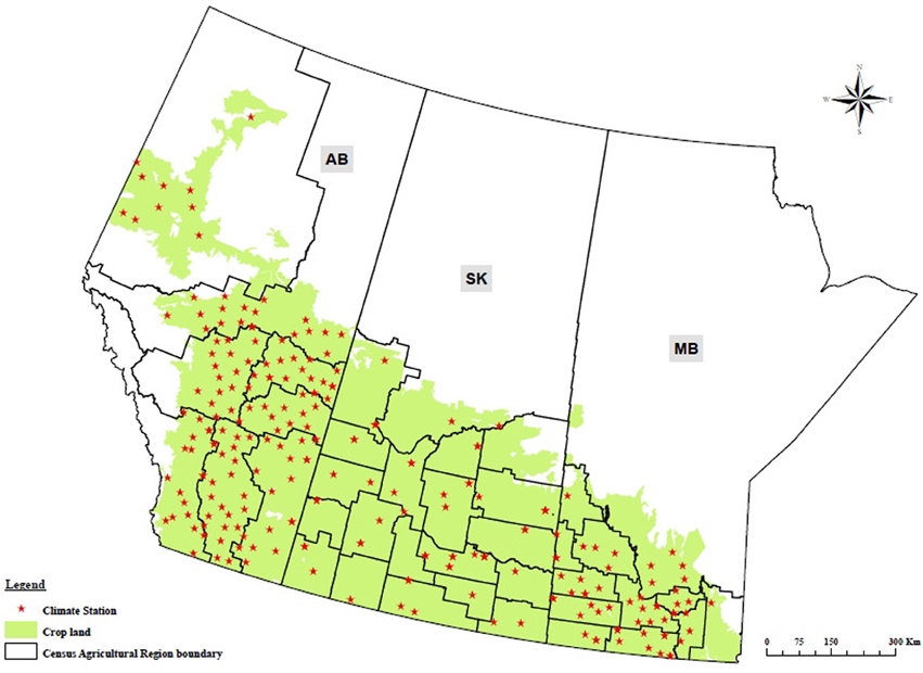
Figure 1. The major region of wheat production of the Canadian Prairies, encompassing the provinces of Alberta (AB), Saskatchewan (SK), and Manitoba (MB).

2.2. Data Sources

2.2.1. Agro-climate

Historical crop yield data from 1987 to 2011 for each of the CARs was obtained from the Field Crop Reporting Series of the Canadian Crop Condition Assessment Program (CCAP) of the Agriculture Division, Statistics Canada (Statistics Canada, 2007, 2012a,b). Station-based daily minimum/maximum temperatures and precipitation data were provided by Environment Canada and other partner institutions through the Drought Watch program, operated by the National Agro-climate Information Service (NAIS) of Agriculture and Agri-Food Canada (AAFC). This data was quality controlled and temporally-interpolated to provide a continuous, historical daily time-series from 1987 to 2012. A total of 259 climate stations were involved in the study (Figure 1). Agro-climatic variables considered in the model were growing-degree days (GDD) above an ambient air temperature of 5 °C, soil water availability (SWA), precipitation (P), and crop water deficit index (WDI) defined as WDI = (1 − AET/PET), where AET and PET are actual and potential evapotranspiration (Moran et al., 1994). AET and PET were computed using the Baier and Robertson algorithm (Baier and Robertson, 1996). Soil water availability (SWA) was defined, at any given time, as the percentage of available soil water holding capacity (AWHC). AWHC at the location of each climate station was determined from soil data obtained from the Soil Landscapes of Canada database from AAFC's Canadian System of Soil Classification (CANSIS, SLC Version 3.2, http://sis.agr.gc.ca/cansis/nsdb/slc/v3.2/intro.html). Crop-specific AWHC depends on soil type and is defined as the difference between soil water field capacity and wilting point, estimated as the cumulative amount of soil water to a maximum of 1 m soil depth or root-restricting soil layer under a difference in volumetric water at hydrostatic pressure of −33 and −500 kPa (Bootsma et al., 2005). Thermal-time (i.e., GDD-based) indices are widely referenced and used in crop development and growth response to temperature as well as crop heat stress and as an indicator of critical temperature thresholds for vernalization (e.g., 3°C of cold time) and for tracking crop developmental and growth. For example, in the case of cereal crops like barley and wheat indices are used to track the phenological stages of emergence, tillering, stem elongation, heading/flowering/anthesis, ripening, or for oilseeds like canola: sowing/germination, emergence, leaf initiation, stem elongation, bud formation, flowering, pod development, maturity (Ferris et al., 1998; Bootsma et al., 2005; Carew et al., 2009; Robertson et al., 2013). Nonetheless, other indices or measures of thermal-time requirements for crops such as biometeorological time (BMT) may be more accurate when crop end-use quality aspects are of interest, which for wheat includes: flour protein, farinograph dough development time and farinograph stability (Saiyed et al., 2009). Station-based minimum/maximum temperatures, precipitation and AWHC were input into a crop-specific soil water balance equation called the Versatile Soil Moisture Budget (VSMB) to generate the corresponding agro-climatic indices for each climate station at a daily time step (i.e., GDD, SWA, AET, PET) (DeJong, 1988; Baier and Robertson, 1996). More than one climate station was referenced within most CARs, but the number of stations within a given CAR did vary. In generating the agro-climate indices using VSMB, the start and end of growing season is determined by the accumulation of sufficient heat units and soil moisture. Daily agro-climatic values were temporally-averaged by month. We provide a summary of our data sources used in simulating, training and validating the forecasting model in Table 1.

TABLE 1

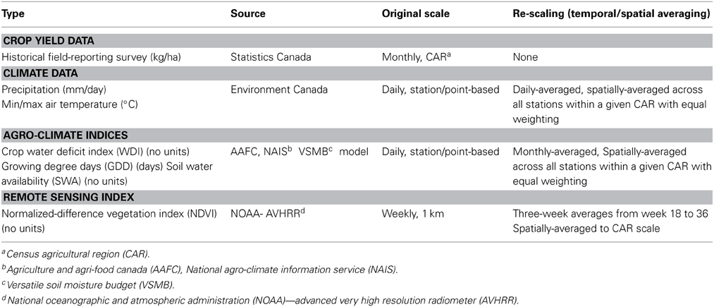
Table 1. Data integrated for simulating, training and validating the forecasting model across 1987–2012.

2.2.2. Satellite, remotely-sensed indices

ındent Normalized-difference vegetation index (NDVI) was also included as a predictor of yield. It is defined as NDVI= (ρNIR − ρRED)/(ρNIR + ρRED), where ρNIR and ρRED are the near-infrared and infrared portions of the electromagnetic spectrum of (0.75–1.5 μm or 841–876 nm) and (0.6–0.7 μm or 620–670 nm), respectively. This index is based on the contrast between the maximum absorption in the red due to chlorophyll pigments (0.4–0.7 μm) and the maximum reflection in the infrared by leaf cellular structure (0.7–1.1 μm) (Habourdane et al., 2004). The NDVI historical time-series were then combined to generate weekly composites south of 60° latitude (i.e., across the agricultural land area of Canada). The values of ρVIS and ρNIR are bounded between 0 and 1. NDVI itself varies between −1 (indicating no vegetation) and 1 (indicating dense vegetation). Weekly NDVI imagery data was compiled from historical data from the Advanced Very High Resolution Radiometer (AVHRR, 1 km resolution), U.S. National Oceanographic and Atmospheric Administration (NOAA) for years 1987–2012. Further quality control and processing in generating NDVI weekly composites was conducted (Reichert and Caissy, 2002). NDVI values were not crop-specific. Weekly NDVI indices from Julian week 18 to 36 (i.e., May to September) of each year were aggregated into 3-week moving means.

2.3. Forecasting Methodology

The integrated methodology includes possible crop-specific input data, and additional auxiliary indices that can be integrated and involved various modules and different computational steps (Figure 2). The forecast model was coded using the R Statistical Language (Version 2.15.3, R Development Core Team) (R Foundation, 2013) and made use of the following R library packages: MASS, robustbase, impute, WGCNA, np, mnormt, mcmc, tmvtnorm, Caret, and randomforest. The model's leading, tuning parameters and their library association, description and default values are summarized in Table 2.

FIGURE 2

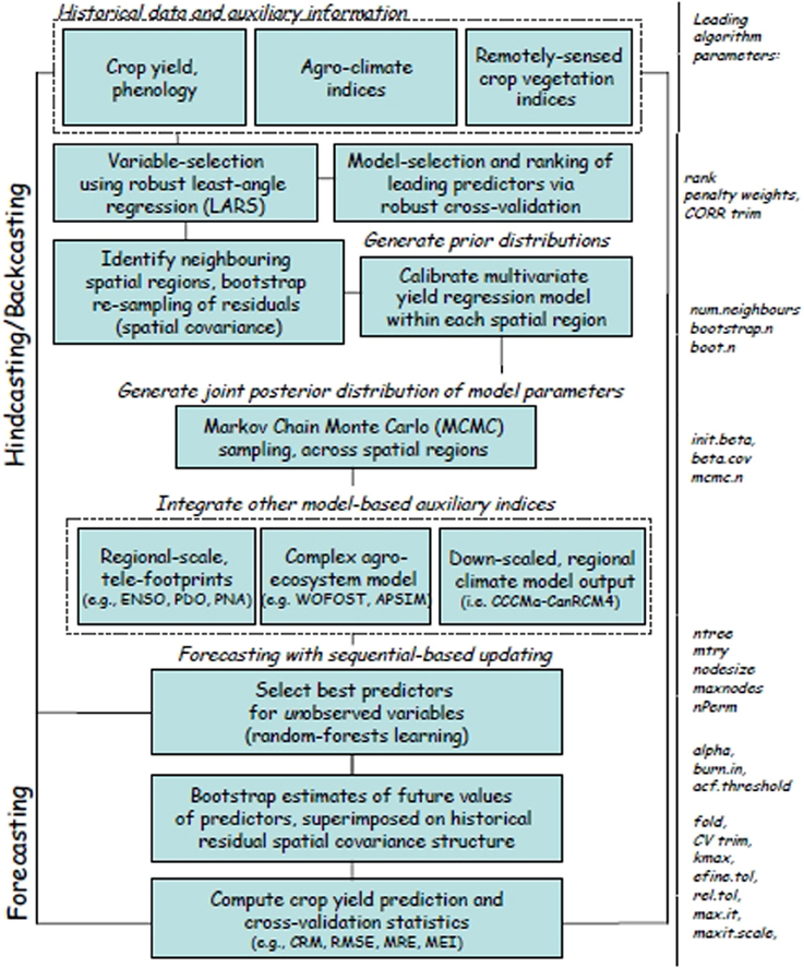
Figure 2. Major components of the sequential, spatial-based Bayesian forecasting model of regional-scale crop yield. Model parameters that are tuned and fixed within each model component are identified to the right. The procedure consists of calibration and a prediction steps. Hindcasting/ backcasting via leave-one-out cross-validation (LOOCV) is performed using the input data as training data. Sequential-based forecasting is accomplished via the random-forests learning algorithm. This methodology is able to integrate other possible auxiliary historical indices, such as regionally-downscaled indices derived from El-Nino Southern Oscillation (ENSO) index, Pacific Decadal (PDO), and the Pacific North American (PNA) climate teleconnection index. Forecast indices generated from complex agroecosystem models, such as WOFOST (WOrld FOod STudies, Wageningen UR) agricultural production model and APSIM, the Agricultural Production Systems sIMulator. Forecast indices derived from downscaled future CCCma-CanRCM4 denotes CanRCM4 regional climate model (RCM) scenario output produced by the Canadian Centre for Climate Modeling and Analysis (CCCma) for the North American region with a horizontal grid resolution of approx. 25 km and available at: http://www.cccma.ec.gc.ca/data/canrcm/CanRCM4/ could, in the future, also be integrated for generating regional yield forecasts. Adapted from Kouadio and Newlands (2014), with permission.

TABLE 2

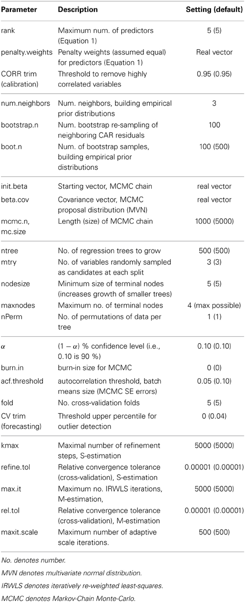
Table 2. Leading parameters (name, R library association, description, setting) of the integrated forecasting model.

2.3.1. Model calibration and training

The forecasting equations are based on Bayesian theory, and are an adaptation of a Bayesian auxiliary variable approach of Tanner and Wong (1987). These equations are used to jointly estimate and predict the underlying “environmental” state (i.e., prescribed by a set of agro-climate variables), the set of model parameters, including any additional auxiliary variables (e.g., remotely-sensed indices). Our statistical problem involves the prediction of future state and response, so is hereafter termed forecasting. Some ambiguity or discrepancy in terminology exists in the ecological and statistical sciences in regard to forecasting to better distinguish relevant terminology. Here, we adopt the terminology of Luo et al. (2011) in defining forecasting, prediction, projection, and prognosis, where forecasting involves a probabilistic statement on future states of an ecological system after data are assimilated into a model, prediction generates future states of an ecological system based on logical consequences of model structure, projection generates future states of an ecological system conditioned upon scenarios, and prognosis is a subjective judgment of future states of an ecological system. There are numerous methodological and practical advantages conferred by introducing auxiliary variables in an estimation and forecasting problem: (1) when computing the likelihood density of the observed data, f(y|θ) is analytically intractable, (2) when the inclusion of the auxiliary variables simplifies or improves the computation using Markov-Chain Monte-Carlo (hereafter, MCMC), whereby, f(y|x,θ) is a more complete data likelihood, and can be computed faster than the observed data likelihood, f(y|θ), (3) when a statistical problem involves latent or hidden variables, (4) when underlying states are controlled by dynamic processes occurring at multiple spatial and temporal scales (i.e., hierarchical problem), (5) when spatial interpolation and/or upscaling of point- or site-based data is impractical due to data sparsity and/or high spatial heterogeneity, and fine- and coarser-grained information must instead be integrated, (6) a response has a strong spatial dependence and estimation and forecasting is needed across a large spatial region, (7) when auxiliary variables track a response variable faster (i.e., near-real time), reducing delay, and (8) to improve a sequential forecast, by conditioning it at a given fixed or variable time-step.

2.3.2. Bayesian inference

Bayesian inference uses Bayes' rule to update the probability estimate for a hypothesis as additional evidence is learned, given by;

$\begin{array}{cc}p(H|E)\propto p(E|H)p(H),& (1)\end{array}$

where H is any hypothesis whose probability is influenced by data or observational evidence E, p(H) is the prior probability (probablity of H before E is observed), p(H|E) is the posterior probability of H after E is observed. p(E|H) is the probablity of observing E given H, also called the likelihood, where p(E) is the marginal likelihood or evidence. Bayes' rule therefore states that the “posterior probability is proportional to the prior times likelihood,” or similarly, “posterior is prior times likelihood over evidence.” The posterior is the result of updating our prior information with data (i.e., learning). Since the denominator does not depend on any H, it acts as a proportionality or normalization constant, and is obtained by averaging the “prior times likelihood” (i.e., numerator) over all possible hypotheses, H, such that,

$\begin{array}{cc}p(H|E)=\frac{p(E|H)p(H)}{p(E)};p(E)={\displaystyle {\int }_{H}p}(E|H)p(H)dH,& (2)\end{array}$

If we observe data, y, from a sampling density (i.e., distribution of the data), p(y|θ), where θ is a vector of parameters, and assign θ a prior p(θ), then, following from Equations (1, 2), the posterior density of θ is then;

$\begin{array}{cc}\begin{array}{l}p(\theta |y)=\frac{p(y|\theta )p(\theta )}{p(y)}\propto p(y|\theta )\hfill \\ p(\theta );p(y)={\displaystyle {\int }_{\theta }p}(y|\theta )p(\theta )d\theta .\hfill \end{array}& (3)\end{array}$

We introduce underlying state variables, q, (referred to as a Bayesian data augmentation, auxiliary or latent variable approach). The resultant joint posterior probability, taking into account both the θ parameters and the state variables, is given by;

$\begin{array}{cc}p(\theta ,q|y)\propto p(y|q,\theta )p(q|\theta )p(\theta )& (4)\end{array}$

The posterior of model parameters is then;

$\begin{array}{cc}p(\theta |y)={\displaystyle {\int }_{q}p}(\theta ,q|y)dq& (5)\end{array}$

Because the necessary integration to obtain the posterior distribution is analytically intractable, MCMC using the Metropolis-Hastings algorithm is typically used to obtain a sample from the joint posterior distribution of q and θ (Albert, 2009).

We assume that the parameters, θ, have a multivariate normal distribution (MVN) as the conjugate prior density. The Monte-Carlo standard errors and confidence intervals are computed using the method of batch-means (i.e., that generally requires posterior samples of at least 1000) (Jones et al., 2006).

For sequential-based forecasting, we adopt a state-space modeling framework, and express the probability densities above, as functions of a set of observed, p(y_t|x_t, θ), and underlying process, p(x_t|x_t−1, θ) discrete states of a dynamic system, for a sequence of times t = (1, …, T), that evolve from an initial state, p(x₁, θ).

If we denote and discretize any auxiliary explanatory variables, denoted as z_t, then, Equation (4), can be re-expressed (Tanner and Wong, 1987; King, 2012), as;

$\begin{array}{cc}p(\theta ,z|y,x)\propto p(y|x,\theta ,z)p(x|\theta ,z)p(z|\theta )p(\theta )& (6)\end{array}$

where,

$\begin{array}{cc}\begin{array}{l}p(y|x,\theta ,z)={\displaystyle \prod _{t=1}^{T}p}(y_t|x_t,\theta ,z_t); p(x|\theta ,z)={\displaystyle \prod _{t=1}^{T}p}(x_t|z_t);\\ p(z|\theta )=p(z_1){\displaystyle \prod _{t=2}^{T}p}(z_t|z_{t-1}).\hfill \end{array}& (7)\end{array}$

The x_t denote environmental states (i.e., a vector X of agro-climate variables or indices), and z_t denote states of additional auxiliary explanatory variables (i.e., a vector Z of remotely-sensed variables or indices). At each iteration of an MCMC algorithm, the model parameters and auxiliary variables are updated. One can further identify different spatial regions, s, such that x_t ← x_s,t and z_t ← z_s,t.

The posterior predictive or forecast density is either the replication of y given the model (denoted y^rep) or the prediction of a new and unobserved y, (denoted y^new), given the model. This is the likelihood of the replicated or predicted data, averaged over the posterior distribution p(θ|y), given by;

$\begin{array}{cc}\begin{array}{l}p\left(y^{rep}|y\right)={\displaystyle {\int }_{\theta }p}\left(y^{rep}|\theta \right)p(\theta |y)d\theta ; or\hfill \\ p\left(y^{new}|y\right)={\displaystyle {\int }_{\theta }p}\left(y^{new}|\theta \right)p(\theta |y)d\theta \end{array}& (8)\end{array}$

We assume a linear model that, in matrix notation, for a general response vector, Y, is given by;

$\begin{array}{cc}Y=D\beta +ϵ,& (9)\end{array}$

under the distributional assumptions,

$\begin{array}{cc}Y|\beta ,{\sigma }^2,D~N_n(\mu ,\Sigma )~N_n(D\beta ,{\sigma }^{2}I)& (10\end{array})$

where D is the design matrix, β is a vector of unknown model parameters, and ϵ is a vector of independently and identically-distributed normal random errors with mean zero and variance σ². Our design matrix, D, involves two sets of explanatory variables, such that D=(X|Z), having columns x₁, …, x_np augmented with columns z₁, …, z_nq. N_n denotes the MVN of dimension, n, with mean μ, variance-covariance matrix Σ and I the identity matrix.

Crop yield within each CAR region was modeled as a multivariate regression equation with spatially-varying coefficients (Banarjee et al., 2004),

$\begin{array}{cc}\begin{array}{l}E(Y|\beta ,X,Z)={\widehat{y}}_{i,j}=({\gamma }_{i,0}+{\gamma }_{i,1}\times j)+{\alpha }_i{y}_{i,j-1}+{\displaystyle \sum _{l=1}^{n_p}{\beta }_{i,j}^{(l)}}{x}_{i,j}^{(l)}\\ +{\displaystyle \sum _{l=n_{p+1}}^n{\beta }_{i,j}^{(l)}}{z}_{i,j}^{(l)}\hfill \end{array}& (11)\end{array}$

where ${\widehat{y}}_{i,j}$ denotes the estimated or expected value of y_i,j, the crop yield for year j (i.e., to distinguish calibration yearly time-step from the forecast monthly time-step, denoted by t), where j = (2, …, T), within a given CAR, i, where i = (1, …, C). x^(l)_i,j and z^(l)_i,j denote the l predictor variables for i at time j. The total number of predictor (i.e., n_p agro-climate and n_q auxiliary remotely-sensed) is n = n_p+n_q. The coefficients, β^(l)_i,j are spatially and temporally-varying. Uncertainty, ε_s,i is independent and normally distributed (random error) with mean zero and variance σ²_i. The regression coefficients, γ_i,0 (yield intercept), and γ_i,1 (technology trend coefficient) are used to de-trend the yield data and α is a lag-1 autoregressive term. The technology trend accounts for historical increases in yield from genetics, management practices to improve soil fertility, water conservation and minimize soil erosion and nutrient leaching. The technology trend in yield was assumed to be linear. The inter-annual autocorrelation in yield was assumed to vary across CARs.

For the ith region, the design matrix, for fixed i, is given by Di = (X1i, X2i, …, Xnpi|Znp+1i, Znp+2i, …, Zni), which is associated with the full/complete model parameter vector, Θi = (γ0, γ1, α, βi, σ2i). In matrix notation,

$\begin{array}{cc}{D}_i=\left(\begin{array}{cccc}{x}_{i,2}^{(1)}& x_{i,2}^{(2)}& \cdots & x_{i,2}^{(n_p)}\\ x_{i,3}^{(1)}& x_{i,3}^{(2)}& \cdots & x_{i,3}^{(n_p)}\\ ⋮& & & ⋮\\ x_{i,T}^{(1)}& x_{i,T}^{(2)}& \cdots & x_{i,T}^{(n_p)}\end{array}|\begin{array}{cccc}{z}_{i,2}^{(n_p+1)}& z_{i,2}^{(n_p+2)}& \cdots & z_{i,2}^{(n)}\\ z_{i,3}^{(n_p+1)}& z_{i,3}^{(n_p+2)}& \cdots & z_{i,3}^{(n)}\\ ⋮& ⋮& & ⋮\\ z_{i,T}^{(n_p+1)}& z_{i,T}^{(n_p+2)}& \cdots & z_{i,T}^{(n)}\end{array}\right)& (12)\end{array}$

2.3.3. Robust regression

Robust regression is a specialized technique used in the model to ensure it is less sensitive to outliers and may be applied to situations of unequal variance (Khan et al., 2007, 2010). This technique was applied to account for heteroscedasticity and outliers in the historical data during model training and calibration. Heteroscedasticity occurs when the variance of an explanatory or predictor variable is dependent on its value. Robust regression also provides a flexible and general technique for modeling based on residuals, because it is less influenced by the presence of outliers. Variable-selection is then employed for prediction in the case where there are no significant outliers. Robust regression is a compromise between excluding outliers entirely from the analysis and treating all the data points equally, as it is done in ordinary least squares (OLS) regression. The idea of robust regression is to weigh the observations differently based on how well-behaved the observations are. Several approaches to robust estimation have been proposed, including R-estimators and L-estimators. However, M-estimators are more widely used because of their generality, high breakdown point, and efficiency. M-estimators are a generalization of maximum likelihood estimators (MLEs). Standard MM-type regression estimates use a bi-square re-descending score function and returns a highly robust and efficient estimator (with 50% breakdown point and 95% asymptotic efficiency for normal errors). The tuning parameters of lmrob, the R package we used to implement robust regression, comprises an MM-type robust linear regression estimator that consists of an initial S-estimate, followed by an M-estimate via regression that enables one to specify a breakdown point and asymptotic efficiency consistent with normal distributional assumptions (Koller and Stahel, 2011).

2.3.4. Bootstrap least-angle regression

Bootstrap robust least angle regression (B-RLARS) was applied in selecting the leading m ≤ n_q potential predictors from z¹, z², …, z^n_q after adjusting for the effects of x¹, x² …, x^n_p. Let z^1,*, z^2,*, …, z^m,* denote the leading n_q ranked variables. A final, reduced model, with m* ≤ n_q predictors, is obtained with robust leave-one-out cross validation (LOOCV), by selecting auxiliary predictors from z^1,*, z^2,*, …, z^n_q,*, after adjusting for the influence of x¹, x² …, x^n_p (Khan et al., 2007, 2010).

Let the complete model design matrix, as D_C,T,(np+m*) following the selection of best-fit predictors. Let Ψ be the vector of model parameters corresponding to the joint distribution of D_C,T,(np+m*) (recall the model parameter vector is Θ_i = (γ₀, γ₁, α, β_i, σ²_i)). The conditional likelihood function of (y₂, y₃, …, y_n) given y₁ is then;

$\begin{array}{cc}\begin{array}{l}f\left(y_2,\dots ,y_n|y_1,\Theta ,D_{C,T,(n_p+m^{\ast })}\right)\\ =f\left(y_2|y_1\right)f\left(y_3|y_1,y_2\right)\cdots f\left(y_n|y_1,y_2,\dots ,y_{n-1}\right)\\ =N\left({\gamma }_0+2{\gamma }_1+{\displaystyle \sum _{l=1}^{n_p}{\beta }_2^{(l)}}{x}_2^{(l)}+{\displaystyle \sum _{l=n_{p+1}}^n{\beta }_2^{(l)}}{z}_2^{(l)}+\alpha y_1,{\sigma }^2\right)\\ \times N\left({\gamma }_0+3{\gamma }_1+{\displaystyle \sum _{l=1}^{n_p}{\beta }_3^{(l)}}{x}_3^{(l)}+{\displaystyle \sum _{l=n_{p+1}}^n{\beta }_3^{(l)}}{z}_3^{(l)}+\alpha y_2,{\sigma }^2\right)\\ \times \cdots \times N({\gamma }_0+n{\gamma }_1+{\displaystyle \sum _{l=1}^{n_p}{\beta }_n^{(l)}}{x}_n^{(l)}\\ +{\displaystyle \sum _{l=n_{p+1}}^n{\beta }_n^{(l)}}{z}_n^{(l)}+\alpha y_{n-1},{\sigma }^2),\end{array}& (13)\end{array}$

where the CAR subscript, i, was omitted. Given that (y₂, …, y_n) is independent of Ψ given y₁, Θ, and D_{C,T,(np + m*)}, it follows that;

$\begin{array}{l}p\left(y_2,\dots ,y_n,D_{C,T,\left(n_p+m^{\ast }\right)}|y_1,\Theta ,\Psi \right)\\ =p\left(y_2,\dots ,y_n|y_1,\Theta ,D_{C,T,\left(n_p+m^{*}\right)}\right)\\ p\left(D_{C,T,\left(n_p+m^{*}\right)}|\Psi \right).\hfill \end{array}$

Under a fully Bayesian approach, prior distributions for both Θ and Ψ must be specified. We assumed a separation of variables, such that, p (Θ, Ψ) = p (Θ) p (Ψ), and constructed an empirical prior distribution for Θ by residual bootstrapping the data from neighboring CARs. Information from neighboring CARs was also considered, employing an approach previously outlined and cross-validated by Bornn and Zidek (2012). This boostrapping procedure was as follows: the neighboring CARs of each given CAR were identified and the calibrated yield regression equation was fit to the given CAR and other surrounding, neighboring CARs simultaneously. The fitted models from the set of CAR neighbors were then cross-validated using the data for the given CAR. The top k ranked CARs, which could comprise a single or multiple neighbors to a given CAR, were then finally selected based on obtaining the minimal cross-validation error. This method was found to generate a more meaningful prior distribution of the model parameters by providing additional spatial covariance support (i.e., considers the residual spatial covariance between CARs). The joint posterior density function can be expressed as;

$\begin{array}{cc}p(y^{new}|y)={\displaystyle {\int }_{\theta }p}\text{}\left(y^{new}|\beta ,{\sigma }^2\right)p\text{}\left(\beta ,{\sigma }^2|y\right)d\beta d{\sigma }^2& (14)\end{array}$

The model predicted future values of the model variables (i.e., forecasted) within a given CAR using only the information from selected model predictors. This assumed a Gaussian prior distribution for each predictor variable, as a conjugate prior for the joint multivariate Gaussian posterior likelihood distribution. It is well-known that choosing a conjugate prior ensures that the resulting posterior distribution is of the same distribution family as the prior (with a closed-form solution), and helps to avoid over-fitting on small training samples. However, the selected predictor variables were determined not to be good predictors of one another and were uncorrelated (results not shown here). For this reason, the forecast method instead uses the entire set of available variables when selecting the best subset of predictors that jointly estimates the unobserved values of future variables. This was first accomplished for each CAR using the multi-variate adaptive regression splines (MARS) non-parametric algorithm, but was later substituted to use the Random Forests algorithm (Chipanshi et al., 2012; Newlands and Zamar, 2012; Kouadio and Newlands, 2014). The random forests algorithm proved to be more computationally efficient and accurate because it created multiple bootstrapped regression trees without pruning and averages the outputs, very effective in reducing variance and error in high dimensional data sets (Breiman, 2001; Chen et al., 2012). Also, by incorporating non-parametric Bayesian priors, we realized that our methodology would be more flexible and generally applicable in modeling with a wide set of variables and indices. It would also not have to assume a conjugate prior, which in many realistic or real-world cases is inappropriate. Model complexity is automatically determined by the model selection method we used because it specifies a maximum number of predictors (R-LARS followed by robust cross-validation).

2.4. Sensitivity Analysis and Validation Methodology

Dynamic sensitivity analysis was conducted by simulating the model for different input settings of the leading parameters. We also experimented by including and withholding precipitation (P) as an input variable (i.e., a variable with high stochasticity) to evaluate the change this had on forecast error. Ranges for these simulations were set by considering both default values provided in statistical literature linked with the R library code and values prescribed from the application of various algorithms to real-world data, as in the case of the random forest algorithm parameters.

The goal of cross-validation was to estimate the expected level of fit of a model to a data set that was independent of the data that were used to train the model. We cross-validated our model forecasts against historical data (1987–2011) by backcasting/hindcasting involving statistical bootstrapping and then leave-one-out cross-validation (LOOCV). The LOOCV selects a single (i.e., year) observation from the original full record as a sample of validation data, and the remaining observations as the training data. This was repeated such that every observation that exists in the sample (i.e., year) was used once as validation data. We performed an additional test of this cross-validation procedure by removing more than just 1 year of data at a time. This considered samples (K) of 1–5 years, following a K-fold cross-validation procedure. This additional test evaluated how robust the forecasts were to removal of training data/loss of input information termed forecast degeneracy. The model was also forecasted for the 2012 growing season and its output was compared to available statistical survey data across a range of spatial scales. In 2012, a total of 64% of land across the Great Plains/Midwestern United States is under abnormally dry to exceptional drought conditions (United States Department of Agriculture (USDA) Drought Monitor). NOAA has reported that the January–June period in 2012 was the warmest first half of any year on record for the contiguous United States, and the warmest the area has ever experienced since the dawn of record-keeping in 1895 (United States National Climatic Data Center, NCDC). In 2012, nearly 50% of corn and 37% of the soybeans grown in the United States were rated poor to very poor, with three-quarters of US cattle acreage in drought-affected areas. As this year exhibited such extreme conditions, it provided data with high environmental variability and a strong test of the accuracy and robustness of the model's forecasting methodology.

3. Results

3.1. Observed Variability

The observed variability of the agroclimate and remotely-sensed vegetation variables was considerable when pooled across CARs and years within the study region (Figure 3). In these box-plots (and throughout this paper), the solid line indicates the median error, with ends of the box indicating the upper and lower quartiles as a measure of data spread spanning 50% of the dataset and eliminating the influence of outliers. The whiskers are the two lines outside of the box that extend to the highest and lowest data values. An increasing trend in growing season mean-monthly precipitation (mm) (see inset a) was evident, explained by frequent and larger convective-driven storm events deliver rainfall across the region, accompanying increased summer temperature. Over-winter precipitation and accompanying spring thaw in May raised crop available water and reduces the soil capacity to store available water (inset b) until later in the season, when rainfall decreases (inset a) and significant soil water evaporative losses typically occur. This pattern of variability was consistent with the observed increase of crop water deficit index (WDI) (inset c). Lower/upper quartiles for GDD ranged between 180 and 450 GDD over the growing season, with 180 on average accumulated by end of May. Over the years in the climate station record, many of the CARs experienced extreme rainfall (as outliers in the box-plot of distribution quartiles). CARs also experience extreme temperatures in the middle of the growing season, signified by numerous outlier values in June from the plot of the GDD index (degree days above 5°C) (inset d). The variability of AVHRR-based NDVI (Figure 3, inset E) identified many outlier CARs that are situated far outside of the main distribution quartiles, indicating a general tendency for over-estimation of NDVI early in the growing season, and under-estimation mid-season, likely due to surface water backscatter.

FIGURE 3

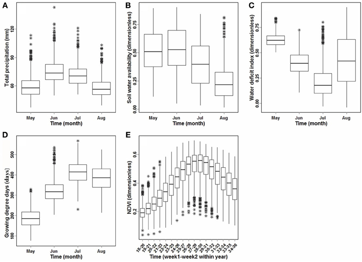
Figure 3. Observed distribution and variability of agro-climate and NDVI variables, through the growing season (May–September) based on historical data, 1987–2011. (A) Average total monthly precipitation (mm/month), (B) average soil water availability (SWA) (as % AWHC) (no units), (C) average crop water deficit index (WDI) (no units), (D) sum of growing degree days (GDD) (degree-days), and, (E) 3-week averaged AVHRR NDVI (no units).

3.2. Model Sensitivity

The sensitivity of forecasts was tested by simulating the model under changes in the: (1) number of predictors, (2) threshold for removing correlation variables (CORR trim), (3) threshold for the upper percentile for identifying outliers in cross-validation (CV trim), and (4) chain-size specified in the MCMC-simulation sampling from the joint posterior distribution (Equation 14) (Figure 4). These results tracks the change in CAR-based root-mean-square error (RMSE) uncertainty in forecasted yield versus each of the leading design parameters, whereby CORRtrim must be greater than 0.93 and a CV trim must be a value between 0.01 and 0.04 to minimize RMSE. These parameters were regionally-calibrated or tuned and set to 0.95 and 0.04, respectively. MCMC chain-size did not have a large effect on the median, or 10% and 90% percentiles or forecast RMSE uncertainty. The sensitivity to MCMC chain-size did not appear to change through the growing season, as the curve slopes were mostly flat for July, August and September. Therefore, we set the chain-size to a reasonable, mid-point value of 1000 to reduce run-time without any substantial loss of precision. A minimum of four predictors minimized RMSE. The inclusion of additional predictors, such as standard deviation of each of the predictor variables, did not make a significant difference (i.e., neither raised nor lowered forecast uncertainty). An additional sensitivity test of model on the effect of including precipitation (P) on forecast uncertainty was conducted (Figure 5). Selected regression results are summarized for two CARs that generated the best and worst regression fits (Figure 6). Scatterplots of observed versus predicted yield (A,B), residual versus predicted yield (C,D), and the relative importance or proportion of observed variance explained by each of the best-fit selected predictors (E,F) were generated. Model error reduces when considering from one to up to three predictors. Model accuracy increased when NDVI was included with the agroclimate variables (i.e., WDI, GDD, SWA) and year. Based on these findings, the default maximum number of model predictors was set to be five to regionally-calibrating yield across all the CARs in the study region. This sensitivity analysis identified whether all or a subset of these variables are necessary to obtain a best-fit in each CAR. For instance, with both agroclimate and NDVI indices as predictors, WDI, year and NDVI were selected in CAR 4741. When we constrained model input to NDVI only, RMSE for this region became very large, and is why CAR 4741 appears as an outlier for the “NDVI,” and is no longer an outlier in the “agroclimate and NDVI indices” cross-validation run (see Figure 5, right inset). This was also the case for CAR 4607 and 4609, where NDVI and year were the only predictors selected by the variable-selection algorithm of the forecast model. Further sensitivity-checks were made by re-running the forecast model and examining the change of RMSE of the output for different values of other design parameters listed in Table 2. In many instances, no appreciable effect was measured to support or justify changing the default settings obtained from the scientific literature, as was the case for the random forest tree algorithm. Although planting date did vary across our region (mostly by 15 days min to max), it was not selected as a leading covariate of yield and when forced into the model also did not have a significant effect on RMSE uncertainty, so we fixed this variable.

FIGURE 4

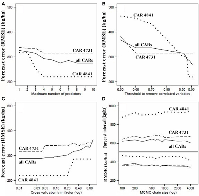
Figure 4. Sensitivity of forecasted error in yield (RMSE, kg/ha) (y-axes) to leading model design parameters (x-axes). The solid line, dotted, and dashed lines track the median yield across: all CARs, CAR 4841 (low sensitivity case), and CAR 4731 (high sensitivity case), respectively, for: (A) maximum number of predictors (trim factor to 0.04 and number of predictors varies from 1 to 10), (B) CORR trim factor (i.e., threshold for removing correlated variables), with the maximum number of predictors set to 5, (C) CV trim factor (i.e., a parameter of the lmrob() R library algorithm of the robustbase package that is a percentage for the upper percentile of observations to drop based on their cross-validated errors). The correlation trim factor was set to 0.04 on this sensitivity run, and number of predictors was set to 5 and the x-axis is in log scale, and (D) shows two panels divided by the solid horizontal line—the upper panel shows the range defined by the difference between the 10% and 90% percentiles of forecast yield in relation to changes in the MCMC chain size (mcmc.n). This considered all CARs and years of historical input data (i.e., 1987–2011). The three lines are the results for July (dotted), August (dashed), and September (solid). The lower panel tracks RMSE in forecasted yield corresponding to the same monthly forecasts in the upper panel.

FIGURE 5

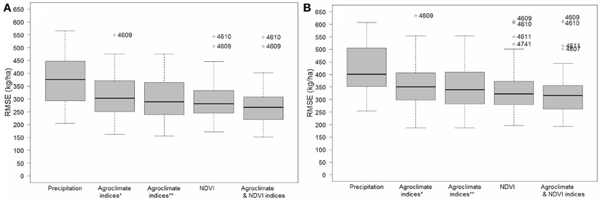
Figure 5. Sensitivity of forecast error (i.e., Root-mean-squared error variance, RMSE) for different combinations of selected agroclimate variables and NDVI. (A) Forecasted yield in 2012, and (B) cross-validated (LOOCV) (i.e., backcasted) forecast yield. The predictors sets considered in each run were: Precipitation (P); agroclimate variables of crop water deficit index (WDI), growing degree-days (GDD), soil water availability (SWA), where * denotes P is not included, and ** denotes P is included; NDVI; WDI, GDD, SWA, and NDVI. Note: seeding date was assumed fixed, and year, t, was included as an additional input variable in all the sensitivity runs. The ID's of outlier CARs are indicated.

FIGURE 6

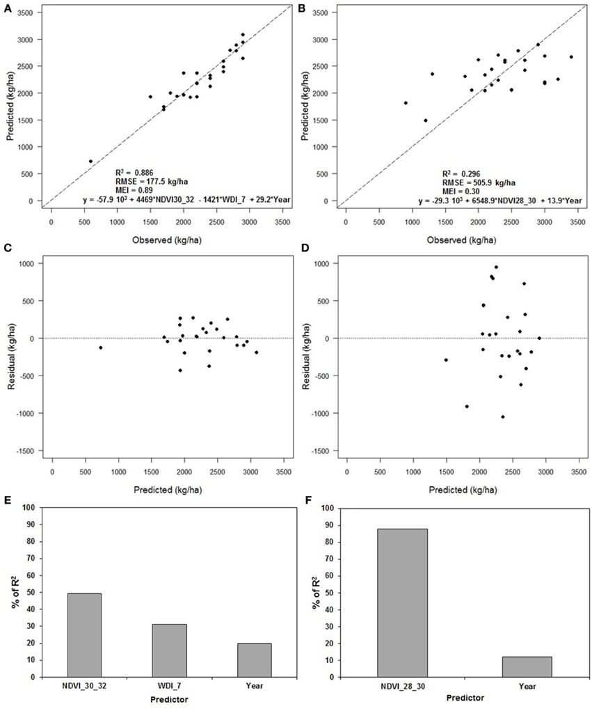
Figure 6. Selected diagnostic results from the multivariate regression of crop yield for the best overall fit (CAR ID 4840, left panels) and worst overall fit (CAR ID 4609, right panels). Scatterplots of observed versus predicted yield (A,B), residual versus predicted yield (C,D) and the relative importance or proportion of observed variance explained by each of the best-fit selected predictors (E,F) are provided. NDVI-30-32(28-30) denotes the 3-week moving average NDVI for Julian weeks 30–32, and WDI-7 denotes monthly-average of water deficit index in July.

3.3. Model Validation

The spatial pattern of model forecast uncertainty (RMSE) across all the CARs was generated for different combinations of the input predictors (Figure 7). Change in RMSE for many of the CARs was dependent on how the model was constrained in selecting only the prescribed maximum number and type of predictor variable. Combining both NDVI and agroclimate predictors enabled minimal uncertainty in most CARs (i.e., within 150–250 kg/ha). However, there were CARs in northern Alberta (4860), central Saskatchewan (4730), and south-eastern Manitoba (4609 and 4610) for which uncertainty could not be appreciably reduced further.

FIGURE 7

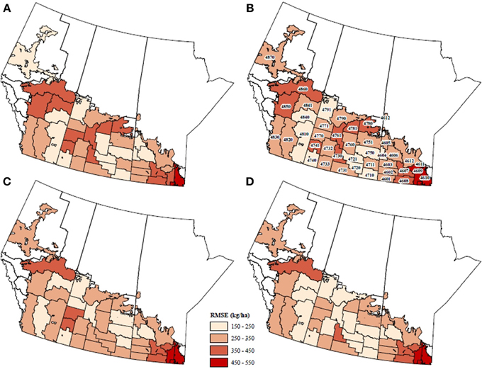
Figure 7. Spatial maps of forecast error (RMSE) for different combinations of predictors. The predictors sets considered in each run were: (A) WDI, GDD, SWA, P, (B) WDI, GDD, and SWA (i.e., no P), (C) NDVI, and, (D) WDI, GDD, SWA, NDVI. Note: seeding date was assumed fixed, and year, t, was included as an additional input variable in all the sensitivity runs.

Mean percent departures between historically observed and 2012 forecasted yield varied between under-estimation of 1–4% at the mid-point (i.e., July) of the May-October crop growing season, to over-estimation of less than 1% at end of season (i.e., September) (Table 3). This compares to a slightly higher mean percent departure based on independent, field crop-reporting yield data in 2012, of under-estimation of 3.6% mid-season, to less than 1% of over-estimation end-season (Table 4). Yield was forecasted for 2012 to be 3386, 2471, 2559 kg/ha in Alberta, Saskatchewan and Manitoba, respectively. Across the Canadian Prairies, forecasted yield was 2803 kg/ha, varying between 2513 and 3092 at the 90% confidence level (Figure 8). Further inspection of yield variability within the two CARs with the highest forecast error (i.e., CV > 18%) for CARs (4610 and 4860) revealed that they exhibit unique patterns that departed from our model assumptions and variability observed within other CARs (Figure 9). Sample autocorrelation functions (ACFs) of historical crop yield that track the strength of the inter-annual dependence in yield between successive years, revealed an extended (i.e., 3-year duration) correlation with a decaying or tapering pattern for CAR 4610, indicating an autoregressive random process of order 3, AR(3), with a positive coefficient. For CAR 4860, an alternating and tampering pattern was identified, indicating an autoregressive process of order 1, AR(1), with a negative slope coefficient.

TABLE 3

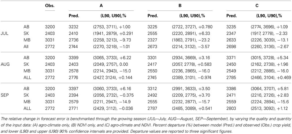
Table 3. Forecasting of 2012 spring wheat crop yield (kg/ha) across the Canadian Prairie provinces (AB—Alberta, SK—Saskatoon, MB—Manitoba, All—Prairies).

TABLE 4

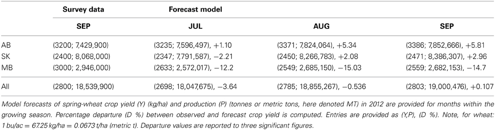
Table 4. Comparison of model forecasts (using both agro-climate and NDVI indices) to Statistics Canada field crop-reporting survey data (CCAP), upscaled to the provincial scale.

FIGURE 8

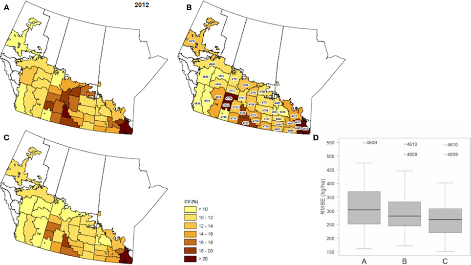
Figure 8. Left: Crop yield forecast for 2012—spatial distribution of model error (CV %) for all CARs in the study region in forecasting spring wheat crop yield in 2012, with: (A) agroclimate indices (WDI, GDD, SWA), (B) NDVI, (C) WDI, GDD, SWA, P, NDVI. Right: (D) Forecasted error in 2012, pooled across all CARs for the different input cases (A–C).

FIGURE 9

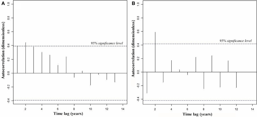
Figure 9. Identified patterns of autocorrelation functions (ACFs) of historical crop yield for CARs with high RMSE forecast error. (A) CAR 4860 with AR(3) process with positive slope, and (B) CAR 4610 with AR(1) process with negative slope.

The RMSE uncertainty associated with the median forecast within CARs was 330 kg/ha, varying between 280 and 360 kg/ha at the 25% and 75% percentile, respectively, from LOOCV analysis of forecasts across all historical years. For the 2012 growing season, the median was less at 270 kg/ha, ranging between 230 and 300 kg/ha. When cross-validating the model forecasts, the number of years that were left out was varied from 1 to up to 5 years at a time (Figure 10). While we utilized a LOOCV procedure with 1 year left out at a time. The additional cross-validation results from the K-fold cross-validation led support for this specification, indicating that specifying any higher number of years left out at a time, only reduced the model's forecast accuracy (RMSE error) by less than 5%.

FIGURE 10

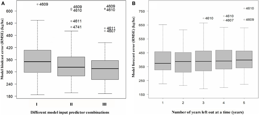
Figure 10. (A) Variation in model hindcast/backcast error from leave-one-out cross-validation (LOOCV) (RMSE in kg/ha) for three different combinations of input predictors: (I) Agro-climate indices (WDI, GDD, SWA), (II) Remote-sensing index (NDVI), and (III) Agroclimate and NDVI index (WDI, GDD, SWA, NDVI). A year effect is included in all cases. For case (III), the CAR 4610 is an outlier (as per the 2012 model forecast output results shown in Figure 5). Unlike the single year model forecast results for 2012, the LOOCV procedure that considers all possible combinations of missing data (i.e., years) in the historical input data, also identifies CAR 4609 as an outlier. (B) Variation in model forecast error (i.e., skill) in terms of “degeneracy” in the input data, simulated by increasing the number of years at a time that were left out in the LOOCV cross-validation procedure. Results correspond to a total of 1000 MCMC runs. CAR 4606 was excluded as it had only 7 years of missing data.

4. Discussion

4.1. Model Performance

Model forecasts were sensitive to both the choice of design parameters and the set of input explanatory (predictor) variables. Agroclimate variables contributed significantly to improving overall multivariate regression fits across most CARs. The CARs, where the model performed the worst, only had NDVI and year as explanatory variables. However, NDVI did explain a significant portion of the observed yield variance in time and space (Figure 6). Because the sensitivity of forecasts to changes in the leading model design parameters was successfully minimized. This suggests that selecting the best predictors of yield within each CAR region, thresholding the detection of cross-correlation between predictors (so as to avoid multi-collinearity), combining information between neighboring CAR regions, and using robust regression to detect outliers, significantly improved robustness of the model's forecasts across the Canadian Prairies (i.e., a large study region).

A simple linear regression model to predict Canadian spring wheat crop yield and applied at the provincial scale achieved 53–77% accuracy relying solely on agro-climate indices (i.e., growing degree day (GDD), precipitation (P), actual/potential evapotranspiration (AET, PET) and crop water deficit index WDI) (Qian et al., 2009). At the provincial scale, percent departure values for 2012, and LOOCV results across the entire region (all CARs) supports that our integrated model forecasts attains a higher overall or forecast skill (CV < 10% or accuracy > 90%), even accuracy does vary between CARs. With further adjustment to our model to allow for alternating autocorrelation with negative slope coefficients, we infer the two CARs with the highest uncertainty would also be greatly improved. Seeded area, irrigation and/or pests could also explain why these two CARs depart from all others, warranting further investigation. Also, without using agroclimate data, and using only satellite remote-sensing data (i.e., NDVI) was shown to predict hstorical wheat yield ranging between 47 and 80% accuracy at the CAR scale and across the Canadian Prairies (Mkhabela et al., 2011). Our findings show that while NDVI is a strong predictor of yield, combining agroclimate and NDVI indices substantially increases the accuracy and confidence in regional forecasts. One can also better discriminate between key ecological variables (i.e., temperature and available soil water) driving yield variability in time and space, which would otherwise, not be possible when only considering a single index.

Globally, wheat accounts for 20% of calories consumed. It is one of the most important crops, alongside rice and maize (corn). Our integrated model forecasted spring wheat yield for 2012 of 2803 kg/ha (Canadian Prairies) and associated uncertainty of 2513–3092 at the 90% confidence level agrees to close to 0.1% of end-of-season field survey yield, and 4% at the start of the growing season. This forecasted yield for 2012 compares reasonably well to independent crop insurance data for 1965–2007 on spring wheat yield across the Prairies accounting for a progressive increase of 0.8–1%/year technology-trend in yield during the period of 2007–2012. Crop insurance data indicated highest and lowest average yields of 4589 and 80.9 kg/ha in 2005 and 1988, respectively, and an overall historical average of 1991.2 kg/ha (Robertson et al., 2013). Total factor productivity (TFP) growth rate in crop production (1980–2004) for the Canadian Prairies was estimated to be 1.77%, where technology change contributes close to 83%, in addition to the smaller contributions from scale effects and changes in the degree of technical efficiency (e.g., improved machinery or crop genetics). TFP has, historically, increased the most in Manitoba, explained in part by reduced use of summer fallow, but historically has lagged within Alberta (Stewart et al., 2009). Also, Canadian Plant Breeder Rights (PBR) qualifying wheat cultivars and improved soil quality have increased wheat yield by 37.2 (1%) to 54.5 kg/ha (2%) within the Canadian Prairies (Carew et al., 2009). Our forecast model could also better account for technology-change, rather than assuming a fixed, linear rate of productivity growth within each CAR based on historical data and trends. Instead, a more detailed equation involving percent of wheat seeded area, spatial cultivar diversity index, average cultivar age and annual cropland planted could be introduced (Carew et al., 2009) in addition to the year time trend already considered (that captures advances in non-genetic technology). However, this could make our regional-scale model too complex. The model generated robust forecasts of spring wheat yield for this extreme year 2012 based on historical data. It was also able to pinpoint two CARs in southern Manitoba that experienced extreme growing conditions in 2012, but also identify that yield within this area exhibits extended correlation with a duration of up to 3 years—very likely attributed to the impact of “persistent” drought and flooding conditions. While TFP has increased most in Manitoba, monthly rainfall variability is high within these two CARs, varying between 17 and 20%. More climate stations and rainfall data for these two CARs might therefore help to reduce forecast error in this region.

4.2. Model Limitations

Our model currently does not consider crop genetics and does not input cultivar-specific data on yield or their developmental and growth requirements, and does not select agroclimate or remotely-sensed predictors according to such cultivar-specific requirements. So, there is a further need to better understand how cultivar differences and genetics × management × environment interactions (i.e., G × M × E) could be used to temporally segment or partition input remote-sensing data for early, mid and late-season (or quick, medium and slow maturing) varieties. Mapping crop suitability spatially for different crop varieties could also enable a determination of the best spatial resolution to integrate agroclimate, remote-sensing vegetation and phenology indices in generating regional-scale forecasts.

Recent advances in multivariate time series segmentation methods, such as that described in Graves and Pedrycz (2009) could then be applied to historical remote sensing data to help automate the identification of transition points between stages directly from spatially-referenced, longitudinal time-series of yield obtained from culitvar crop-breeding field trials. We aim to further explore how the performance of our forecast model could be improved by considering crop genetics by including an auxiliary index based on APSIM agroecosystem model forecasts across a series of site-specific long-term cropping sites across the Canadian Prairies. The use of auxiliary indices derived from more complex models of agroecosystem soil, water, air and agronomic management interactions could offer further potential reductions in forecast uncertainty, and an ability to extend our seasonal forecasts and link them to longer-term yield forecasts.

Given that our model does not yet integrate crop phenology, cultivar differences, pest infestations, the interpretation and broader application of our current model to other regions and crops is limited. However, representing such differences at a regional-scale is still a big challenge due to lack of such data across large regions, so applying our model to other areas could generate useful insights for decision-makers, where a lack of data exists. Building a component to spatial track pest infestations from pest monitoring data, like that of wheat midge (Sitodiplosis mosellana), a common agricultural pest within most areas of the world where non-resistant wheat varieties are still grown, could also improve the reliability of the forecast model. With further improvement and extension of input data, and refinement of its design, we anticipate our forecast model could provide reliable and robust regional-scale crop yield forecasts. Alongside using our model to forecast crop yield, participatory workshops and stakeholder knowledge-sharing and engagement is critical for enabling open discussion of any real and perceived differences in model and farmer forecast skill. Such approaches have proved invaluable for improving forecast models and their relevance, impact and broader applicability (Pease et al., 1993; Potgieter et al., 2003; Roncoli, 2006; Crane et al., 2010).

4.3. Improving Forecast Skill

Several key improvements for our forecasting methodology and use of statistical algorithms for variable- and model- selection could be further explored. A more general autocorrelation function, which can account for extended patterns, could be tested. Also, heavier penalties for selecting predictor variables whose values are available late in the growing season could also be tested. This would make the selection of the best set of predictors through the growing season to be less constrained and dependent on historical patterns and thus more responsive to future environmental changes affecting yield. Also, tuning of the random forest algorithm parameters could be explored using the tuneRF R library set of algorithms. Even though future changes may be uncertain and depart significantly from historical trends, the necessity of an adequate length and quality of historical data does impose a requirement to partially- or fully-calibrated model-based forecasts using our integrated methodology. Recently, the accuracy in forecasting crop yield (i.e., wheat, barley and canola) also using NDVI remote-sensing and agroclimate data and employing multivariate linear regression and a variety of machine learning techniques other than the random forest tree algorithm, such as model-based recursive partitioning (MOB) and Bayesian neural networks (BNN) has been investigated (Johnson, 2013). Hierarchical clustering across the CAR regions was used for variable-selection. Based on a Mean Absolute Error (MAE)-based forecast skill score, reportedly multiple linear regression (MLR) achieves the highest skill for spring wheat and canola, while BNN and MOB are able to further increasing skill for barley. This may indicate that if new auxiliary agroclimate or remote-sensing indices are utilized which are non-linearly related or introduce a non-normal (e.g., highly skewed or multi-modal) probability prior distribution, or regional-scale climate and yields become more non-linearly related in the future, forecasting algorithms that are able to better deal with non-linearity may need to be substituted to ensure quality in crop forecasts. Here, substituting our MCMC algorithm with an integrated nested Laplace approximation (INLA) that could offer a computationally cheaper alternative. The INLA algorithm would enable representing agro-climate, remote-sensing or other predictors as functions that can be each fit to a different model with a different form of spatial dependence and degrees of non-linearity.

There are also several key improvements to the input data that could be undertaken. Assimilating additional climate station data within certain CARs that exhibit strong spatial heterogeneity (compared to other CARs) in temperature and precipitation could provide further reductions in forecast uncertainty. This could help reduce uncertainty, in addition to accounting for autocorrelation in these variables, within the two CAR's in southern Manitoba that showed highest RMSE that we speculate is due to localized drought and flooding conditions that have occurred there. Validating the agroclimate index for soil water availability (SWA) that was derived from the VSMB soil water model against other independent data would be informative before testing other available remotely-sensed indices (i.e., other than NDVI), such as EVI2 (Enhanced Vegetation Index) for this region could improve forecasting there. Integration of EVI2 remote-sensing index would incorporate the blue portion of the light spectrum and help to better track crop yield by reducing sensitivity of the NDVI to this backscatter. Also, summer storms can deliver large amounts of rainfall in the Canadian Prairies and even in semi-arid environments, sufficient long periods of sustained high rainfall can raise the water table (upper level of saturated soil-water zone) causing groundwater flooding and prolonged conditions of excess surface water, ponding and runoff. Integrating other remotely-sensed indices could be used to track waterlogging (excess water) between the development stages of tillering and anthesis. This would increase the reliability of the forecast model to recognize, respond and forecast yield under extreme conditions of increase rainfall intensity expected to occur in the future due to increased climate variability. Currently, precipitation was removed as a direct, leading predictor given it did not improve forecast accuracy because of its high variance. Instead, precipitation was indirectly factored into the WSI index. Nonetheless, precipitation, early in the growing season, can have a leading influence on attainable yield (He et al., 2013). For example, Bolton and Friedl (2013) have recently reported that significant precision in predicting corn yield in the United States can be achieved using the Normalized Difference Water Index (NDWI) (R² = 0.69 in semi-arid areas) as well as the two-band EVI2 of NASA's MODerate-resolution Imaging Spectroradiometer (MODIS) onboard NOAA's Terra satellite, predicting corn and soybean yield better than NDVI. From 2000 onwards, NDVI data, available the MODIS could also be utilized (MODIS, 250 m resolution, Level-2 Gridded (L-2G) surface reflectance data (collection V005)) (NASA, 2012). A statistical regression-based comparison of MODIS with AVHRR 16-day (i.e., bi-weekly) NDVI composite data indicates that for the row crop and small grains land cover classes, over 90% of the variation observed in MODIS NDVI is associated with variation in AVHRR NDVI values (Gallo et al., 2004). Findings from this comparison also indicate that there remains some residual cloud contamination in both data sets that contributes to outliers. Therefore, replacing AVHRR NDVI with MODIS NDVI post-2000 may not reduce the occurrence of outliers, unless cloud contamination is dealt with first. For this reason, AVHRR was deemed adequate for the purposes of our modeling, pending further quality control (i.e., explanation and subsequent reduction) of NDVI residual variance. Cloud removal, cropland area and boundary masking and other quality control measures for MODIS NDVI are described in Davidson et al. (2009). Leaf area index (LAI), soil-adjusted vegetation index (SAVI) could also be integrated and help track yield across different developmental stages based on existing evidence they correlate well with the different crop phenological stages (Kumar et al., 1999; Graves and Pedrycz, 2009). Other combined and improved spectral indices have been developed, validated to better incorporate non-linearity between NDVI and crop biophysical parameters and under water-limited conditions (Habourdane et al., 2004; Eitel et al., 2008; Smith et al., 2008). Further work could also optimize the model to the time period within the growing season that is the most sensitive and most significant for establishing final yield. So, instead of referencing WSI across the entire season, WSI for the most sensitive time period of crop growth could be used. It is important to highlight that inclusion of remote-sensing indices is not to complete replace field crop survey data in training and validating seasonal crop forecasts, but to supplement, improve and add value to such forecasts in both a spatial and temporal context.

5. Concluding Remarks

Our forecast modeling findings demonstrate that forecast skill at the regional-scale can be improved with an integrated approach involving the integration of different auxiliary indices (e.g., agroclimate and remotely-sensed) within a probabilistic, Bayesian framework that incorporates both data and model structural uncertainty. The need for improved operational forecasting methods is particularly urgent because forecasting models are so crucial for guiding and informing agricultural crop production, management and policy decisions. Models also provide forecasts with extended “early-warning” or lead-time, enabling stake-holders to better respond to potential impacts and emerging risks. Recent results from the world's largest standardized inter-comparison of ensemble-based model projections of climate change impacts on wheat crop yield calibrated against >300 field data-sets, reveals net-uncertainties of 20–30% CV when partially calibrated, and 2–7% CV for fully-calibrated models (Asseng et al., 2013). Such uncertainty is explained, in part, due to observed variability in climate, soil water holding capacity, sowing date and agronomic management (i.e., fertilizer application) (Asseng et al., 2013; Carter, 2013). Our findings indicate that by coupling satellite, remote-sensing with agroclimate data, forecast uncertainty in model-based crop yield forecasts can be further reduced to within the range of 1–4% (i.e., for spring wheat in the Canadian Prairies). This integrated methodology offers a consistent, generalizable approach for sequentially forecasting crop yield at the regional-scale. It provides a statistically robust, flexible way to concurrently adjust to data-rich and data-sparse situations, adaptively select different predictors of yield to changing levels of environmental uncertainty, and to update forecasts sequentially so as to incorporate new data as it becomes available. It also provides additional statistical information (i.e., bias, variance, sensitivity and cross-validation statistics) for better assessing the reliability of generated crop yield forecasts in time and space.

We aim to further apply our integrated forecast methodology to generate crop forecasts across Canada by embedding it within an operational forecasting system called the Integrated Canadian Crop Yield Forecaster (ICCYF). This operational decision-support tool with provide forecasts for all major Canadian crops with national coverage across all major agricultural areas. This will require the validation of our model for other major Canadian crops such as barley, canola and soybean. Operational crop outlooks likely will delivered by AAFC and publically-released in partnership with Statistic Canada's Crop Condition Assessment Program. With further extension and validation testing of this forecasting methodology to other major Canadian grain and oilseed crops (e.g., barley and canola), this method will provide a reliable approach for generating more rapid and lower cost crop forecasts each year, within the growing season, and across Canada's agricultural extent. Alongside our continued research work, further international collaborative efforts will seek to improve the design of a consistent and reliable international framework for crop yield and production forecasting and outlook reporting that integrates remote-sensing and agroclimate predictors (Nikolova et al., 2012). Our findings reported here demonstrate that our integrated methodology can provide robust and accurate regional-scale forecasts of spring wheat yield. It offers a flexible, scalable approach for integrating additional auxiliary indices, independent of spatial or temporal scale. In this way, it can integrate remotely-sensed vegetation or finer-scale indices based on field site data. Oursensitivity and cross-validation model findings also provide rigorous analytical testing of the relative benefits of using and combining difference and diverse sources of information in terms of better explaining and reducing uncertainty in model-based forecasts. This integrated method also provides additional statistical support for assessing the accuracy and reliability of model-based crop yield forecasts in time and space. We aim, in the future, to collaborate internationally in applying and validating the integrated forecasting methodology to other countries and continents that experience different regional climate and cropping conditions.

Conflict of Interest Statement

The authors declare that the research was conducted in the absence of any commercial or financial relationships that could be construed as a potential conflict of interest.

Acknowledgments

This research was funded under the Growing Forward One, Sustainable AGriculture Environmental Systems (SAGES) Program of Agriculture and Agri-Food Canada (AAFC), with additional support from AAFC's National Agro-climate Information Service (NAIS) and the Growing Forward Two, Canadian federal funding program. We thank Charles Serele (Federal Department of National Defence), Budong Qian and Richard Warren (AAFC) for their assistance in acquiring and manipulating agro-climate input data. We thank Andrew Davidson for help in processing and preparing the NDVI remote-sensing/earth observational data. We also acknowledge feedback from a broader set of government collaborators involved in the operational development and delivery of the crop outlook prototype tool: C. Champagne, P. Cherneski, B. Daneshfar, A. Davidson, X. Geng, E. Gorelov, D. Qi, R. Rieger, and D. Waldner from AAFC and F. Bedard and G. Reichert from Statistics Canada for their support and contributions. We thank R. Armstrong (AAFC) for analyzing the autocorrelation in the wheat data, and R. Carew, L. Townley-Smith, and B. MacGregor for feedback and discussions on this research linked with ecological and economic aspects. We also thank three anonymous reviewers for their feedback that helped to improve our manuscript. A prototype version of this forecast model for generating operational crop outlooks is called the Integrated Canadian Crop Yield Forecaster (ICCYF) has been coded and tested using the open source software and statistical libraries provided by the R Statistical Software (R Development Core Team, 2013). ArcGIS^TM, (ESRI^TM, Version 10, 2010) was used to visualize model output, processing spatial data and generating crop outlook maps. A user-guide is available with the R code for non-commercial and academic research. With further extension and testing of the forecasting method to other major crops and across Canada's agricultural extent, it is anticipated that a web-based portal will, in the future, deliver seasonal, operational crop outlook reports.

Supplementary Material

The Supplementary Material for this article can be found online at: http://www.frontiersin.org/journal/10.3389/fenvs.2014.00017/abstract

Footnotes

1. ^www.fao.org/giews/

References

Albert, J. (2009). Bayesian Computation with R. New York, NY: Springer Science-Business Media. doi: 10.1007/978-0-387-92298-0

CrossRef Full Text

Asseng, S., Ewert, F., Rosenweig, C., Jones, J., Hatfield, J., Ruane, A., et al. (2013). Uncertainty in simulating wheat yields under climate change. Nat. Clim. Change 3, 827–832. doi: 10.1038/nclimate1916

CrossRef Full Text

Asseng, S., Keating, B., Fillery, I., Gregory, P., Bowden, J., Turner, N., et al. (1998). Performance of the APSIM-wheat yield in Western Australia. Field Crops Res. 57, 163–179. doi: 10.1016/S0378-4290(97)00117-2

CrossRef Full Text

Baier, W., and Robertson, G. (1996). Soil moisture modelling - conception and evolution of the VSMB. Can. J. Soil Sci. 76, 251–261. doi: 10.4141/cjss96-032

CrossRef Full Text

Banarjee, S., Carlin, B., and Gelfand, A. (2004). Hierarchical Modeling and Analysis for Spatial Data. Monographs on statistics and applied probability, Vol. 101. New York, NY: CRC/Chapman and Hall (Taylor and Francis LCC).

Bastiaanssen, W., and Ali, S. (2003). A new crop yield forecasting model based on satellite measurements applied across the Indus Basin, Pakistan. Agric. Ecosyst. Environ. 94, 321–340. doi: 10.1016/S0167-8809(02)00034-8

CrossRef Full Text

Bolton, D., and Friedl, M. (2013). Forecasting crop yield using remotely sensed vegetation indices and crop phenology metrics. Agric. For. Meteorol. 173, 74–84. doi: 10.1016/j.agrformet.2013.01.007

CrossRef Full Text

Bootsma, A., Gameda, S., and McKenney, D. (2005). Potential impacts of climate change on corn, soybeans and barley yields in Atlantic Canada. Can. J. Soil Sci. 85, 345–357. doi: 10.4141/S04-019

CrossRef Full Text

Bornn, L., and Zidek, J. V. (2012). Efficient stabilization of crop yield prediction in the Canadian Prairies. Agric. For. Meteorol. 153, 223–232. doi: 10.1016/j.agrformet.2011.09.013

CrossRef Full Text

Breiman, L. (2001). Random forests. Mach. Learn. 45, 5–32. doi: 10.1023/A:1017934522171

CrossRef Full Text

Carew, R., Smith, E., and Grant, C. (2009). Factors influencing wheat yield and variability: evidence from Manitoba, Canada. J. Agric. Appl. Econ. 41, 625–639. Available online at: http://ageconsearch.umn.edu/bitstream/56649/2/jaae159.pdf

Carter, T. (2013). Multi-model yield projections. Nat. Clim. Change 3, 784–786. doi: 10.1038/nclimate1995

CrossRef Full Text

Challinor, A. (2009). Towards development of adaptation options using climate and crop yield forecasting at seasonal to multi-decadal timescales. Environ. Sci. Pol. 12, 453–465. doi: 10.1016/j.envsci.2008.09.008

CrossRef Full Text

Challinor, A., Slingo, J., Wheeler, T., Craufurd, P., and Grimes, D. F. (2003). Toward a combined seasonal weather and crop productivity forecasting system: determination of the working spatial scale. J. Appl. Meteorol. 42, 175–192. doi: 10.1175/1520-0450(2003)042<0175:TACSWA>2.0.CO;2

CrossRef Full Text

Chen, J., Li, M., and Wang, W. (2012). Statistical uncertainty estimation using random forests and its applications to drought forecast. Math. Probl. Eng. 2012, 1–12. doi: 10.1155/2012/786281

CrossRef Full Text

Chipanshi, A., Zhang, Y., Newlands, N. H., Hill, H., and Zamar, D. (2012). “Introducing the integrated canadian crop yield forecaster (ICCYF),” in Proceedings of the Workshop on the Application of Remote Sensing and GIS Technology on Crops Productivity Among APEC Economies, 1–14.

Crane, T., Roncoli, C., Paz, K., Breuer, N., Broad, K., Ingram, K., et al. (2010). Forecast skill and farmer's skill: seasonal climate forecasts and agricultural risk management in the southeastern united states. Weather Clim. Soc. 2, 44–59. doi: 10.1175/2009WCAS1006.1

CrossRef Full Text

Davidson, A., Howard, A., Sun, K., Pregitzer, M., Rollin, P., and Aly, Z. (2009). A National Crop Monitoring System Prototype (NCMS-P) Using MODIS Data: Near-Real-Time Agricultural Assessment from Space. Technical report, Agriculture and Agri-Food Canada (AAFC).

DeJong, R. (1988). Comparison of two soil-water models under semi-arid growing conditions. Can. J. Soil Sci. 68, 17–27. doi: 10.4141/cjss88-002

CrossRef Full Text

Eitel, J., Gessler, P., Long, D., and Hunt, E. (2008). Combined spectral index to improve ground-based estimates of nitrogen status in dryland wheat. Agron. J. 100, 694–1702. doi: 10.2134/agronj2007.0362

CrossRef Full Text

Ewert, F., Ittersum, M. V., Heckelei, T., Therond, O., Bezlepkina, I., and Andersen, E. (2011). Scale changes and model linking methods for integrated assessment of agri-environmental systems. Agric. Ecosyst. Environ. 142, 6–17. doi: 10.1016/j.agee.2011.05.016

CrossRef Full Text

FAO. (2011). The State of the World's Land and Water Resources for Food and Agriculture (SOLAW) – Managing Systems at Risk – Summary Report. Rome, Italy: Food and Agriculture Organization of the United Nations.

Ferris, R., Ellis, R., Wheeler, T., and Hadley, P. (1998). Effect of high temperature stress at anthesis on grain yield and biomass of field-grown crops of wheat. Ann. Bot. 82, 631–639. doi: 10.1006/anbo.1998.0740

CrossRef Full Text

Fuller, L. (2010). Chernozemic soils of the pairie region of Western Canada. Prairie Soils Crops 3, 37–45. Available online at: http://www.prairiesoilsandcrops.ca/articles/volume-3-6-screen.pdf

Gallo, K., Ji, L., Reed, B., Dyer, J., and Eidenshink, J. (2004). Comparison of MODIS and AVHRR 16-day normalized difference vegetation index composite data. Geophys. Res. Lett. 31, 1–4. doi: 10.1029/2003GL019385

Pubmed Abstract | Pubmed Full Text | CrossRef Full Text

Graves, D., and Pedrycz, W. (2009). “Multivariate segmentation of time series with differential evolution,” in Proceedings of the European Society for Fuzzy Logic and Technology (EUSFLAT) (Lisbon), 1108–1113.

Habourdane, D., Miller, J., Pattey, E., Zarco-Tejada, P., and Strachan, I. (2004). Hyperspectral vegetation indices and novel algorithms for predicting green LAI of crop canopies: modeling and validation in the context of precision agriculture. Remote Sens. Environ. 90, 337–352. doi: 10.1016/j.rse.2003.12.013

CrossRef Full Text

Hammer, G., Hansen, J., Phillips, J., Mjelde, J., Hill, H., Love, A., et al. (2001). Advances in application of climate prediction in agriculture. Agric. Syst. 70, 515–553. doi: 10.1016/S0308-521X(01)00058-0

CrossRef Full Text

Hammer, G., Meinke, H., and Potgieter, A. (2000). “The use of seasonal forecasts, climate data, and models to improve the profitability and sustainability of cropping systems,” in Emerging Technologies in Agriculture: From Ideas to Adoption, 1–12.

Hansen, J. (2005). Integrating seasonal climate prediction and agricultural models for insights into agricultural practice. Philos. Trans. R. Soc. B 360, 2035–2047. doi: 10.1098/rstb.2005.1747

Pubmed Abstract | Pubmed Full Text | CrossRef Full Text

He, Y., Wei, Y., DePauw, R., Qian, B., Lemke, R., Singh, A., et al. (2013). Spring wheat yield in the semiarid Canadian Prairies: effects of precipitation timing and soil texture over recent 30 years. Field Crops Res. 149, 329–337. doi: 10.1016/j.fcr.2013.05.013

CrossRef Full Text

Hoffmann, H., and Rath, T. (2012). Meteorologically consistent bias correction of climate time series for agricultural models. Theor. Appl. Climatol. 110, 129–141. doi: 10.1007/s00704-012-0618-x

CrossRef Full Text

Hoffmann, H., and Rath, T. (2013). Future bloom and blossom frost risk for Malus domestica considering climate model and impact model uncertainties. PLoS ONE 8:e75033. doi: 10.1371/journal.pone.0075033

Pubmed Abstract | Pubmed Full Text | CrossRef Full Text

IPCC. (2013). Climate Change 2013: The Physical Science Basis. Report, Intergovernmental Panel on Climate Change (IPCC).

Jayne, T., and Rashid, S. (2010). “The value of accurate crop production forecasts,” in Forth African Agricultural Markets Program (AAMP) Policy Symposium - Agricultural Risks Management in Africa: Taking Stock of What Has and Hasn't Worked (Lilongwe), 1–14.

Jentsch, A., Kreyling, J., and Beierkuhnlein, C. (2007). A new generation of climate-change experiments: events, not trends. Front. Ecol. Environ. 5:365–374. doi: 10.1890/1540-9295(2007)5[365:ANGOCE]2.0.CO;2

Pubmed Abstract | Pubmed Full Text | CrossRef Full Text

Johnson, M. D. (2013). Crop Yield Forecasting on the Canadian Prairies by Satellite Data and Machine Learning Methods. Master's thesis, University of British Columbia, Atmospheric Science.

Jones, G., Haran, M., Caffo, B., and Neath, R. (2006). Fixed-width output analysis for Markov-chain Monte Carlo. J. Am. Stat. Assoc. 101, 1537–1547. doi: 10.1198/016214506000000492

CrossRef Full Text

JRC. (2012). MARS Crop Yield Forecasting System (MCYFS). Technical report, Joint Research Centre, European Commission.

Keating, B., Carberry, P., Hammer, G., Probert, M., Robertson, M., Holzworth, D., et al. (2003). An overview of APSIM, a model designed for farming systems simulation. Eur. J. Agron. 18, 267–288. doi: 10.1016/S1161-0301(02)00108-9

CrossRef Full Text

Khan, J., Aelst, S. V., and Zamar, R. (2007). Robust linear model selection based on least angle regression. J. Am. Stat. Assoc. 102, 1289–1299. doi: 10.1198/016214507000000950

Pubmed Abstract | Pubmed Full Text | CrossRef Full Text

Khan, J., Aelst, S. V., and Zamar, R. (2010). Fast robust estimation of prediction error based on resampling. Comput. Stat. Data Anal. 54, 3121–3130. doi: 10.1016/j.csda.2010.01.031

CrossRef Full Text

King, R. (2012). A review of bayesian state-space modelling of capture-recapture recovery data. Interface Focus 2, 190–204. doi: 10.1098/rsfs.2011.0078

Pubmed Abstract | Pubmed Full Text | CrossRef Full Text

Koehler, A.-K., Challinor, A. J., Hawkins, E., and Asseng, S. (2013). Influences of increasing temperature on indian wheat: quantifying limits to predictability. Environ. Res. Lett. 8, 034016. doi: 10.1088/1748-9326/8/3/034016

CrossRef Full Text

Koller, M., and Stahel, W. (2011). Sharpening wald-type inference in robust regression for small samples. Comput. Stat. Data Anal. 55, 2504–2515. doi: 10.1016/j.csda.2011.02.014

CrossRef Full Text

Kouadio, L., and Newlands, N. (2014). Data Hungry Models in a Food Hungry World – An Interdisciplinary Challenge Bridged by Statistics, chapter 21. New York, NY: CRC/Chapman and Hall (Taylor and Francis, LCC), 371–385.

Kumar, V., Shaykewich, C., and Haque, C. (1999). “Phenological stages-based NDVI in spring wheat yield estimation for the Canadian Prairies,” in Geoscience and Remote Sensing Synposium (IGARSS) 2011 IEEE International (Hamburg), 2330–2332.

Lansigan, F., Salvacion, A. R., Paningbatan, E. P. Jr. Solivas, E., and Matienzo, E. (2007). “Developing a knowledge -based crop forecasting system in the Philippines,” in Proceedings of the 10th National Convention on Statistics (NCS), 1–14.

Littell, J., McKenzie, D., Kerns, B. K., Cushman, S., and Shaw, C. G. (2011). Managing uncertainty in climate-driven ecological models to inform adaptation to climate change. Ecosphere 360, 1–19.

Lobell, D., Schlenker, W., and Costa-Roberts, J. (2011). Climate trends and global crop production since 1980. Science 333, 616–620. doi: 10.1126/science.1204531

Pubmed Abstract | Pubmed Full Text | CrossRef Full Text

Luo, Y., Ogle, K., Tucker, C., Fei, S., Gao, C., LaDeau, S., et al. (2011). Ecological forecasting and data assimilation in a data-rich era. Ecol. Appl. 21, 1429–1442. doi: 10.1890/09-1275.1

Pubmed Abstract | Pubmed Full Text | CrossRef Full Text

Matthews, R. B., Rivington, M., Muhammed, S., Newton, A. C., and Hallett, P. D. (2013). Adapting crops and cropping systems to future climates to ensure food security: the role of crop modelling. Glob. Food Secur. 2, 24–28. doi: 10.1016/j.gfs.2012.11.009

CrossRef Full Text

McIntosh, P., Poo, M., Risbey, J., Lisson, S., and Rebbeck, M. (2007). Seasonal climate forecasts for agriculture: towards better understanding and value. Field Crops Res. 104, 130–138. doi: 10.1016/j.fcr.2007.03.019

CrossRef Full Text

Mkhabela, M., Bullock, P., Raj, S., Wang, S., and Wang, Y. (2011). Crop yield forecasting on the Canadian Prairies using MODIS NDVI data. Agric. For. Meteorol. 151, 385–393. doi: 10.1016/j.agrformet.2010.11.012

CrossRef Full Text

Moran, M., Clarke, T., Inoue, Y., and Vidal, A. (1994). Estimating crop water deficit between surface-air temperature and spectral vegetation index. Remote Sens. Environ. 46, 246–263. doi: 10.1016/0034-4257(94)90020-5

CrossRef Full Text

NASA. (2012). MOD 13 - Gridded Vegetation Indices (NDVI & EVI) [Data]. Technical report, U.S. National Aeronautics and Space Administration.

Newlands, N., and Zamar, D. (2012). “In-season probabilistic crop yield forecasting - integrating agro-climate, remote-sensing and crop phenology data,” in Proceedings of the Joint Statistical Meetings (JSM), “Statistics—Growing to Serve a Data Dependent Society,” Section on Statistics and the Environment, 2012 (CD-ROM Digital/Online Library) (San Diego, CA), 1–15.

Nikolova, S., Bruce, S., Randall, L., Barrett, G., Ritman, K., and Nicholson, M. (2012). Using Remote Sensing Data and Crop Modelling to Improve Production Forecasting: A Scoping Study. Technical Report 12.3, Department of Agriculture, Fisheries and Forestry, Australian Bureau of Agricultural and Resource Economics and Sciences (ABARES), Australian Government.

Pease, W., Wade, E., Skees, J., and Shrestha, C. (1993). Comparisons between subjective and statistical forecasts of crop yields. Rev. Agric. Econ. 15, 339–350. doi: 10.2307/1349453

CrossRef Full Text

Pennock, D., Bedard-Haughn, A., and Viaud, V. (2011). Chernozemic soils of Canada: genesis, distribution, and classification. Can. J. Soil Sci. 91, 719–747. doi: 10.4141/cjss10022

CrossRef Full Text

Potgieter, A., Everingham, Y., and Hammer, G. (2003). On measuring quality of a probablistic commodity forecast for a system that incorporates seasonal climate forecasts. Int. J. Climatol. 23, 1195–1210. doi: 10.1002/joc.932

CrossRef Full Text

Potgieter, A., Hammer, G., and Doherty, A. (2006). Oz-Wheat: A Regional-Scale Crop Yield Simulation Model for Australian Wheat. Technical report, Queensland Department of Primary Industries and Fisheries.

Potgieter, A., Hammer, G., Doherty, A., and de Voil, P. (2005). A simple regional-scale model for forecasting sorghum yield across North-eastern Australia. Agric. For. Meterol. 1, 143–153. doi: 10.1016/j.agrformet.2005.07.009

CrossRef Full Text

Qian, B., Jong, R. D., Warren, R., Chipanshi, A., and Hill, H. (2009). Statistical spring wheat yield forecasting for the Canadian Prairie provinces. Agric. For. Meteorol. 149, 1022–1031. doi: 10.1016/j.agrformet.2008.12.006

CrossRef Full Text

Raes, D., Steduto, P., Hsiao, T., and Fereres, E. (2009). AquaCrop – The FAO crop model to simulate yield response to water: Ii. Main algorithms and software description. Agron. J. 101, 438–447. doi: 10.2134/agronj2008.0140s

CrossRef Full Text

R Foundation. (2013). R: A Language and Environment for Statistical Computing. Technical report, R Foundation for Statistical Computing, Vienna, Austria.

Reichert, G., and Caissy, D. (2002). A Reliable Crop Condition Assessment Program (CCAP) Incorporating NOAA AVHRR Data, a Geographical Information System, and the Internet. Technical report, Statistics Canada, Ottawa.

Robertson, S., Jeffrey, S., Unterschultz, J., and Boxall, P. (2013). Estimating yield response to temperature and identifying critical temperatures for annual crops in the Canadian Prairie region. Can. J. Plant Sci. 93, 1237–1247. doi: 10.4141/cjps2013-125

CrossRef Full Text

Roncoli, C. (2006). Ethnographic and participatory approaches to research on farmers' responses to climate predictions. Clim. Res. 33, 81–99. doi: 10.3354/cr033081

CrossRef Full Text

Saiyed, I., Bullock, P., Sapirstein, H., Finlay, G., and Jarvis, C. (2009). Thermal time models for estimating wheat phenological development and weather-based relationships to wheat quality. Can. J. Plant Sci. 89, 429–439. doi: 10.4141/CJPS07114

CrossRef Full Text

Smith, A., Bourgeois, G., Teillet, P., Freemantle, J., and Nadeau, C. (2008). A comparison of NDVI and MTVI2 for estimating LAI using CHRIS imagery: a case study in wheat. Can. J. Remote Sens. 34, 539–548. doi: 10.5589/m08-071

CrossRef Full Text

Statistics Canada. (2007). Census Agricultural Regions Boundary Files for the 2006 Census of Agriculture - Reference Guide. Technical report, Statistics Canada.

Statistics Canada. (2012a). 1976–2011 Crops Small Area Data. Technical report, Field Crop Reporting Series, Agriculture Division, Statistics Canada.

Statistics Canada. (2012b). Definitions, Data Sources and Methods of Field Crop Reporting Series. Technical report, Agriculture Division, Statistics Canada.

Statistics Canada. (2012c). Census Agricultural Regions Boundary Files of the 2011 Census of Agriculture. Agriculture Statistics Division, Statistics Canada.

Steduto, P., Hsiao, T., Raes, D., and Fereres, E. (2009). AquaCrop – the FAO crop model to simulate yield response to water: I. Concepts and underlying principles. Agron. J. 101, 426–437. doi: 10.2134/agronj2008.0139s

CrossRef Full Text

Stephens, D., Butler, D., and Hammer, G. (2000). Using Seasonal Climate Forecasts in Forecasting the Australian Wheat crop, Vol. 21. Atmospheric and Oceanographic Sciences Library.

Stephens, D., Lyons, T., and Lamond, M. (1989). A simple model to forecast wheat yield in Western Australia. J. R. Soc. Western Austr. 37, 77–81.

Stewart, B., Veeman, T., and Unterschultz, J. (2009). Crops and livestock productivity growth in the Prairies: the impacts of technical change and scale. Can. J. Agric. Econ. 57, 379–394. doi: 10.1111/j.1744-7976.2009.01157.x

CrossRef Full Text

Stone, R., and Meinke, H. (2005). Operational seasonal forecasting of crop performance. Philos. Trans. R. Soc. B 360, 2109–2124. doi: 10.1098/rstb.2005.1753

Pubmed Abstract | Pubmed Full Text | CrossRef Full Text

Tanner, M., and Wong, W. (1987). The calculation of posterior distribution by data augmentation. J. Am. Stat. Soc. 82, 528–540. doi: 10.1080/01621459.1987.10478458

CrossRef Full Text

USDA. (2013). Production, Supply and Distribution: Electronic Database. Technical report, United States Department of Agriculture (USDA).

Wit, A. D., and van Diepen, C. (2007). Crop model data assimilation with the Ensemble Kalman filter for improving regional crop yield forecasts. Agric. For. Meteorol. 146, 38–56. doi: 10.1016/j.agrformet.2007.05.004

CrossRef Full Text

Wu, B., Meng, J., Li, Q., Yan, N., Du, X., and Zhang, M. (2013). Remote sensing-based global crop monitoring: experiences with China's CropWatch system. Int. J. Digit. Earth 7, 113–137. doi: 10.1080/17538947.2013.783131

CrossRef Full Text