Synchronization from second order network connectivity statistics

Introduction

The nervous system is highly organized to allow information to flow efficiently (Watts and Strogatz, 1998; Song et al., 2005) but is robust to pathological behaviors such as seizures. Neuronal synchrony is thought to play an important role in memory formation (Axmacher et al., 2006) while pathological amounts of synchrony are thought to be indicative of schizophrenia (Uhlhaas and Singer, 2010), Parkinson’s disease (Bergman et al., 1998), Alzheimer’s disease (Kramer et al., 2007), and epilepsy (Netoff and Schiff, 2002; Van Drongelen et al., 2003). In many diseases strong evidence suggests reorganization of the neuronal connections causing or caused by the disease (Cavazos et al., 1991; Parent et al., 1997; Zeng et al., 2007) may play a role in generating these pathological behaviors.

The synchronization of spiking activity in neuronal networks is due to a complex interplay among many factors; individual neuron dynamics, the types of synaptic response, external inputs to the network, as well as the network topology all play a role in determining the level of synchronization. The analysis of small networks of neurons has provided significant insight into the ways in which single neuron dynamics and synaptic response can influence the tendency of the network to synchronize (Ermentrout and Kopell, 1991; Strogatz and Mirollo, 1991). Previous studies have focused on synchronization of large networks with all-to-all connectivity (Hansel and Sompolinsky, 1992; Abbott and van Vreeswijk, 1993; Hansel et al., 1995) or independent random connectivity (Brunel, 2000). The focus of the present manuscript is to examine what types of network structures can decrease or increase the likelihood of a network to synchronize.

The study of the synchronization properties of networks has lead to notions of synchronizability (Arenas et al., 2008), whereby networks can be ranked by how well their structure facilitates synchrony. Clearly without specifying a neuron and synapse model, one cannot determine if a network will synchronize. Nonetheless, a network with high synchronizability would be expected to synchronize for a larger range of model choices and parameters than would a network with low synchronizability. To define the synchronizability of a network, we employ analyses designed to identify the effect of the network topology on perfect synchrony (Pecora and Carroll, 1998) and on asynchrony (Restrepo et al., 2006a).

We connect the synchronizability analysis directly to network structure using the recently developed framework of second order networks (SONETs), which is an approach to characterize and generate realistic network structure using key second order statistics of connectivity (Zhao et al., in preparation). SONETs, when combined with the synchronizability analysis, give insight into the types of local network structures that shape the influence of the network topology on synchrony. We demonstrate how characterizing neuronal networks using second order network statistics is useful for determining how changes in topology affect network synchrony.

Materials and Methods

Second Order Networks

A common practice in modeling sparsely connected neuronal networks is to randomly generate connections between neurons using a small probability of connection between neurons. The probability of connection can be a function of neuron identity or location. Implicit in these models is that each connection is generated independently. When the probability of each connection is a single constant p, the resulting special case of the independent random network model is often called the Erdős–Rényi random network model (Erdoős and Rényi, 1959), or the “random network” model. The independent random network model is the natural model that results from specifying only the connection probabilities, as it adds minimal additional structure beyond what is required to by the connection probabilities, i.e., the independent model maximizes entropy (Jaynes, 1957) subject to constraints set by the connection probabilities.

Evidence is emerging that structure in neuronal networks is not captured by the independent model. Some studies (Holmgren et al., 2003; Song et al., 2005; Oswald et al., 2009) but not all (Lefort et al., 2009) found reciprocal connections between pairs of neurons to be more likely than predicted by the independent model. Studies have also found that the frequencies of other patterns of connections differ from the independent model prediction (Song et al., 2005; Perin et al., 2011).

The independent random network model is based only on the first order statistics of the network connectivity, i.e., the marginal probability that any given connection exists. In the independent model, higher order statistics, such as the covariances among connections, are set to zero. We have developed a model framework extending the independent model to allow non-zero second order statistics, which determine the covariance among connections (Zhao et al., in preparation). We refer to these network models as SONETs. SONETs retain the principle from the independent model of adding minimal structure beyond what is required to match the specified constraints (in this case, matching both the first order connection probabilities and the second order connectivity statistics).

The first class of SONETs that we have developed are for the special case where the connection probability among neurons is fixed to a single constant p (Zhao et al., in preparation). In this way, these SONETs are a generalization of the Erdoős–Rényi random network model. Although the second order connectivity statistics are specified as covariances among connections, it is equivalent, but more intuitive, to determine them using the probability of observing patterns of two connections (or motifs). There are four possible motifs defining SONETs: reciprocal, convergent, divergent, and chains, as illustrated in Figure 1. A given SONET is determined by specifying the connection probability p and the probability of each of these motifs.

FIGURE 1

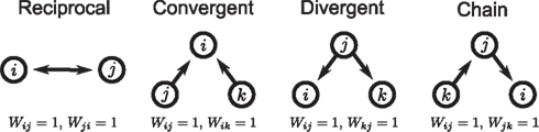
Figure 1. The four second order connection motifs of reciprocal, convergent, divergent, and chain connections.

To define the SONETs and the second order connectivity statistics more precisely, we introduce notation for the connectivity matrix W which defines the connectivity among N neurons. The component W_ij = 1 indicates a connection from neuron j onto neuron i, and W_ij = 0 if that connection is absent. In SONETs self coupling is not allowed; therefore W_ii = 0.

In this paper we consider only homogeneous networks where the probability of any combination of connections is independent of the neurons’ labels. Thus, there is only one first order connectivity statistic: the connection probability p that determines the marginal probability of the existence of any connection W_ij,

For the independent random network model the probability of any pair of connections would be p². We introduce second order connectivity statistics that measure deviations from independence among pairs of connections that share a neuron. Since the network is homogeneous, we define a single second order connectivity statistic for each motif of Figure 1. The statistics α_recip, α_conv, α_div, and α_chain specify how the probabilities of the reciprocal, convergent, divergence, and chain motifs, respectively, deviate from independence:

for any triplet of distinct neurons i, j, and k. In this way, a non-zero α yields a correlation between the connections of its corresponding motif.

The SONET model is a five-dimensional probability distribution (parametrized by p and the four α’s) for the network connectivity W that satisfies conditions (1) and (2). As the probability distribution adds minimal structure (i.e., higher order correlations) beyond these constraints, the SONET model reduces to the Erdoős–Rényi model when all α’s are zero.

For technical reasons, the SONET model only approximately satisfies the maximum entropy condition for minimal structure (Jaynes, 1957), but instead uses dichotomized Gaussian random variables analogous to those of Macke et al. (2009). The dichotomized Gaussian random variables satisfy the maximum entropy condition for continuous random variables, which are then dichotomized to be either zero or one, forming the W_ij. Hence, to generate a SONET, one simply samples a N(N − 1)-dimensional vector of joint Gaussian random variables and thresholds them into the Bernoulli random variables W_ij. The main technical challenge is calculating the covariance matrix of the joint Gaussian so that W satisfies the second order statistics (2). See (Zhao et al., in preparation) for details.

Estimating Connectivity Statistics

The above definitions of the first and second order connectivity statistics are based on a probability distribution for the connectivity matrix W. From a given network with connectivity matrix W, one can estimate these statistics directly from W. We use and to denote these descriptive statistics.

The average connectivity is simply the ratio of the number of connections N_conn present in W with the total possible: , where N_conn = ||W||₁≡Σ_i,j|W_ij|. The average second order connectivity statistics can likewise be determined by the total number of corresponding two-connection motifs that are present in the network, divided by the total possible:

where N_k for k ∈ {recip, conv, div, chain} is the number of times motif k appears in the network. The N_k can be quickly calculated from W via N_recip = Tr(W²)/2, N_conv = (||W^TW||₁−||W||₁)/2, N_div = (||WW^T||₁−||W||₁)/2, N_chain = (||W²||₁−Tr(W²), where W^T denotes matrix transpose and Tr(W) denotes trace.

In our network simulations, we compare the measured to the network synchrony even when we know the underlying probability distribution and hence the parameters α from the definition (2). Because these networks are generated probabilistically, the actual will vary slightly from α. We find that predicts synchrony better than α.

Relating Second Order Connectivity Statistics to Degree Distribution

A common method to describe network structure is through the degree distribution (Newman, 2003; Boccaletti et al., 2006). In this section we derive a relationship between the second order connectivity statistics and degree distribution. This relation will be useful in understanding the effect of the connectivity statistics and synchrony.

The in-degree of a neuron is the total number of connections directed toward a neuron, for neuron i, and the out-degree is the total number of connections directed away from the neuron, . The mean in-degree is equal to the mean out-degree, so we just refer to a mean degree.

Using the definitions (2) of α, one can calculate that the variance of the in-degree depends on α_conv, the variance of the out-degree depends on α_div, and the covariance between in-degree and out-degree depends on α_recip and α_chain:

where i is an arbitrary neuron index.

We can simplify the relationships between the α and the second order statistics of the degree distribution in the limit of large network size N. Neglecting terms that go to zero in this limit¹ and rewriting in terms of the expected mean degree E(d) = (N − 1)p, we find the following relationships between the connectivity statistics and the degree distribution:

Hence, α_conv and α_div are nearly equal to the variance of the in-degree and out-degree distributions, normalized by the mean degree squared (with a small offset 1/E(d)). α_chain is nearly equal to the covariance between in-degree and out-degree, normalized by the mean degree squared.

Generating Networks with Correlated Power Law Degree Distribution

We developed an algorithm based on the approach by Chung and Lu (2002) to generate directed networks with expected power law degree distributions with a range of second order connectivity statistics (3). We let p_d(x, y) be this degree distribution, with x = d_in and y = d_out. We set the marginal distributions of the in- and out-degrees to truncated power laws with exponentβ_i:

where the cutoff parameters satisfy 0 < a_i < b_i < N, and the normalization constants c_i and d_i are chosen to make the marginal distributions continuous at a_i and integrate to 1. Below the lower cutoff a_i, we let the distribution increase smoothly with exponent γ_i.

For a given set of networks, we fixed the right cutoff parameters b_i and the rising exponents γ_i. The left cutoff parameters a_i and the exponent β_i were then chosen for each network to match the desired average connectivity p as well as the second order connectivity statistics α_conv (for i = in) or α_div (for i = out) by numerically solving the equations [cf. (5)]

for (α_in, β_in) and analogous equations for (α_out, β_out) in terms of α_div.

To vary the correlation between in- and out-degrees and thus α_chain, we let the full degree distribution p_d(x,y) be determined by the marginal distributions p_in and p_out and a Gaussian copula with correlation coefficient ρ. In this way, we can sample from p_d(x,y) by a two step process. We generate a joint Gaussian with correlation coefficient ρ and compose each component with the cumulative distribution function of the Gaussian to obtain a sample (u, v) from the Gaussian copula. Next, we compose the result with the inverse of the cumulative distribution functions to obtain the expected in-degree and out-degree as a sample from p_d(x,y).

Finally, to generate the network, we sample N points (x_i,y_i) from p_d(x,y), which give the expected in-degree and out-degree, respectively, of each neuron i. We let the probability of each network connection W_ij from neuron j to neuron i be proportional to x_i,y_j, where the proportionality constant is chosen so that the average connectivity is Pr(W_ij = 1)=p. As described in (Chung and Lu, 2002), as long as max_i,j x_i y_j ≤N(N−1)p, this approach yields a network whose distribution of expected degrees is given by p_d(x,y). This condition was not satisfied for some networks so that their degree distribution deviated from the prescribed p_d(x,y). Since we measure the second order statistics directly from the generated connectivity matrix via (3), such deviations were not a concern.

Analysis of Complete Synchrony

To examine the influence of the second order connectivity statistics on network synchrony, we will analyze the stability of the two extreme cases of synchrony, the perfectly synchronous state and the completely asynchronous state. Through linearizations around these states, we derive conditions between the connectivity statistics and synchrony that are valid near these states. We begin by analyzing complete synchrony.

Stability of synchrony determined using master stability function

To determine the stability of the perfectly synchronous case, we linearize the equations for network dynamics around synchrony using the master stability function approach by Pecora and Carroll (1998). This approach is based on determining synchrony in a system of identical, noise-free, coupled oscillators:

where the state of oscillator i at time t is described by the vector x _i(t). The dynamics of this system are determined by the scalar coupling strength S and two vector-valued functions of the same dimension as the interval variable vector x _i: the internal dynamics function F and the coupling function H. We rewrite (8) in terms of the Laplacian matrix L = D − W, where D is the diagonal of row sums of the connectivity matrix W,

Using the master stability function approach, one can determine a critical stability region in the complex plane that is based solely on the neuron dynamics (given by F and H) and is independent of network connectivity. The influence of the network on the stability enters through the eigenvalues μ_i of L, as the eigenvalues scaled by the coupling strength Sμ_i must lie in the critical region for the synchronous state to be stable (Arenas et al., 2008).

If the neuron model is not known, it is not possible to know the critical region in the complex plane, reflecting the fact that the topology alone cannot determine whether a network will synchronize. However, a tighter spread of the eigenvalues will make it easier to scale them by S to fit within the critical region. Therefore, changes in network structure that decrease the spread of the eigenvalues will favor synchronizability. One measure of this eigenvalue spread for asymmetric matrices, as suggested by Nishikawa and Motter (2010), is the variance of the eigenvalues normalized by the mean degree squared,

where is the mean of the eigenvalues and d is the mean degree (4). This variance ignores the zero eigenvalue μ₁ = 0 present in every Laplacian matrix.

Modifications for chemical synapses

The master stability function requires the subtraction of H(x _i) in (8) to ensure that the synchronous state exists and satisfies the equation . The H(x _i) term is suitable for neuron models with electrical synapses but is not an appropriate model for chemical synapses because it implies that a connection from neuron j onto neuron i leads to an equivalent negative effect from neuron i onto itself. To model chemical synapses, we must remove the offending H(x _i) term, yielding:

The rows of the connectivity matrix W may not sum to the same value, in contrast to the Laplacian matrix L of (9) which must have rows that sum to zero. Hence, if we substitute the synchronous state , we would get different, inconsistent equations that must satisfy:

where the ith row sum of W is , the incoming degree of neuron i. If all neurons do not have the same incoming degree, then we cannot solve for independent of i and the synchronous state does not even exist.

Therefore, for chemical synaptic networks (11), rather than analyzing the stability of the synchronous state, we seek to determine how far the network is from having a synchronous solution. In the spirit of the master stability function analysis, we desire a measure of synchronizability analogous to (10) based only on network properties. We propose that network synchrony will decrease with the variance of the in-degrees, normalized by their mean squared

Connecting stability measures to network topology

Fortunately, we can merge the two normalized variances and into the same measure. It turns out that, for many large networks, the eigenvalues of the Laplacian matrix L = D − W are dominated by the diagonal entries D, which are the in-degrees If the connectivity matrix were normal (WW^T = W^TW), then this fact would follow from the Wielandt–Hoffman theorem (Hoffman and Wielandt, 1953), as this theorem shows that (with a suitable reordering of the eigenvalues μ_i)

Therefore, reproducing an argument from (Zhan et al., 2010), the relative average squared deviation is

which will tend to be small. The worst case would be when all in-degrees are the same (and equal to d), in which case the bound would be 1/d. Variation in the degrees makes the bound smaller and the eigenvalues μ_i even closer to the in-degrees .

Although our matrices W are not necessarily normal, we have observed that the eigenvalues μ_i are indeed close to the in-degrees . An example is shown in Figure 2. Thus, we infer that our two measures based on (8) and (11) are approximately equal, , and will simply use .

FIGURE 2

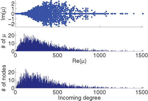
Figure 2. Comparison between the eigenvalues μi of the Laplacian and the network in-degree for a sample SONET. A scatter plot of the eigenvalues is shown in the top plot. Note that the real axis scale is much larger than the imaginary axis, so the imaginary parts of the eigenvalues are relatively small. The middle panel shows a histogram of the real parts of these eigenvalues. The histogram of the in-degrees shown at bottom closely matches that of the eigenvalues. Network statistics are: p = 0.1, N = 3000, α_recip = 0, α_conv = α_div = α_chain = 0.5.

Given (6a), we can go one step further, and connect the synchronizability measure directly with the network statistic α_conv. Comparing (6a) to (13), we see that

where we have used the mean degree d of the network as a proxy for its expected value E(d). Hence, we expect a higher frequency of the convergent connection motif to decrease synchrony.

Stability of the Asynchronous State

The emergence of synchrony

An approach to perform a similar stability analysis for the completely asynchronous state of heterogeneous, noisy oscillators has been recently developed by Restrepo et al. (2006a,b). The asynchronous state is where the oscillators are as spread out evenly as though they were uncoupled (in a sense determined by the oscillator dynamics). The analysis begins with a coupled oscillator model similar to the one used in the master stability function approach (8):

where ξ_i(t) is a noise term and the model is specified by the functions F, H, and k. One notable difference in this model is that the oscillators can be heterogeneous since their dynamics depend on the parameter vectors η_i. Two important conditions of the analysis are that the parameters cannot be correlated with the network structure and that each neuron must receive many inputs.

For the asynchronous state to be an approximate solution of this system, the factor multiplying W must be approximately zero when the neurons are asynchronous. To satisfy this condition, the equation has an extra term 〈H(x)〉, which is the average of H(x) over the oscillators when they are spread over the asynchronous state. Since 〈H(x)〉 is just a constant vector, it is less problematic than the H(x _i) of (8).

Restrepo et al. (2006a,b) analyze the coupling strength where synchrony just begins to emerge in the network (i.e., where the asynchronous state becomes unstable). Their key result is that this critical coupling strength depends on the network structure only through the largest eigenvalue λ_max of the connectivity matrix W. Clearly, this coupling strength also depends on the oscillator models and the manner in which they are coupled, but these influences are a separate factor multiplied by λ_max. Given two networks with different values of λ_max but with neurons whose dynamics are governed by the same oscillator model, synchrony will emerge at a lower coupling strength for the network with the larger λ_max. This separation of the oscillator dynamics from the network structure is in the same spirit as the master stability function analysis and allows us to incorporate λ_max into our notion of the synchronizability of the network.

Linking emergence of synchrony to network topology

Restrepo et al. (2007) also derive approximate expressions for the largest eigenvalue λ_max. If we ignore any correlation between the degrees of neighboring neurons, λ_max is a simple function of the degree distribution Given the relationship (6c) between α_chain and the covariance of the degree distribution, the maximum eigenvalue can be written in terms of α_chain:

Hence, λ_max will be nearly zero when α_chain = −1 (its minimum value) and will increase linearly with α_chain with slope equal to the mean degree.

Neuron Models

We simulated many neuron models to explore the extent to which our results were model-independent.

Kuramoto model

The Kuramoto model (Kuramoto, 1984), originally proposed by Yoshiki Kuramoto, is a network of continuously coupled oscillators with phase θ_i (modulo 2π),

where ω is the natural frequency and ξ_i(t) is white noise,

, which we scale by σ. We specify the connectivity strength S relative to the number of oscillators N and the connection probability p of the connectivity matrix W.

PRC model

The phase response curve networks are pulse-coupled networks, meaning that the effect of the pre-synaptic neuron on the post-synaptic neuron’s phase only occurs when the pre-synaptic neuron crosses the zero phase (modulo 2π), to simulate the effect of synaptic release at the time of an action potential. At the time of the action potential, the phases θ_i of the post-synaptic neurons are advanced according to their phase response curves f_i(θ_i). If a neuron fires, it is unresponsive to any other inputs it receives at that same instant, but its phase remains at θ = 0. The PRC model

uses the same parameters as the Kuramoto model, except in some simulations we allow the natural frequency ω_i to depend on neuron i. is the time of kth spike of neuron j. The shape of the phase response curve f_i is determined by choice of a_i. c(a_i) is chosen to make the maximum value of phase response curve f_i be one. We make the average of a_i be two to make PRCs that would promote synchrony in a network coupled through excitatory synapses.

Morris-Lecar model

The Morris-Lecar model is a reduced Hodgkin-Huxley like conductance based oscillator (Morris and Lecar, 1981) with two dynamic variables voltage V and channel inactivation n determined by the equations

where m_∞(V)=[1+exp((V_1/2,m−V)/k_m)]⁻¹, n_∞(V)=[1+exp((V_1/2,m−V)/k_n)]⁻¹, and τ_n(V)=exp(−0.07V−3). The neurons are coupled by synapses that include a synaptic conductance waveform every time a pre-synaptic neuron fires, with the synaptic current I_syn,i(t)=g_syn(S_i−f_i)(E_syn−V_i) determined by the pair of dynamic equations and . Our model diverges from the original Morris-Lecar model, which used Ca⁺⁺ rather than Na⁺, but essentially retains the same framework. We have also adjusted the model parameters as follows to make the resulting phase response curve look more realistic: C = 0.1 nF, g_L = 800 pS, E_L = −53.24 mV, g_Na = 1.822 nS, E_Na = 60 mV, g_K = 400 pS, E_K = −95.52 mV, V_1/2,m = −7.37 mV, k_m = 11.97 mV, V_1/2,n = −16.35 mV, k_n = 4.21 mV, E_syn = 0 mV, τ_s = 0.5 ms, and σ = 20 pA. The synaptic conductance g_syn was varied in the individual simulations.

Spike Rate Normalization Using an Integral Controller

When neurons receive different numbers of synaptic inputs, the disparity in level of synaptic drive can cause neurons to fire at different rates. In some simulations, we desired to compensate for this effect to make the neurons have similar firing rates. Rather than attempt to numerically solve for the input currents to achieve a desired firing rate, we developed an auto-tuning network by implementing an integral controller that adjusts the input current for each neuron until it fires at the desired firing rate. The controller calculates the input current for each neuron at each firing from the error between the interspike interval and that of the desired rate: e_k(j) = isi_k(j)−(desired rate)⁻¹, where isi_k(j) is the kth neuron’s jth interspike interval. For all times t during the neuron’s j + 1st interspike interval, the current to neuron k is held at the constant , where K_i is the integral feedback constant (Ogata, 2010). When neuron k spikes again, a new e_k(j + 1) is calculated and added to the sum determining I_k(t). For our purposes, we set K_i = 1, which produced long transients, but results in stable network behaviors. Simulation were run to steady state with the integral controller on and then the current values were held constant (virtually identical results were obtained when controllers were left on through the entire simulation).

Measuring Synchrony with the Order Parameter

We use a simple quantification of network synchrony, the Kuramoto order parameter, to measure synchrony in the network simulations. The measure is based on defining a phase θ_j(t) of each neuron, which ranges from 0 to 2π to indicate the relative state of the neuron through its spiking cycle. For models that are not directly based on the phase, we define the phase as the time since the previous spike, normalized by the average period over the previous five spikes.

To calculate the order parameter, we represent the phase of each neuron by a vector on the unit circle at angle θ_j(t). The population vector is the average of these unit vectors. The order parameter is the length of the population vector (Strogatz, 2000)

where i = and |·| represents the absolute value of the complex vector. The order parameter ranges between 0 and 1, with r = 1 representing perfect synchrony. The minimum value r = 0 occurs when the network is asynchronous and the phases are evenly distributed around the unit circle. However, r = 0 whenever the population is balanced around the circle, which could also occur when two or more equal clusters are evenly spread around the circle.

Since we are looking at oscillating neurons, we obtain equivalent results if we measure spike count correlation rather than synchrony. As long as one counts spikes in bins sufficiently smaller than the oscillation period, the synchrony induces spike correlations.

Results

Overview

We examine the influence of network structure on the synchrony of neuronal networks. We generate networks using the framework of SONETs which allows us to systematically vary second order connectivity statistics, which are the frequency of reciprocal, convergent, divergent, and chain connections shown in Figure 1 (see Materials and Methods). SONETs extend the commonly used Erdoős–Rényi random network model (Erdoős and Rényi, 1959), retaining the feature of adding minimal structure beyond what is required to match the connectivity statistics.

The effect of the second order connectivity statistics underlying SONETs are illustrated by the small networks of Figure 3. The networks illustrate how, if one keeps the connection probability fixed, increased convergence or divergence arises from having some neurons with large in- or out-degree, respectively (Figures 3A,B). The networks have many chains when the large in-degree neurons also have large out-degree (Figure 3D), but they have few chains when neurons with large in-degree have small out-degree and neurons with large out-degree have small in-degree (Figure 3C).

FIGURE 3

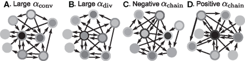
Figure 3. Illustrations of networks with different connectivity statistics. All networks contain N = 9 neurons with N_conn = 22 connections, so that the connection probability is . For each neuron, darker inner color indicates larger in-degree and darker outer color indicates larger out-degree. (A) Network with large convergence. There is large variance in in-degree. N_recip = 4, N_conv = 42, N_div = 23, and N_chain = 45 so that , , , and . (B) Network with large divergence (the same network as in panel A, but with connections reversed). There is large variance in out-degree. N_recip = 4, N_conv = 23, N_div = 42, and N_chain = 45 so that , , , and . (C) Network with few chains. Neurons with large in-degree tend to have small out-degree, and neurons with large out-degree tend to have small in-degree. N_recip = 2, N_conv = 33, N_div = 35, and N_chain = 29 so that , , , and . (D) Network with many chains. Neurons with large in-degree tend to have large out-degree. N_recip = 6, N_conv = 33, N_div = 33, and N_chain = 65 so that , , , and .

The analyses of perfect synchrony and asynchrony (see Materials and Methods) predict that two second order statistics of connectivity should play key roles in determining synchrony. First, increasing the relative frequency of the convergent connection motif (increasing α_conv) should decrease synchrony, as it pushes the network state further from complete synchrony. Second, increasing the relative frequency of the chain connection motif (increasing α_chain) should increase synchrony, as it decreases the stability of the asynchronous state.

We demonstrate in simulations that the frequency of chains and convergent motifs can influence network synchrony even when a network is not at or near the extremes of perfect synchrony and asynchrony. We present the results in four parts. First, we generate SONETs with a range of second order connectivity statistics and test the predictions of the analysis through simulations of a simple neuron model. Second, to demonstrate that these results can be explained by the analysis, we confirm that critical eigenvalue quantities from the analysis do have the predicted relationships with the network statistics. Third, to assure that our findings are not model dependent, we test networks with several different single neuron models. Fourth, we test the results with a larger range of networks to evaluate the influence of higher order network statistics on the predictions based on second order statistics.

Synchrony Determined by Second Order Connectivity Statistics

To test the effects of the second order connectivity statistics on synchrony, we generate 186 SONETs with N = 3000 neurons and 10% connectivity (p = 0.1). In addition to using the standard Erdoős–Rényi network (all α’s zero), we randomly sample the second order connectivity statistics in the ranges α_recip ∈ [−1,4], α_conv ∈ [0,1], α_div ∈ [0,1], and α_chain ∈ [−1,1]. These ranges are chosen to include the α’s used to reproduce the motif spectrum obtained from neuronal networks published by Song et al. (2005): (α_recip, α_conv, α_div, α_chain)≈(3, 0.4, 0.3, 0.2). As hinted by (6c), the valid range of α_chain depends on the α_conv and α_div (Zhao et al., in preparation). We maximize its range by sampling some networks where α_chain is set to its maximum and minimum value conditioned on α_conv and α_div.

We measure synchrony in network simulations of 3000 pulse-coupled PRC neuron models (17) in these 186 SONETs. Three example networks are shown in Figure 4. For each network, we calculate synchrony measured by the Kuramoto order parameter (19) as a function of time, and calculate its average once the network reaches steady state.

FIGURE 4

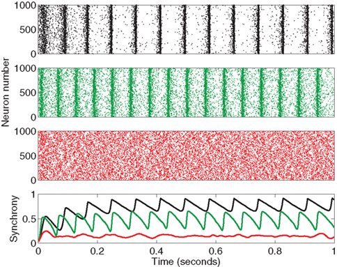
Figure 4. Sample output from the beginning of three network simulations with the PRC model (17). Top three panels are rastergrams showing the spikes of 1000 neurons (out of 3000 in each network) for the first second of time. The bottom panel shows synchrony measured by the Kuramoto order parameter (19) calculated as a function of time, where colors correspond to the associated rastergrams. The networks were chosen to illustrate the range of observed synchrony. The top network (in black) is the Erdoős-Rényi random network (α_recip = α_conv = α_div = α_chain = 0) which reached high synchrony (steady state r = 0.8). The middle network (in green) that reached moderate synchrony (r = 0.5) was generated from the second order connectivity statistics α_recip = −0.2, α_conv = 0.7, α_div = 0.6, α_chain = 0.6. The bottom network (in red) that stayed fairly asynchronous (r = 0.1) was generated from α_recip = 0.1, α_conv = 0.9, α_div = 0.9, α_chain = −0.6. For all networks, average connectivity was p = 0.1. PRC model parameters were S = 6, σ = 3, a_i = 2, and ω_i = 60 for all neurons i.

In Figure 5 the steady state synchrony is plotted against the measured second order statistics α calculated by (3). No simple relationship between any single connectivity statistic and synchrony is obvious, though it appears the Erdoős–Rényi network (black) is among the most synchronous. There appears to be a bimodal distribution of synchrony, suggesting that synchrony rapidly jumps up when some threshold is crossed.

FIGURE 5

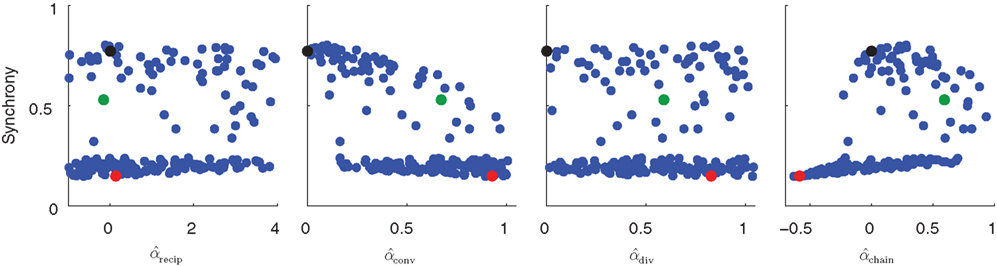
Figure 5. Scatter plots of steady state synchrony measured by the order parameter (19) as a function of individual connectivity statistics for the 186 sampled SONETs. For each panel, each dot corresponds to one network. Black, green, and red dots correspond to the networks simulated in Figure 4. Estimates of second order connectivity statistics are determined from each network connectivity matrix W via (3). PRC model parameters were S = 6, σ = 3, a_i = 2 and ω_i = 60 for all neurons i.

When synchrony is plotted against pairs of connectivity statistics, as shown in Figure 6A, the pattern of dependence on connectivity emerges. The synchrony seems to be a function of (α_conv, α_chain) alone, as the level of synchrony varies more or less smoothly in the (α_conv, α_chain) projection (lower left of Figure 6) despite the fact that α_recip and α_div are varying widely across the whole plot. For a given value of α_conv, there appears to be a threshold of α_chain above which synchrony jumps up, supporting the trend of higher synchrony with α_chain predicted by our analysis. Similarly, synchrony jumps down at a threshold value of α_conv for a given value of α_chain.

FIGURE 6

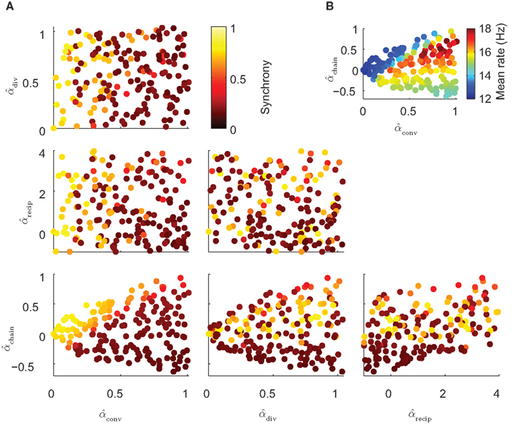
Figure 6. (A) Synchrony plotted as a function of pairs of connectivity statistics. The simulation results of the PRC model over the 186 SONETs (Figure 5) are replotted as a function of each pair of second connectivity statistics α estimated from the connectivity matrix using (3). Each dot corresponds to one network, and color indicates steady state synchrony measured by the order parameter (19). Synchrony varies smoothly in the graph with respect to α_chain and α_conv but not in the other graphs. (B) Average firing rate as a function of α_chain and α_conv for the same networks as in (A).

The connectivity statistics change the average firing rate of the network, as shown in Figure 6B. Little difference in synchrony is observed if we adjust the intrinsic frequency ω for each network to keep the average firing rate fixed (not shown). We explore below the effect of fixing not only the firing rate averaged across each network, but also making the firing rate of each neuron be the same.

Note the dependence of the valid range of α_chain on the other statistics (bottom row of Figure 6). The relationship between α_conv/α_div/α_chain and the variances/covariance of the in- and out-degree distribution shown in (6) implies that the valid range of α_chain increases with α_conv and α_div (left two panels of last row of Figure 6). The range of α_chain is also affected by α_recip (lower-right panel of Figure 6). The dependence of the range of α_chain and the other statistics creates the appearance of spurious correlations between synchrony and α_recip/α_div in the top two rows of Figure 6.

Eigenvalue Analysis

The influence of the connectivity statistics on synchrony was predicted based on analysis of eigenvalues of the network connectivity matrix W and Laplacian matrix L (see Materials and Methods). An analysis of the asynchronous state predicts synchrony will increase with the largest eigenvalue λ_max of the connectivity matrix, which should increase linearly with α_chain [see (15)]. An analysis of the synchronous state predicts synchrony will decrease as the normalized variance (10) of the Laplacian eigenvalues increases, which should be nearly equal to α_conv [see (14)].

In Figure 7, sample spectrum from a few connectivity matrices demonstrate these trends: λ_max increases with α_chain, and only α_conv modulates the variance of the eigenvalues of the Laplacian L. These observations are confirmed by the plots of λ_max and versus each connectivity statistic for the 186 generated networks (Figure 8). The right top panel shows how λ_max is nearly completely determined by α_chain according to the relationship (15) plotted in red. The second panel in the bottom row of Figure 8 shows that the normalized variance of the eigenvalues is nearly identical to the α_conv and follows the relationship (14) plotted in red. The other relationships between the eigenvalues and connectivity statistics simply reflect how the range of sampled values of α_chain depend on the other statistics, as seen in Figure 6.

FIGURE 7

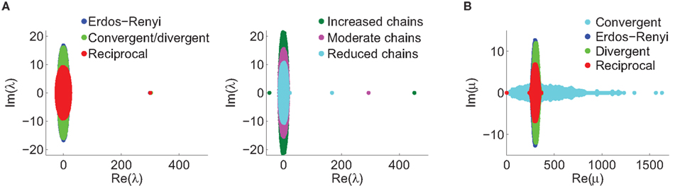
Figure 7. Spectra of connectivity matrices and Laplacian matrices for sample networks. All α’s not mentioned were zero. (A) Left: Eigenvalues for the Erdoős–Rényi network (blue) are mainly occluded by the spectra of the other matrices. Eigenvalues for convergent and divergent networks were identical. Non-zero parameters: α_conv = 0.5 (convergent), α_div = 0.5 (divergent), α_recip = 4 (reciprocal). Right: Largest eigenvalue λ_max increases linearly with α_chain. All three networks had substantial convergence and divergence (α_conv = α_div = 0.5) to allow large α_chain. Parameters: α_chain = 0.5 (increased chains), α_chain = 0 (moderate chains), α_chain = −0.4 (reduced chains). (B) Eigenvalues of the Laplacian for the networks from the left panel of A. The spread of the eigenvalues remains relatively unchanged with different frequencies of chains (not shown).

FIGURE 8

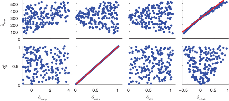
Figure 8. The distribution of key eigenvalue quantities as function of connectivity statistics for the 186 sampled SONETs. In each panel, each dot corresponds to one of the networks. Red line in top right panel is predicted dependence (15) of largest eigenvalue λ_max on α_chain. Red line in the second panel of the second row is relationship (14) between the normalized variance of the eigenvalues of the Laplacian and α_conv.

The tight relationships between α_chain and λ_max and between α_conv and confirm that the influence of these two connectivity statistics on synchrony is indeed through their influence on the key spectral properties of the connectivity matrix W and Laplacian matrix L.

Dependence of Synchrony on Single Neuron Model

The synchrony analysis, which was based around the completely synchronous and asynchronous states, predicts that the effect of topology on synchrony should be independent of the neuron model. Since these analyses were based on linearizations around those states, there is no guarantee those predictions will apply to other networks states, such as intermediate levels of synchrony. Non-linearities in neuron models could lead to model-dependent deviations from those predictions.

We test for model-dependence of the results using the three neuron models described in Methods. The simplest model is the Kuramoto oscillator (16). Second, we run additional simulations with pulse-coupled PRC oscillator models (17) under two conditions: one with noise as in Figure 6 and the other with heterogeneity in the model parameters. The third model is a simple conductance based neuronal model based on the Morris-Lecar model (18). We run all models on the above 186 SONETs and observe how synchrony is affected by changing the coupling strength.

The results shown in Figure 9 demonstrate that for each model, the influence of the network structure on synchrony is indeed determined only by α_conv and α_chain, as in each case, synchrony appears to be a function of those parameters. The relative influence of α_conv and α_chain does vary across models. For the Kuramoto model, synchrony is more strongly influenced by α_chain than α_conv (Figure 9A). For the noisy homogeneous PRC model, the result from Figure 6 is maintained at different connectivity strengths, as both convergence and chains strongly modulated the synchrony (Figure 9B). The noise-free heterogeneous PRC model has a similar dependence on the connectivity parameters (Figure 9C); replacing noise with variability across the population in intrinsic frequency and PRC shape only alters the connectivity strength at which synchrony emerges. The Morris-Lecar model (Figure 9D) has a similar dependence on α_chain and α_conv as the PRC models.

FIGURE 9

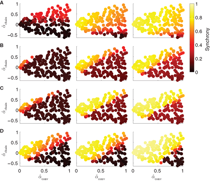
Figure 9. Dependence of synchrony on model and coupling strength. Each row corresponds to a different neuron model, and coupling strength increases with column. Panels as in Figure 6A. (A) Kuramoto model (16) with coupling strengths S = 1, 2, and 3. (B) PRC model (17) with homogeneous parameters as in Figure 5. Coupling strengths were S = 3, 6, and 9, so that middle panel is the same as lower left of Figure 6. (C) Noise-free (σ = 0) PRC model (17) with heterogeneous parameters: a_i was drawn from a Gaussian of mean 2 and SD 0.2; ω_i was drawn from a Gaussian of mean 60 and SD 6. Coupling strengths were S = 3, 6, and 9. (D) Morris-Lecar model (18) with coupling strengths g_syn set to 20, 40, and 400 pS.

In all cases, increasing α_chain or decreasing α_conv tends to increase synchrony. The increase in synchrony appears to be concentrated at an effective threshold line through the (α_conv, α_chain) plane. Whether a particular network will synchronize or not depends on many factors, but relative changes in α_conv or α_chain affect synchrony in the same way. Since the effects of changing these two connectivity statistics combine in a model-dependent manner, we obtain a two-dimensional index (α_conv, α_chain) for the synchronizability of a network.

Synchrony with Other Networks

All the above simulations were based on SONETs of N = 3000 neurons where we fixed the first order connectivity statistics (p = 0.1) and varied the second order connectivity statistics α. We did not separately manipulate higher order connectivity statistics, as the definition of SONETs does not add additional structure into the connectivity beyond that determined by the second order statistics. To explore how well α_conv and α_chain determine synchrony under a wider range of networks, we simulate networks with different first order statistics and networks with different higher order statistics.

To test the effect of changing first order statistics, we decrease the connection probability by a factor of 10 to p = 0.01. We generate 130 SONETs over the same ranges of α as the original p = 0.1 networks and simulate the PRC model of Figure 9B. As shown in the left panel of Figure 10A, the results are similar to those with p = 0.1. We also increase the network size to N = 10000 and set p = 0.03 so that the average degree p(N − 1) is approximately the same as in the original networks. Simulations from 130 SONETs demonstrate that α_conv and α_chain determine synchrony in the same manner as before (Figure 10A, right).

FIGURE 10

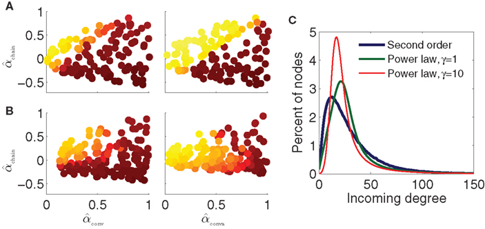
Figure 10. Dependence of synchrony on first order connectivity statistics and higher order connectivity statistics. All simulations use the PRC model and coupling strengths S = 6 of the middle panel of Figure 9B. Note that changing p or N changes the effective coupling S/(pN) in the PRC model (17). Pseudocolor scale indicates synchrony as in Figure 9. (A) SONETs with different first order statistics. Left: sparse networks with N = 3000 neurons and connection probability p = 0.01. Right: large networks with N = 10000 neurons and connection probability p = 0.03. (B) Scale-free networks with N = 3000 neurons and connection probability p = 0.01. Rising exponents of degree distribution (7) γ_in/out were set to 1 (left) and 10 (right). For left panel, the minimum attainable value of α_conv and α_div was 0.1. Maximum degrees: b_in = b_out = 300. (C) Incoming degree distributions for networks with p = 0.01 and α_conv = 0.7. The degree distributions are smoothed versions of the distribution of expected degree (7) as actual connections are generated randomly.

To manipulate higher order connectivity statistics of the network, we generate networks with power law degree distributions, i.e., with scale-free connectivity. The algorithm for generating the power law networks is described in Materials and Methods. The power law degree distribution has different higher order statistics from the degree distribution of SONETs, for fixed first (p) and second (α) order statistics. By comparing power law networks with SONETs that have the same first and second order statistics, we can evaluate the effect of the higher order statistics.

We exploit relationships (6) between the α’s and the degree distribution to generate networks across a range of second order connectivity statistics. We vary the power law exponents of the in-degree and out-degree distributions (7) independently to allow α_conv and α_div to range in (0,1). To maximize the range of α_chain, we let the correlation between in-degree and out-degree range in (−1,1).

We generate power law networks with N = 3000 neurons and average connectivity p = 0.01. We first generate 160 such power law networks where we set the rising exponents of the degree distributions (7) to γ_in = γ_out = 1 so that the degree distributions initially increase linearly as shown by the green trace of Figure 10C. Synchrony for the PRC model and these power law networks is shown in Figure 10B, left. Even for these scale-free networks, synchrony does appear to be a function of just α_conv and α_chain, as the synchrony varies smoothly in the (α_conv, α_chain) projection as before. For the most part, the same qualitative trends persist that were predicted by the synchrony analysis and were observed in the SONETs; synchrony tends to increase with α_chain and decrease with α_conv. It is clear, though, that the higher order connectivity statistics are modifying the synchrony. The synchrony pattern as a function of second order connectivity statistics in the left panels of Figures 10A,B are not identical despite the model and first order connectivity statistics being the same.

If we increase the steepness of the rise of the degree distribution by setting γ_in = γ_out = 10 (red trace of Figure 10C), the dependence of synchrony on the α changes dramatically (Figure 10B, right). Synchrony is still a function of just (α_conv, α_chain), but for larger α_conv, synchrony no longer increases monotonically with α_chain. Although the eigenvalue λ_max still has the same linear relationship (15) with α_chain, this eigenvalue no longer accurately predicts the emergence of synchrony according to the analysis of the stability of the asynchronous state.

We found large values of γ_in also lead to a non-monotonic dependence of synchrony on α_chain for other degree distribution parameters. We hypothesize that this breakdown of the asynchronous state analysis is caused by the presence of many neurons with small incoming degree. One assumption of the stability analysis of the asynchronous state is that all neurons receive many inputs. When γ_in is large, the number of neurons with small incoming degree (red trace of Figure 10C) is large enough to invalidate the analysis. The results indicate that the moderate number of neurons with even smaller incoming degree in the SONETs (blue trace of Figure 10C) does not invalidate the conclusions of the analysis.

Heterogeneity due to Convergence

Since increasing α_conv increases the variance of the in-degree distribution, neurons in networks with high α_conv will have large variability in the number of synaptic connections that they receive. This heterogeneity in the input strength will lead to heterogeneity in the firing rates across neurons in the network, thus decreasing synchrony (Chow, 1998; Denker et al., 2004). We investigate whether or not this heterogeneity is the only mechanism by which increasing α_conv decreases synchrony.

We repeat the simulation of the noisy PRC model on the SONETs (Figure 9B), where we virtually eliminate the variance in firing rates across neurons by adjusting the intrinsic frequency ω_i of each neuron to make its average firing rate be close to 10 Hz. Rather than attempting to solve for the 3000 ω_i, we use an integral controller to creating an auto-tuning network that adjusts the ω_i (see Materials and Methods, where we refer to ω more generically as an input current I). Using this approach, we can reduce the SD in the firing rate across neurons in each network to below 0.1 (compared to firing rate SD than ranged from 0.1 to upward of 10 for the high α_conv networks of Figure 9B).

As shown in Figure 11, the effect of α_conv is greatly reduced. Synchrony decreases only slightly with increased α_conv. The threshold value of α_chain where synchrony increases rapidly with α_conv depends only weakly on α_conv. The maximum value of synchrony for any α_chain does still decrease with α_conv. This residual effect of α_conv cannot be explained by its effect on the heterogeneity of firing rates, as we have eliminated that heterogeneity.

FIGURE 11

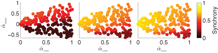
Figure 11. Dependence of synchrony on α_conv and α_chain when firing rate rate heterogeneity is eliminated. Simulations of Figure 9B were repeated where the ω_i were adjusted by an integral controller to fix the firing rate of each neuron at 10 Hz. The panels correspond to coupling strengths S=3, 6, and 9 of the PRC model (17).

Discussion

Linking Synchrony to Network Motifs

In this paper we present a framework to relate network connectivity to synchrony in homogeneous neuronal networks. We define network structure through the frequency of second order motifs, which form the basis for four second order statistics of connectivity. These second order connectivity statistics define conditional probabilities of connections between neurons, that is, how a connection from one neuron to a second neuron affects the the probability of (1) a synapse back onto the first neuron (reciprocal), (2) the second neuron receiving inputs from a third neuron (convergent), (3) the first neuron sending out connections to a third neuron (divergent), or (4) either the first neuron receiving inputs or the second neuron sending out connections (chain), as illustrated in Figure 1.

The main result of this paper is that the primary influence of second order network connectivity on synchrony is through the chain and convergent connection motifs. We obtain a two-dimensional index (α_conv, α_chain) of synchronizability that captures the effect of the network structure on the synchrony of the neuronal network. Synchrony tends to increase with the relative frequency of chains and decrease with the relative frequency of convergence, where the majority of this change in synchrony occurs abruptly along a line in (α_conv, α_chain) parameter space that depends on connectivity strength and the neuron model. There is little dependence of synchrony on divergence or reciprocal connections. The result was robust to changes in first order connectivity statistics or network size.

The value of the synchronizability index (α_conv, α_chain) stems from the fact that the influence of these network structures on synchrony was similar for a wide variety of neuron models. While there were model specific differences in the simulations, the qualitative dependency of synchrony on the proportion of chains and convergent connections in the networks was the same for most single neuron models and network models. Since the influence of chains and convergence on synchrony was predicted from linearizations around synchrony and asynchrony, it is surprising how well those statistics determined the level of synchrony over the whole range of synchrony. We expect that these linear predictions will not hold for very complicated neuron models, especially with strong coupling. The predictions did break down for networks where many neurons received few inputs, as we discovered parameter regimes where synchrony decreased with α_chain.

One result of the two-dimensional synchronizability index is that one cannot arrange networks in order of increasing synchronizability, and hence it may be impossible to predict if some network changes will increase or decrease synchrony without knowing the neuron model. If one network has both a higher α_chain and α_conv than a second network, it may be that either network may elicit higher synchrony, depending on the neuron model. For example, the Erdoős–Rényi network with all α’s zero usually synchronized better than other networks, even those with higher α_conv and α_chain. However, this trend was not model-independent, as we observed some exceptions for low connectivity strength with the Kuramoto model (Figure 9A) or when we eliminated the firing rate heterogeneity caused by positive α_conv (Figure 11).

The Decrease of Synchrony with Convergence

The decrease of synchrony with convergence is not surprising, given that the convergence is correlated with the variance of the in-degree distribution (6a) and therefore results in increased heterogeneity in firing rates. The effect of this in-degree heterogeneity can be reduced by making the synaptic strengths inversely proportional to the in-degree as done by Motter et al. (2005) or by adjusting the current to each cell so that the firing rates are the same, as we have done in our auto-tuned networks. Reducing the heterogeneity greatly reduced the effect of α_conv on synchrony but some residual effect of α_conv on synchrony remained indicating higher order effects of α_conv on synchrony that cannot be accounted for by firing rate heterogeneity alone.

At first glance, the decrease of synchrony with α_conv seems to stand in contradiction of recent results by Rosenbaum et al. (2010), where they find that the build up of synchrony in feedforward networks is primarily due to the level of convergence in the network. They show that when neurons receive many inputs (have high d_in), any small correlation among their inputs is amplified. This pooling of many inputs averages out independent fluctuations but not the correlations. Thus, increasing convergence increases correlations and synchrony. The apparent contradiction is resolved by observing that Rosenbaum et al. (2010) change the level of convergence by modifying the first order statistics of connectivity rather than the second order statistic α_conv. They do not introduce the heterogeneity of increased in-degree variance.

Independence of Synchrony from Common Input

One surprising result is that the synchronizability of a network appears to be unaffected by the relative frequency of divergent connection motifs as captured by α_div. Intuitively, one would imagine that the common input represented by the divergent connection motif would tend to synchronize neurons, as the common input leads to correlations in their inputs (Shadlen and Newsome, 1998). In feedforward networks, such correlations are amplified and can lead to synchrony in deeper layers of the network (Diesmann et al., 1999; van Rossum et al., 2002; Reyes, 2003; Tetzlaff et al., 2003; Liu and Nykamp, 2009).

To see the relationship between α_div and shared input, define β to be the fraction of shared input, i.e., the ratio between the expected number of shared connections between a pair of neurons and the expected number of connections to a single neuron. For SONETs, we can calculate from (2) how β depends on divergence

where the last approximation is in the limit of large N.

As an extreme test to see if the common input determined by α_div would lead to increased synchrony, we generated SONETs with connection probability p = 0.1 where α_div varied over its full range α_div ∈ [0, 1/p − 1] = [0, 9], leading to shared input in the range β ∈ [0.1, 1]. Such large values of α_div are not realistic, as shown by the out-degree distributions of Figure 12A. When α_div is near its maximum, the out-degrees are nearly all zero or N − 1: most neurons do not have any projections to others neurons while a small fraction (around pN) project to nearly every other neuron. Nonetheless, we wanted to test to see if such extreme cases, where neurons share almost all of their pre-synaptic connections, would lead to higher synchrony. However, as shown in Figure 12B, even large values of α_div had little influence on synchrony. An ensemble average over many networks does unmask a small increase of synchrony with α_div (not shown), but this effect is dwarfed by increases in synchrony due to α_chain.

FIGURE 12

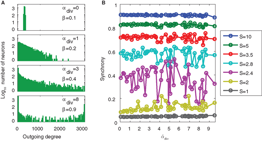
Figure 12. Demonstration of the lack of influence of divergent connections on synchrony. Each network was a SONET of N = 3000 neurons with p = 0.1 and α_recip = α_conv = α_chain = 0. (A) Sample outgoing degree distributions demonstrate how large values of α_div are unrealistic. For α_div = 8, nearly 2500 neurons have no projections and over 140 neurons project to all other neurons. (B) For each of 50 networks with different values of α_div, the PRC model (17) was simulated using 7 different coupling strengths S. Since the same networks are used, fluctuations due to the particular network structure are similar for each connectivity strength. Values of can exceed the theoretical maximum of 1/p − 1 = 9 as they are estimates from the generated connectivity matrix using (3). PRC model parameters are the same as used in Figure 9B.

For our networks, we obtain similar results if we measure spike correlations rather than synchrony (see Materials and Methods). Other researchers have also found that high common input may not necessarily lead to large spike correlations. Roxin (2011) found that changing common input by manipulating the outgoing degree distribution typically had little impact on correlations in networks of excitatory and inhibitory neurons. Renart et al. (2010) similarly showed that common input had little influence on spiking correlation, but since they used Erdoős–Rényi networks where β≈p, they could not isolate changes in common input β from changes in the first order connection probability p. Since our networks do not have inhibition, our results cannot be explained by the opposing effect of inhibition canceling out correlations in input currents (Renart et al., 2010). Instead, we are left to conclude that in these recurrent networks, as opposed to feedforward networks, common input due to divergence only weakly influences correlation, when it is not combined with convergence and chains.

The Increase of Synchrony with Chains

Instead of increasing with common input determined by α_div, synchrony increases dramatically with chains in the network. This result is consistent with the recent work by LaMar and Smith (2010), who investigated how correlation between in-degree and out-degree decreases the time until complete synchrony in noiseless pulse-coupled PRC models.

We hypothesize that the primary influence of chains is that they increase the effective coupling strength of the network. This effect can be seen by the linear dependence of the largest eigenvalue in (15). Intuitively, one can think that signals are propagated along chains in the network, so that increasing the number of chains increases the effect of the connectivity. When α_chain is large, neurons with large in-degree tend to have a large out-degree; since in this case, neurons that listen to more neurons tend to talk to more neurons, communication within the network is enhanced. Thus, synchrony emerges at a lower connectivity strength when α_chain is increased.

The analysis of the influence of chains can be extended to networks that include inhibition in order to investigate interactions within and between inhibitory and excitatory populations. We plan to study such heterogeneous SONETs to examine the effect of chains involving different patterns of excitatory and inhibitory neurons. We hypothesize that these chains will play a critical role in determining how synchrony is amplified or suppressed.

The frequency of chains in the network may have additional effects beyond the effective coupling strength that contribute to synchrony. For example the influence of chains on loops might play an additional role, as increasing α_chain increases the frequency of short loops in the network (Bianconi et al., 2008).

Higher Order Network Structure

In the SONETs, the synchronizability of the networks was determined by the second order connectivity statistics of convergence and chains. However, higher order network structure can also influence synchronizability. We introduced higher order connectivity statistics of one particular type: the additional structure contained in the power law in-degree and out-degree distributions of scale-free networks. Adding this higher order structure did alter the synchrony, even if we kept the second order connectivity statistics fixed. This simple manipulation demonstrated that knowing the second order connectivity statistics may not be sufficient to fully know the effect of the network on synchrony. Nonetheless, within a particular class of networks, we did see the same qualitative dependence of synchrony on the second order statistics, where only convergence and chains had an influence. As long as there weren’t too many neurons that received few inputs, synchrony tended to increase with chains and decrease with convergence as it did with the SONETs.

The differences observed from the in-degree distribution of the power law networks could likely be captured by adding one-third-order connectivity statistic: the probability of three connections onto a single neuron, which would presumably be linked to the skew of the in-degree distribution in analogy to (6). However, there are many more third-order connection motifs (12 in all) so that dipping into third-order statistics would greatly increase the complexity. We expect, though, that only a subset of those third-order statistics would influence synchrony.

Other higher order network statistics that have captured a lot of attention are the clustering coefficient and mean path length often examined in the context of small world networks Watts and Strogatz (1998). A number of studies have looked at the influence of network connectivity on neuronal activity and synchrony in the context of small world models (Netoff et al., 2004; Kitano and Fukai, 2007; Kriener et al., 2009). In the classical small world models, all the second order network statistics α are zero except α_recip, so one cannot observe the effect of α_conv or α_chain in these models. For the networks parameters we used, the influence of these second order statistics on synchrony was substantially larger than the influence of the small world rewiring parameter.

While the brain may have higher order connectivity statistics, there are several advantages to using second order statistics to describe a network. In general, lower order statistics require less data to estimate than do higher order statistics; it may be possible to estimate the five SONET parameters from experimental data but harder to estimate the higher order statistics. Furthermore, higher order statistics should be compared to the null hypothesis that they can be explained by the second order statistics observed. Finally, the low-dimensional framework of SONETs provides a mechanism for systematically exploring a wide range of network structures and quantifying their differences.

Conclusion

In the current study, SONETs facilitated our discovery that influence of network structure on the level of synchrony in a network of homogeneous excitatory neurons is primarily mediated through the frequency of convergent and chain connections. Given this analysis, one can predict how modification of specific connections between neurons in the network affects synchrony. By identifying the critical network structures of convergent and chain connections, one can focus efforts to identify structural changes that may play a role in enhancing or reducing susceptibility to different network states.

One application of this theory may be to understand how changes in neuronal wiring leads to pathological population activity such as abnormal synchrony. Second order statistics may provide a formalism by which to interpret changes in the network structure that may occur in a diseased state and how these changes affect network synchrony.

Conflict of Interest Statement

The authors declare that the research was conducted in the absence of any commercial or financial relationships that could be construed as a potential conflict of interest.

Acknowledgments

We thank Michael Buice, Chin-Yueh Liu, and Ofer Zeitoni for helpful discussions on the developments of the theory. We thank Alex Roxin for a careful reading of the manuscript. This research was supported by the University of Minnesota’s Grant-in-aid (Theoden Netoff and Bryce Beverlin II) and National Science Foundation grants DMS-0719724, DMS-0847749 (Duane Q. Nykamp), and CBET-0954797 (Theoden Netoff).

Footnote

1. ^If we want the expected value of the mean degree E(d)=(N−1)p to remain finite in this limit, then p must scale like 1/N, so terms such as p and Np² go to zero as N increases.

References

Abbott, L. F., and van Vreeswijk, C. (1993). Asynchronous states in networks of pulse coupled oscillators. Phys. Rev. E Stat. Phys. Plasmas Fluids Relat. Interdiscip. Topics 48, 1483–1490.

Pubmed Abstract | Pubmed Full Text | CrossRef Full Text

Arenas, A., Díaz-Guilera, A., Kurths, J., Moreno, Y., and Zhou, C. (2008). Synchronization in complex networks. Phys. Rep. 469, 93–153.

CrossRef Full Text

Axmacher, N., Mormann, F., Fernández, G., Elger, C. E., and Fell, J. (2006). Memory formation by neuronal synchronization. Brain Res. Rev. 52, 170–182.

Pubmed Abstract | Pubmed Full Text | CrossRef Full Text

Bergman, H., Feingold, A., Nini, A., Raz, A., Slovin, H., Abeles, M., and Vaadia, E. (1998). Physiological aspects of information processing in the basal ganglia of normal and parkinsonian primates. Trends Neurosci. 21, 32–38.

Pubmed Abstract | Pubmed Full Text | CrossRef Full Text

Bianconi, G., Gulbahce, N., and Motter, A. E. (2008). Local structure of directed networks. Phys. Rev. Lett. 100, 118701.

Pubmed Abstract | Pubmed Full Text | CrossRef Full Text

Boccaletti, S., Latora, V., Moreno, Y., Chavez, M., and Hwang, D.-U. (2006). Complex networks: structure and dynamics. Phys. Rep. 424, 175–308.

CrossRef Full Text

Brunel, N. (2000). Dynamics of sparsely connected networks of excitatory and inhibitory spiking neurons. J. Comp. Neurosci. 8, 183–208.

CrossRef Full Text

Cavazos, J. E., Golarai, G., and Sutula, T. P. (1991). Mossy fiber synaptic reorganization induced by kindling: time course of development, progression, and permanence. J. Neurosci. 11, 2795–2803.

Pubmed Abstract | Pubmed Full Text

Chow, C. C. (1998). Phase-locking in weakly heterogeneous neuronal networks. Physica A 118, 343–370.

Chung, F., and Lu, L. (2002). Connected components in random graphs with given expected degree sequences. Ann. Comb. 6, 125–145.

CrossRef Full Text

Denker, M., Timme, M., Diesmann, M., Wolf, F., and Geisel, T. (2004). Breaking synchrony by heterogeneity in complex networks. Phys. Rev. Lett. 92, 074103.

Pubmed Abstract | Pubmed Full Text | CrossRef Full Text

Diesmann, M., Gewaltig, M. O., and Aertsen, A. (1999). Stable propagation of synchronous spiking in cortical neural networks. Nature 402, 529–533.

Pubmed Abstract | Pubmed Full Text | CrossRef Full Text

Erdoős, P., and Rényi, A. (1959). On random graphs. I. Publ. Math. 6, 290–297.

Ermentrout, G. B., and Kopell, N. (1991). Multiple pulse interactions and averaging in systems of coupled neural oscillators. J. Math. Biol. 29, 195–217.

CrossRef Full Text

Hansel, D., Mato, G., and Meunier, C. (1995). Synchrony in excitatory neural networks. Neural Comput. 7, 307–337.

Pubmed Abstract | Pubmed Full Text | CrossRef Full Text

Hansel, D., and Sompolinsky, H. (1992). Synchronization and computation in a chaotic neural network. Phys. Rev. Lett. 68, 718–721.

Pubmed Abstract | Pubmed Full Text | CrossRef Full Text

Hoffman, A. J., and Wielandt, H. W. (1953). The variation of the spectrum of a normal matrix. Duke Math. J. 20, 37–39.

CrossRef Full Text

Holmgren, C., Harkany, T., Svennenfors, B., and Zilberter, Y. (2003). Pyramidal cell communication within local networks in layer 2/3 of rat neocortex. J. Neurophysiol. 551, 139–153.

Jaynes, E. T. (1957). Information theory and statistical mechanics. Phys. Rev. 106, 62–79.

CrossRef Full Text

Kitano, K., and Fukai, T. (2007). Variability v.s. synchronicity of neuronal activity in local cortical network models with different wiring topologies. J. Comp. Neurosci. 23, 237–250.

CrossRef Full Text

Kramer, M. A., Chang, F. L., Cohen, M. E., Hudson, D., and Szeri, A. J. (2007). Synchronization measures of the scalp electroencephalogram can discriminate healthy from alzheimer’s subjects. Int. J. Neural Syst. 17, 61–69.

Pubmed Abstract | Pubmed Full Text | CrossRef Full Text

Kriener, B., Helias, M., Aertsen, A., and Rotter, S. (2009). Correlations in spiking neuronal networks with distance dependent connections. J. Comp. Neurosci. 27, 177–200.

CrossRef Full Text

Kuramoto, Y. (1984). Chemical Oscillations, Waves, and Turbulence. Berlin: Springer-Verlag.

LaMar, M. D., and Smith, G. D. (2010). Effect of node-degree correlation on synchronization of identical pulse-coupled oscillators. Phys. Rev. E Stat. Nonlin. Soft Matter Phys. 81, 046206.

Pubmed Abstract | Pubmed Full Text | CrossRef Full Text

Lefort, S., Tomm, C., Sarria, J.-C. F., and Petersen, C. C. (2009). The excitatory neuronal network of the C2 barrel column in mouse primary somatosensory cortex. Neuron 61, 301–316.

Pubmed Abstract | Pubmed Full Text | CrossRef Full Text

Liu, C.-Y., and Nykamp, D. Q. (2009). A kinetic theory approach to capturing interneuronal correlation: the feed-forward case. J. Comp. Neurosci. 26, 339–368.

CrossRef Full Text

Macke, J. H., Berens, P., Ecker, A. S., Tolias, A. S., and Bethge, M. (2009). Generating spike trains with specified correlation coefficients. Neural Comput. 21, 397–423.

Pubmed Abstract | Pubmed Full Text | CrossRef Full Text

Morris, C., and Lecar, H. (1981). Voltage oscillations in the barnacle giant muscle fiber. Biophys. J. 35, 193–213.

Pubmed Abstract | Pubmed Full Text | CrossRef Full Text

Motter, A. E., Zhou, C., and Kurths, J. (2005). Network synchronization, diffusion, and the paradox of heterogeneity. Phys. Rev. E Stat. Nonlin. Soft Matter Phys. 71, 016116.

Pubmed Abstract | Pubmed Full Text | CrossRef Full Text

Netoff, T. I., Clewley, R., Arno, S., Keck, T., and White, J. A. (2004). Epilepsy in small-world networks. J. Neurosci. 24, 8075–8083.

Pubmed Abstract | Pubmed Full Text | CrossRef Full Text

Netoff, T. I., and Schiff, S. J. (2002). Decreased neuronal synchronization during experimental seizures. J. Neurosci. 22, 7297–7307.

Pubmed Abstract | Pubmed Full Text

Newman, M. E. J. (2003). The structure and function of complex networks. SIAM Rev. Soc. Ind. Appl. Math. 45, 167–256.

Nishikawa, T., and Motter, A. E. (2010). Network synchronization landscape reveals compensatory structures, quantization, and the positive effect of negative interactions. Proc. Natl. Acad. Sci. U.S.A. 107, 10342–10347.

Pubmed Abstract | Pubmed Full Text | CrossRef Full Text

Ogata, K. (2010). Modern Control Engineering. Boston: Prentice-Hall.

Oswald, A.-M. M., Doiron, B., Rinzel, J., and Reyes, A. D. (2009). Spatial profile and differential recruitment of GABA_B modulate oscillatory activity in auditory cortex. J. Neurosci. 29, 10321–10334.

Pubmed Abstract | Pubmed Full Text | CrossRef Full Text

Parent, J. M., Yu, T. W., Leibowitz, R. T., Geschwind, D. H., Sloviter, R. S., and Lowenstein, D. H. (1997). Dentate granule cell neurogenesis is increased by seizures and contributes to aberrant network reorganization in the adult rat hippocampus. J. Neurosci. 17, 3727–3738.

Pubmed Abstract | Pubmed Full Text

Pecora, L. M., and Carroll, T. L. (1998). Master stability functions for synchronized coupled systems. Phys. Rev. Lett. 80, 2109–2112.

CrossRef Full Text

Perin, R., Berger, T. K., and Markram, H. (2011). A synaptic organizing principle for cortical neuronal groups. Proc. Natl. Acad. Sci. U.S.A. 108, 5419–5424.

Pubmed Abstract | Pubmed Full Text | CrossRef Full Text

Renart, A., de la Rocha, J., Bartho, P., Hollender, L., Parga, N., Reyes, A., and Harris, K. D. (2010). The asynchronous state in cortical circuits. Science 327, 587–590.

Pubmed Abstract | Pubmed Full Text | CrossRef Full Text

Restrepo, J. G., Ott, E., and Hunt, B. R. (2006a). Emergence of coherence in complex networks of heterogeneous dynamical systems. Phys. Rev. Lett. 96, 254103.

CrossRef Full Text

Restrepo, J. G., Ott, E., and Hunt, B. R. (2006b). Emergence of synchronization in complex networks of interacting dynamical systems. Physica D 224, 114–122.

CrossRef Full Text

Restrepo, J. G., Ott, E., and Hunt, B. R. (2007). Approximating the largest eigenvalue of network adjacency matrices. Phys. Rev. E Stat. Nonlin. Soft Matter Phys. 76, 056119.

Pubmed Abstract | Pubmed Full Text | CrossRef Full Text

Reyes, A. D. (2003). Synchrony-dependent propagation of firing rate in iteratively constructed networks in vitro. Nat. Neurosci. 6, 593–599.

Pubmed Abstract | Pubmed Full Text | CrossRef Full Text

Rosenbaum, R. J., Trousdale, J., and Josić, K. (2010). Pooling and correlated neural activity. Front Comput Neurosci 4:9. doi: 10.3389/fncom.2010.00009

Pubmed Abstract | Pubmed Full Text | CrossRef Full Text

Roxin, A. (2011). The role of degree distribution in shaping the dynamics in networks of sparsely connected spiking neurons. Front. Comput. Neurosci. 5:8. doi: 10.3389/fncom.2011.00008

Pubmed Abstract | Pubmed Full Text | CrossRef Full Text

Shadlen, M. N., and Newsome, W. T. (1998). The variable discharge of cortical neurons: implications for connectivity, computation, and information coding. J. Neurosci. 18, 3870–3896.

Pubmed Abstract | Pubmed Full Text

Song, S., Sjostrom, P. J., Reigl, M., Nelson, S., and Chklovskii, D. (2005). Highly non-random features of synaptic connectivity in local cortical circuits. PLoS Biol. 3, e68. doi: 10.1371/journal.pbio.0030068

Pubmed Abstract | Pubmed Full Text | CrossRef Full Text

Strogatz, S. (2000). From Kuramoto to Crawford: exploring the onset of synchronization in populations of coupled oscillators. Physica D 143, 1–20.

CrossRef Full Text

Strogatz, S. H., and Mirollo, R. E. (1991). Stability of incoherence in a population of coupled oscillators. J. Stat. Phys. 63, 613–635.

CrossRef Full Text

Tetzlaff, T., Buschermhle, M., Geisel, T., and Diesmann, M. (2003). The spread of rate and correlation in stationary cortical networks. Neurocomputing 52, 949–954.

CrossRef Full Text

Uhlhaas, P. J., and Singer, W. (2010). Abnormal neural oscillations and synchrony in schizophrenia. Nat. Rev. Neurosci. 11, 100–113.

Pubmed Abstract | Pubmed Full Text | CrossRef Full Text

Van Drongelen, W., Koch, H., Marcuccilli, C., Pena, F., and Ramirez, J.-M. (2003). Synchrony levels during evoked seizure-like bursts in mouse neocortical slices. J. Neurophysiol. 90, 1571–1580.

Pubmed Abstract | Pubmed Full Text | CrossRef Full Text

van Rossum, M. C. W., Turrigiano, G. G., and Nelson, S. B. (2002). Fast propagation of firing rates through layered networks of noisy neurons. J. Neurosci. 22, 1956–1966.

Pubmed Abstract | Pubmed Full Text

Watts, D. J., and Strogatz, S. H. (1998). Collective dynamics of “small-world” networks. Nature 394, 440–442.

CrossRef Full Text

Zeng, L. H., Xu, L., Rensing, N. R., Sinatra, P. M., Rothman, S. M., and Wong, M. (2007). Kainate seizures cause acute dendritic injury and actin depolymerization in vivo. J. Neurosci. 27, 11604–11613.

Pubmed Abstract | Pubmed Full Text | CrossRef Full Text

Zhan, C., Chen, G., and Yeung, L. F. (2010). On the distributions of Laplacian eigenvalues versus node degrees in complex networks. Physica A 389, 1779–1788.

CrossRef Full Text