Bayesian population decoding of spiking neurons

- 1 Werner Reichardt Center for Integrative Neuroscience, University of Tübingen, Tübingen, Germany
- 2 Bernstein Center for Computational Neuroscience, Tübingen, Germany
- 3 Computational Vision and Neuroscience Group, Max Planck Institute for Biological Cybernetics, Tübingen, Germany
- 4 Gatsby Computational Neuroscience Unit, University College London, London, UK
Reconstructing stimuli from the spike trains of neurons is an important approach for understanding the neural code. One of the difficulties associated with this task is that signals which are varying continuously in time are encoded into sequences of discrete events or spikes. An important problem is to determine how much information about the continuously varying stimulus can be extracted from the time-points at which spikes were observed, especially if these time-points are subject to some sort of randomness. For the special case of spike trains generated by leaky integrate and fire neurons, noise can be introduced by allowing variations in the threshold every time a spike is released. A simple decoding algorithm previously derived for the noiseless case can be extended to the stochastic case, but turns out to be biased. Here, we review a solution to this problem, by presenting a simple yet efficient algorithm which greatly reduces the bias, and therefore leads to better decoding performance in the stochastic case.
1 Introduction
One of the fundamental problems in systems neuroscience is to understand how neural populations encode sensory stimuli into spatio-temporal patterns of action potentials. The relationship between external stimuli and neural spike trains can be analyzed from two different perspectives. In the encoding view, one tries to predict the spiking activity of individual neurons or populations in response to a stimulus. By comparing the prediction performance and properties of different encoding models, we can gain insights into which models are most suitable for describing this mapping. Alternatively, we can also study the inverse mapping: Given observed spike trains, we try to infer the stimulus which is most likely to have produced this particular neural response (see Figure 1). In this case, we are putting ourselves in the position of a “sensory homunculus” (Rieke et al., 1997) which tries to reconstruct the sensory stimuli given only information about the activity of single neurons or a neural population. By studying what properties of the stimulus can be decoded successfully, we gain insight into the features of the stimulus that are actually encoded by the population.
FIGURE 1
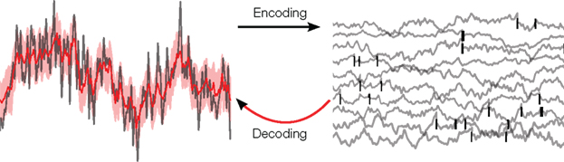
Figure 1. Illustration of the decoding problem: A time varying stimulus (left side, gray) is mapped or encoded into a set of spikes occurring at distinct points in time (right side, black bars). In our study, these time-points are assumed to originate from threshold crossings of an underlying membrane potential (right side, gray). The decoding problem consists of reconstructing the stimulus on the basis of the spike times only. This leads to an estimate of the stimulus (left side, red) and, in a probabilistic setting, also to an uncertainty estimate (left side, red shaded region).
In addition to decoding external stimuli from spike trains, decoding other endogenous signals can be of interest, since, they are thought to influence spiking activity, and should thus be represented in the population activity. For example, Montemurro et al. (2008) and Rasch et al. (2008) investigated how well local-field potentials could be decoded from the spike trains of neurons in striate visual cortex.
The general problem of decoding stimuli from spike trains can be challenging: First, the mapping of stimuli to the spike trains of single neurons (the encoding model) might be an unknown, complicated, non-linear transformation. Second, the nature of the relationship may change dynamically over time. However, even if we assume the encoding model to be known, fixed and relatively simple, decoding is not a trivial problem, because the mapping between stimuli and spike trains is not deterministic. This means that, even if the same stimulus was presented multiple times under identical conditions, it would not result in the same spike trains. Neural responses are variable because variations in channel-openings and other cellular processes lead to variations in their response even to identical stimuli (Faisal et al., 2008). Additional variability arises from the population sensitivity to influences other than the stimulus chosen by the experimenter. For example, even if the same visual stimulus is presented to a neuron in visual cortex, its spiking activity can be influenced by the behavior of the animal or mental states such as attention.
Another complication for decoding is that spike trains of neurons consist of discrete events, whereas sensory signals (or other signals of interest may) change continuously in time. Therefore, the discreteness of neural spikes implies constraints on what properties of the stimulus can be successfully reconstructed. For example, if neurons have low firing rates, then it may be impossible to resolve very high-frequency information in their inputs (Seydnejad and Kitney, 2001; Lazar and Pnevmatikakis, 2008). The discrete nature of spike trains requires additional assumptions about the properties of the stimulus, such as smoothness or other band-width limitations, similar to the Nyquist theorem.
In a recent study (Gerwinn et al., 2009), we investigated decoding schemes for spike trains generated by a known encoding model: The leaky integrate and fire neuron (Burkitt, 2006). The dynamical properties of this popular neuron model have been studied extensively (Fourcaud and Brunel, 2002). Importantly, it allows for precise spike timing which has been shown to carry information about the temporal (Borst and Theunissen, 1999) as well as spatial aspects (Panzeri, 2001) of dynamic stimuli. Many previous studies on stimulus reconstruction, however, mainly focused on the reconstruction of stimuli from spike counts only. A classic example is the population vector method for decoding movement directions (Georgopoulos et al., 1982). For the leaky integrate and fire neuron the encoding into spikes may seem to be linear, as the input is accumulated linearly. However, the reset when reaching a threshold renders the encoding non-linear. Therefore, a linear decoder is not the optimal decoder for this neuron model.
Starting from the noiseless encoding of leaky integrate and fire neurons, we review the non-linear decoding scheme presented in Seydnejad and Kitney (2001), Lazar and Pnevmatikakis (2008). With this decoding scheme, stimuli can be reconstructed perfectly provided that sufficiently many spikes have been observed and that we can make certain assumptions about the stimulus smoothness. To be more realistic, the model can be rendered stochastic and hence the spike timing precision is varied by allowing the threshold to be noisy rather than fixed. For this model with a noisy spike generation process, we also have to adapt the decoding model accordingly. When interpreted probabilistically, regularity assumptions such as stimulus band-width limitations turn into assumptions about stimulus likelihood. That is which stimuli are more likely than others. Observing spikes then leads to a reduction (or an increase) of the probability with which a stimulus has been presented according to how likely the observed spike train could have been produced by each stimulus.
The decoding algorithm for the deterministic case can not simply be used in the stochastic case, as it suffers from a systematic bias (Pillow and Simoncelli, 2003). Even if infinitely many spikes had been observed, applying the modified decoding algorithm would lead to a different stimulus estimate than the one which was used to generate the neural response. We showed that under some idealized assumptions this bias can be calculated and hence eliminated. Although these assumptions are unlikely to rigorously hold, empirically they still lead to a substantial reduction in bias. Finally, we will discuss alternative decoding approaches, in particular those based on generalized linear models (GLMs; Plesser and Gerstner, 2000; Paninski et al., 2007; Cunningham et al., 2008).
2 Noiseless Encoding and Decoding
Given an encoding model, we can aim to “invert” this model for decoding, and thus perform optimal decoding. We assume that the encoding model is known, and, concretely, assume that it is a leaky integrate and fire neuron model (Tuckwell, 1988; Burkitt, 2006; see Box). This encoding model is illustrated on the right-hand side of Figure 2.
Leaky integrate and fire neuron
The neuron model consists of a membrane potential Vt which evolves over time according to the following differential equation:

where It is the input signal which is accumulated. τ is a time constant and specifies the leak term. Whenever Vt reaches a predefined threshold θ, the potential is reset to Vreset and a spike is released. The solution to this equation can be found to be:
where t− is the time of the last reset (spike). Without loss of generality, we assume the reset potential Vreset to be zero. From this solution, we see that the stimulus It is convolved with an exponential filter exp (−τ) and integrated (see also Figure 2).
FIGURE 2
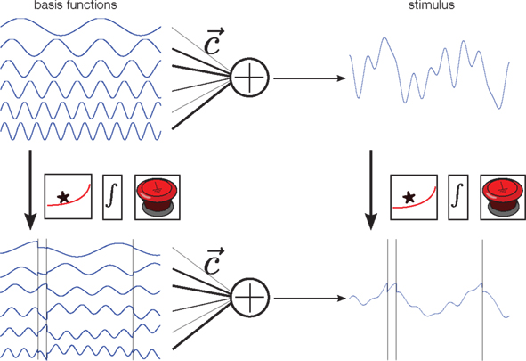
Figure 2. Illustration of the encoding process. Each stimulus is constructed by first drawing random weights c from a Gaussian distribution, and then forming a weighted superposition of basis functions with these weights (top row). This generates a new smooth stimulus on each trial. In our neuron model, the membrane potential at any time is a “leaky” integral of the stimulus. Thus, the membrane potential can be calculated by convolving the stimulus with an exponential filter (first box). Whenever the resulting integrated signal (second box) reaches a predefined threshold the integration is reset (third box). Alternatively, one can apply the filtering, integrating and resetting at the given spike times to each basis function separately, and then do a weighted summation of these signals. Both constructions lead to the same membrane potential, and thus the same spike trains.
In addition to the encoding model, we also need a representation or parametrization of the stimulus. We assume that the stimulus can be represented by a weighted superposition of a fixed number of basis functions (Figure 2, upper left). Therefore, each stimulus is a smooth function, but one which can be uniquely described using the set of weights that were used to generate it. In this way, prior knowledge (or assumptions) can nicely be translated into prior distributions over coefficients. For example, if the Fourier basis is chosen as basis function set, a “one over f” prior can easily be incorporated by a properly defined Gaussian distribution over coefficients, for which the variance of higher frequencies decreases proportionally to the inverse of the frequency.
Importantly, the operations that map the stimulus onto the membrane potential (filtering, integration, and reset at the spikes times) can also be applied to each basis function individually. Superimposing these modified basis functions with the same weightings results in the same membrane potential. In addition, we know that at the spike time-points, the value of the membrane potential equals the threshold. As the membrane potential is obtained by a weighted sum of the modified basis functions, this equality constraint defines a set of linear equations that we want to solve for the unknown coefficients of the basis functions (Seydnejad and Kitney, 2001; Lazar and Pnevmatikakis, 2008). Thus, observing as many interspike intervals as basis functions results in a perfect reconstruction of the stimulus1. Note that these linear constraints can only be obtained for the modified basis functions, not directly for the stimulus.
For the case of only two basis functions we have illustrated the constraints defined by two interspike intervals in Figure 3. For the first interspike interval the membrane potential has to fulfill the constraint of being at the reset potential at the beginning of the interval and at the threshold at the end of it. This restricts the possible stimuli to a linear subspace shown as a green line in the upper part of Figure 3A. A similar restriction results from the second interspike interval leading to the linear subspace plotted in red. The true coefficients c* that were used to generate the stimulus, therefore have to be at the intersection of these two constraint subspaces. In the case of underdetermined, i.e., uncertain stimulus reconstruction, there are more constraints which could be exploited. As can be seen in Figure 3, there are some coefficients which fulfill the threshold constraint but result in membrane potentials which cross the threshold between spikes. Incorporating these constraints into a decoding procedure is computationally more demanding, as in each time bin they only define an inequality constraint. Solving this would result in a linear program with as many constraints as there are time bins, which would be computationally infeasible in almost all interesting cases. For the example in Figure 3, we plotted the space of solutions, which additionally account for the inequality constraints in subplot B. Neglecting these constraints, we need possibly more observations, but are still able to reconstruct the stimulus perfectly eventually: The linear constraints implied by the observed spikes will eventually “rule out” all stimuli which violate one of the inequality constraints.
FIGURE 3
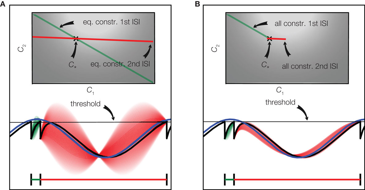
Figure 3. Spikes imply linear constraints on the stimulus. (A) Equality constraints only: The stimulus (blue) consists of a superposition of two basis function (one sine and one cosine function). The resulting membrane potential is plotted in black. Whenever the potential reaches the threshold (gray) a spike is fired. The linear constraint originating from the equality constraints of the first interspike interval are plotted in green in the upper plot. A discrete set of points along this linear constraint are selected and the corresponding membrane potentials are plotted in green in the lower plot. The same is shown for the second interspike interval in red. The perfect reconstruction of the stimulus (coefficients) is found by the intersection of the linear constraints. The brightness of the background indicates the probability of each pair of coefficients according to the prior distribution. (B) Equality and inequality constraints: The same configuration as in (A) is plotted, but additionally the inequality constraints imposed by the period of silence between spike times are taken into account as well. This results in a smaller subspace of possible solutions as shown in the upper plot.
If fewer interspike intervals than basis functions have been observed, the linear system which is defined by the threshold constraints is underdetermined. This means that multiple reconstructions are consistent with the equality constraints, and one can freely choose an estimate within the solution space. One principle for choosing a single one under all possible solutions (for example along the green line in Figure 3, if only the first interspike interval had been observed) is to take the one with minimal norm, i.e., the one for which the sum of the squares of the coefficients is minimal. This construction will always yield a reconstruction which is consistent with the spike times observed, but not necessarily one which is also consistent with the observed silence periods. This particular choice of reconstruction also has a probabilistic interpretation: It corresponds to the mean of a Gaussian distribution, which is obtained from constraining a Gaussian prior distribution (indicated by the background brightness in Figure 3) over coefficients to the subspace spanned by the linear constraints. However, ignoring the inequality constraints and just restricting the Gaussian prior to the space of linear system solutions might result in a substantial estimate offset (even on average). Picking the solution with minimal amplitude also corresponds to a least squares solution to the equality constraints. Therefore, it is also called the pseudo-inverse (Penrose, 1955) as it can be applied in both over- and underdetermined cases. Minimal amplitude, however, might not be desirable as it biases the solution toward zero, which would not be justified if the inequalities had been taken into account.
3 Including Noise: Probabilistic Treatment
In the previous section we assumed a fixed threshold which must reached to fire a spike. Thus, there was no noise in the model, and the mapping from stimuli to spikes is deterministic. To make the model more realistic, we assume that the membrane potential is not fixed, but rather varies randomly from spike to spike (Jolivet et al., 2006). There are several possibilities, to allow for a varying threshold. First, one could add random fluctuations to the threshold, or equivalently to the membrane potential. Second, one could adapt the spike generation by generating a spike probabilistically according to the membrane potential distance to the threshold. We here assume that the threshold is drawn from a known distribution every time a spike is released. Reconstructing the stimulus, however, is then complicated by the fact that the membrane potential value is not directly observed. Thus, we no longer have equality constraints, but rather average over all possible thresholds that the membrane potential possibly could have reached. A simple solution to circumvent this problem is to apply the same decoding algorithm as above but with the equality constraint for the fixed threshold being replaced by the mean threshold rather than the actual value. However, this procedure might be problematic as the modified basis functions are calculated based on spike times, which correspond to reaching thresholds that differ from the mean threshold.
By varying the threshold every time a spike is fired, we have introduced a noise source. This readily leads to a probabilistic interpretation of the encoding task: Fixing a specific stimulus, or equivalently a vector of coefficients, results in a probability distribution over spikes times induced by the varying threshold. After having specified a prior distribution over stimuli, the distribution over spikes times can be inverted by Bayes rule to give a distribution over possible stimuli having produced an observed set of spikes, called the posterior. The posterior assigns each stimulus a probability with which it could have produced the observed neural response. The substitution of the actual value with the mean threshold for the equality constraint can also be interpreted as a Gaussian approximation to the true distribution over stimuli (Gerwinn et al., 2009). We will refer to this approximation as the Gaussian factor approximation as it essentially approximates a likelihood factor (corresponding to a single observation) with a Gaussian factor. Unfortunately, the mean of this approximation does not converge to the true stimulus, i.e., this decoding algorithm is asymptotically biased. Even if infinitely many spikes had been observed, the mean of the estimated stimulus distribution would in general be different from the true one.
To analyze the situation, it is instructive to split the stimulus, or rather the coefficient vector which describes the stimulus (see Figure 2), into two parts: one amplitude component, which determines the “size” of the stimulus, and an angular component, which represents its direction in space. The difference between estimate and true coefficients could be due to a difference in amplitude or due to a difference in orientation (or both). If, for the moment, we assume that there is no difference on average for the orientation, we can analytically calculate the bias in the radial (amplitude) component. Once we know this average amplitude difference, we can correct for it by multiplying the estimate by its inverse.
In Figure 4 we illustrate the difference between the three distributions in the one- dimensional case: the true distribution over stimuli, the Gaussian approximation without any bias correction and the Gaussian approximation with the inverse bias multiplication. In the one-dimensional case, there is only one orientation, so our assumption of the orientation being correctly estimated is trivially true. Therefore, in the one-dimensional case, the bias can be completely eliminated. Note that the elimination of the bias only implies that the estimated stimulus (mean of the distribution plotted in Figure 4) will eventually converge to the true stimulus. For a finite number of spikes and a specific stimulus (the case that is plotted in Figure 4) there is no guarantee that the distribution is close to the true posterior distribution. Nevertheless, we can see that the mean of the bias corrected version is much closer to the true mean than the uncorrected version.
FIGURE 4
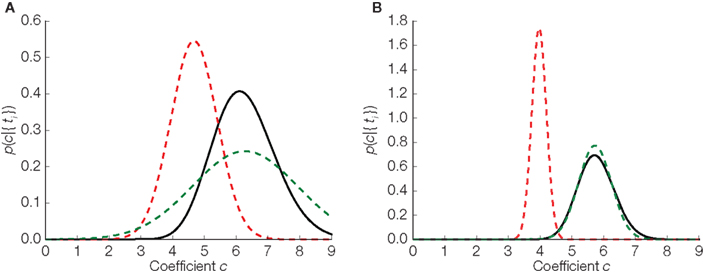
Figure 4. Replacing noisy thresholds by the mean threshold induces a bias in the stimulus estimate. Three estimators in two different situations are plotted. (A) Corresponds to the case where 10 interspike intervals have been observed. In (B) the same is shown for 40 observations. The true distribution is plotted in black, the Gaussian approximation in dashed red, and the bias corrected version of the Gaussian approximation is shown in dashed green.
To illustrate the Gaussian approximation, we analyze the equality constraint obtained from the spikes times in some more detail. Mathematically, the equality constraint is given by the equation:
where θ is the threshold and  are the modified basis functions from Figure 2, evaluated at the current spike ti. In the noiseless case, the value of the threshold is known. Therefore (1) constitutes a set of linear systems and can be solved for c with standard methods. The Gaussian approximation corresponds to replacing the threshold θ by the mean threshold plus additive Gaussian noise, which is assumed to be independent to the observation
  . The main source of the bias for the Gaussian approximation comes from this independence assumption: We know that equation (1) has to hold exactly, that is, the realization of the noise shapes the observation
  and therefore they cannot be independent. To calculate the resulting length bias, we had to assume that there is no bias for the orientation. Although this is not guaranteed to be correct in practice, this assumption empirically reduces the bias substantially, see Figure 5.
FIGURE 5
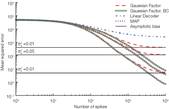
Figure 5. Our length correction substantially reduces the bias in decoding. Three different noise levels are considered here. The noise level is specified by the variance of the thresholds drawn at spike times. The larger the noise level the more prominent is the asymptotic bias (solid black lines) for the Gaussian approximation without the length bias correction (red, dashed). As a reference the performance of the linear decoder (dot-dashed blue) and the maximum a posteriori (MAP, dotted) are also plotted.
4 Alternative Decoding Schemes
So far, we have used the equality constraint to approximate the likelihood of observing the set of spikes, given the stimulus. This in turn enabled us to construct a probability over stimuli conditioned on the observations. Instead of using this approximation, we could have used one of the following alternatives:
Approximate Maximum a Posterior Estimation
The Gaussian factor approximation used previously was obtained by assuming independence of the indirect observation of the modified basis functions and the threshold. Under this assumption, we could replace the actual threshold value by its mean. If we do not assume this independence but still only use the fact that the membrane potential has to reach an unknown threshold whose distribution is known, we can derive another approximation of the likelihood. In this case, the mean stimulus cannot be calculated analytically. However, the most likely stimulus (maximum a posteriori estimate) can still be found by using gradient based optimizers. This procedure results in an algorithm very similar to the one presented by Cunningham et al. (2008). In Figure 5 we show the (asymptotic) performance of this estimator against the Gaussian approximation. This decoder shows very similar performance to our Gaussian factor approximation, but requires one to solve an optimization problem for each stimulus estimate.
Exact Probabilistic Decoding
Instead of approximating the likelihood function, we could try to use the exact form, without neglecting any constraints imposed by the observation of spikes. For the case of a continuously varying threshold, which is equivalent to additive noise to the membrane potential, algorithms for evaluating the likelihood have been presented by Paninski et al. (2004), see also Paninski et al. (2008). However, the associated optimization routines are computationally very demanding, because evaluating the true likelihood requires to average each of the equalities and inequalities over all possible threshold values. For other neuron models, like the GLM, for which the likelihood is given analytically, exact, and efficient decoding algorithms exists, see Ahmadian et al. (2011).
Escape Rate Approximation
The difficulty in computing the likelihood of a spike train for the leaky integrate and fire neuron model arises primarily from the hard threshold used in the model. Therefore, a potential remedy is to approximate the model by one with a probabilistic, “soft” threshold, and for which decoding is easier. In particular, GLMs are possible candidates, as inference over stimuli or parameters can be done efficiently. The corresponding decoding algorithms are either based on the Laplace ( saddle point) approximation (Paninski et al., 2007; Lewi et al., 2009) or on Markov Chain Monte Carlo methods (Ahmadian et al., 2011; Pillow et al., 2011). Such approximations of the leaky integrate and fire model based on GLMs are known as escape rate approximations (Plesser and Gerstner, 2000). The key assumption is that the probability of observing a spike at a particular point in time depends only on the current value of the integrated membrane potential.
Linear Decoding
A very popular decoding algorithm which does not use the information about an explicit encoding model is the linear decoder (Bialek et al., 1991; Rieke et al., 1997). A reconstruction is obtained by a superposition of fixed filters shifted to be centered at the observed spike times. The exact form of such a filter depends on the encoding model, and can be learned from stimulus–spike train pairs. There is, however, no guarantee that the linear decoder will eventually converge to the true stimulus.
5 Discussion
Decoding stimuli from sequences of spike-patterns generated by populations of neurons is an important approach for understanding the neural code. Two challenges associated with this task are that continuous stimuli or inputs are sampled only at discrete points in time, and that the neural response can be noisy. When we incorporate noise, the decoding problem naturally turns into a probabilistic estimation problem: We want to estimate a distribution over stimuli which is consistent with the observed spike trains. In our case, we assumed that the encoding model is known, and given by a leaky integrate and fire neuron model. Thus, decoding the stimuli requires inferring the mapping from spikes to stimuli, while properly accounting for the noise in the observed spike trains.
Previous studies mostly investigated the static case, in which the decoding has to be done on the basis of an estimated rate at one instant of time (Georgopoulos et al., 1982; Seung and Sompolinsky, 1993; Panzeri et al., 1999). For single spike based decoding, expressions can be obtained for different neuron models (inhomogeneous Poisson – Huys et al., 2007; Natarajan et al., 2008, GLM – Brown et al., 1998; Paninski et al., 2007; Lewi et al., 2009, and integrate and fire neurons – Bruckstein et al., 1983; Twum-Danso and Brockett, 2001; Rossoni and Feng, 2007), although most of them can only be obtained via gradient based optimization. Pfister et al. (2009) derived equations for approximately decoding continuous-valued inputs from linear–non-linear Poisson neurons, and showed that decoding the pre-synaptic membrane voltages from spike times yields update-equations for synaptic parameters which resemble known short term synaptic plasticity rules. Here, we reviewed an alternative Bayesian decoding scheme based on the linear constraint observation by Seydnejad and Kitney (2001), which does not need any optimization procedure. This Gaussian factor approximation can also be formulated in an online spike-by-spike update rule, in which the stimulus reconstruction can be updated whenever a new spike is observed (Gerwinn et al., 2009).
Above, we assumed that neurons are influenced only by the stimulus, but not by the activity of other neurons in the population. In other words, we can trivially extend the decoding scheme to the population case, if we assume that the neurons are “conditionally independent given the stimulus.” Importantly, this assumption can be relaxed easily, such that the decoding algorithm can also be applied to populations in which the neurons directly influence the spike-rates of each other. Specifically, we can also allow each spike of a neuron to generate a post-synaptic potential in any other neuron within the modeled population. As long as the form of the caused potential is known, every spike just adds a basis function with known coefficients to the indirect observations. In this way, we could analyze the effect of correlations on the decoding performance (Nirenberg and Latham, 2003).
Furthermore, the decoding scheme not only yields a point estimate of the most likely stimulus, but also an estimate of the uncertainty around that stimulus. Having access to this uncertainty allows one to optimize encoding parameters such as receptive fields in order to minimize the reconstruction error or to maximize the mutual information between stimulus and neural population response. In this way it becomes possible to extend unsupervised learning models such as independent component analysis (Bell and Sejnowski, 1995) or sparse coding (Olshausen and Field, 1996) to the spatio-temporal domain with spiking neural representations. Alternatively, we can use the presented algorithm to find a set of encoding parameters, which is optimized for reconstruction performance.
Conflict of Interest Statement
The authors declare that the research was conducted in the absence of any commercial or financial relationships that could be construed as a potential conflict of interest.
Acknowledgments
This work is supported by the German Ministry of Education, Science, Research and Technology through the Bernstein award to Matthias Bethge (BMBF, FKZ:01GQ0601), and the Max Planck Society. Jakob H. Macke was supported by the Gatsby Charitable Foundation and the European Commission under the Marie Curie Fellowship Programme. We would like to thank Philipp Berens, Alexander Ecker, Fabian Sinz, and Holly Gerhard for discussions and comments on the manuscript.
Key Concepts
the process of reconstructing the stimulus from the spike times of a real neuron or theoretical neuron model.
A neuron model which describes how a neuron will generate spikes in response to a given stimulus.
Mathematical theorem which outlines the conditions under which a stimulus with limited frequency range can be perfectly reconstructed from discrete measurements.
A formula which specifies how likely a given spike train is given a stimulus. The likelihood depends on both the encoding model and the noise model.
Average difference between the true stimulus and the reconstructed stimulus. A decoder with small bias will usually be preferable to a decoder with large bias.
Prior assumptions or knowledge about the stimuli, which are encoded in a probability distribution over possible stimuli.
A probability distribution which determines which stimuli are consistent with a given spike train: Stimuli which are consistent with the spike train have high posterior probability.
A simple yet powerful decoding algorithm which reconstructs the stimulus as a superposition of fixed waveforms centered at spike times.
Footnote
- ^Interspike intervals, not only the time of the last spike are needed, because the start point for the integration (last reset) has to be known as well.
References
Ahmadian, Y., Pillow, J., and Paninski, L. (2011). Efficient Markov chain Monte Carlo methods for decoding neural spike trains. Neural Comput. 23, 46.
Bell, A. J., and Sejnowski, T. J. (1995). An information–maximization approach to blind separation and blind deconvolution. Neural Comput. 7, 1129.
Bialek, W., Rieke, F., de Ruyter van Steveninck, R. R., and Warland, D. (1991). Reading a neural code. Science 252, 1854.
Borst, A., and Theunissen, F. E. (1999). Information theory and neural coding. Nat. Neurosci. 2, 947.
Brown, E. N., Frank, L. M., Tang, D., Quirk, M. C., and Wilson, M. A. (1998). A statistical paradigm for neural spike train applied to position prediction from ensemble firing patterns of rat hippocampal place cells. J. Neurosci. 18, 7411.
Bruckstein, A. M., Morf, M., and Zeev, Y. Y. (1983). Demodulation methods for an adaptive neural encoder model. Biol. Cybern. 49, 45.
Burkitt, N. (2006). A review of the integrate-and-fire neuron model: I. Homogeneous synaptic input. Biol. Cybern. 95, 1.
Cunningham, J. P., Shenoy, K. V., and Sahani, M. (2008). “Fast Gaussian process methods for point process intensity estimation,” in Proceedings of the 25th International Conference on Machine Learning (New York, NY: ACM), 192.
Faisal, A. A., Selen, L. P. J., and Wolpert, D. M. (2008). Noise in the nervous system. Nat. Rev. Neurosci. 9, 292.
Fourcaud, N., and Brunel, N. (2002). Dynamics of the firing probability of noisy integrate-and-fire neurons. Neural Comput. 14, 2057.
Georgopoulos, A. P., Kalaska, J. F., Caminiti, R., and Massey, J. T. (1982). On the relations between the direction of two-dimensional arm movements and cell discharge in primate motor cortex. J. Neurosci. 2, 1527.
Gerwinn, S., Macke, J. H., and Bethge, M. (2009). Bayesian population decoding of spiking neurons. Front. Comput. Neurosci. 3:21. doi: 10.3389/neuro.10.021.2009
Huys, Q. J. M., Zemel, R. S., Natarajan, R., and Dayan, P. (2007). Fast population coding. Neural Comput. 19, 404.
Jolivet, R., Rauch, A., Lüscher, H. R., and Gerstner, W. (2006). Predicting spike timing of neocortical pyramidal neurons by simple threshold models. J. Comput. Neurosci. 21, 35.
Lazar, A. A., and Pnevmatikakis, E. A. (2008). Faithful representation of stimuli with a population of integrate-and-fire neurons. Neural Comput. 20, 2715.
Lewi, J., Butera, R., and Paninski, L. (2009). Sequential optimal design of neurophysiology experiments. Neural Comput. 3, 619.
Montemurro, M. A., Rasch, M. J., Murayama, Y., Logothetis, N. K., and Panzeri, S. (2008). Phase-of-firing coding of natural visual stimuli in primary visual cortex. Curr. Biol. 18, 375.
Natarajan, R., Huys, Q. J. M., Dayan, P., and Zemel, R. S. (2008). Encoding and decoding spikes for dynamic stimuli. Neural Comput. 20, 2325.
Nirenberg, S., and Latham, P. E. (2003). Decoding neuronal spike trains: how important are correlations? Proc. Natl. Acad. Sci. U.S.A. 100, 7348.
Olshausen, B. A., and Field, D. J. (1996). Emergence of simple-cell receptive field properties by learning a sparse code for natural images. Nature 381, 607.
Paninski, L., Haith, A., and Szirtes, G. (2008). Integral equation methods for computing likelihoods and their derivatives in the stochastic integrate-and-fire model. J. Comput. Neurosci. 24, 69.
Paninski, L., Pillow, J., and Lewi. J. (2007). Statistical models for neural encoding, decoding, and optimal stimulus design. Prog. Brain Res. 165, 493.
Paninski, L., Pillow, J., and Simoncelli, E. P. (2004). Maximum likelihood estimation of a stochastic integrate-and-fire neural encoding model. Neural Comput. 16, 2533.
Panzeri, S. (2001). The role of spike timing in the coding of stimulus location in rat somatosensory cortex. Neuron 29, 769.
Panzeri, S., Treves, A., Schultz, S., and Rolls, E. T. (1999). On decoding the responses of a population of neurons from short time windows. Neural Comput. 11, 1553.
Penrose, R. (1955). “A generalized inverse for matrices,” in Proceedings of the Cambridge Philosophical Society, Vol. 51 (Cambridge: Cambridge University Press), 406.
Pfister, J., Dayan, P., and Lengyel, M. (2009). “Know thy neighbour: a normative theory of synaptic depression,” in Advances in Neural Information Processing Systems 22, eds Y. Bengio, D. Schuurmans, J. Lafferty, C. K. I. Williams, and A. Culotta (Cambridge, MA: MIT Press), 1464.
Pillow, J., Ahmadian, Y., and Paninski, L. (2011). Model-based decoding, information estimation, and change-point detection techniques for multineuron spike trains. Neural Comput. 23, 1.
Pillow, J., and Simoncelli, E. P. (2003). Biases in white noise analysis due to non-Poisson spike generation. Neurocomputing 52, 109.
Plesser, H. E., and Gerstner, W. (2000). Noise in integrate-and-fire neurons: from stochastic input to escape rates. Neural Comput. 12, 367.
Rasch, M. J., Gretton, A., Murayama, Y., Maass, W., and Logothetis, N. K. (2008). Inferring spike trains from local field potentials. J. Neurophysiol. 99, 1461.
Rieke, F., Warland, D., van Steveninck, R. R., and Bialek, W. (1997). Spikes: Exploring the Neural Code. Cambridge, MA: MIT Press.
Rossoni, E., and Feng, J. (2007). Decoding spike train ensembles: tracking a moving stimulus. Biol. Cybern. 96, 99.
Seung, H. S., and Sompolinsky, H. (1993). Simple models for reading neuronal population codes. Proc. Natl. Acad. Sci. U.S.A. 90, 10749.
Seydnejad, S. R., and Kitney, R. I. (2001). Time-varying threshold integral pulse frequency modulation. IEEE Trans. Biomed. Eng. 48, 949.
Tuckwell, H. C. (1988). Introduction to Theoretical Neurobiology. Cambridge: Cambridge University Press.
Keywords: decoding, spiking neurons, Bayesian inference, population coding, leaky integrate and fire
Citation: Gerwinn S, Macke JH and Bethge M (2011) Reconstructing stimuli from the spike times of leaky integrate and fire neurons. Front. Neurosci. 5:1. doi: 10.3389/fnins.2011.00001
Received: 12 August 2010;
Paper pending published: 10 December 2010;
Accepted: 03 January 2011;
Published online: 23 February 2011.
Edited by:
Klaus R. Pawelzik, University of Bremen, GermanyReviewed by:
Klaus R. Pawelzik, University of Bremen, GermanyLiam Paninsky, Columbia University, USA
Copyright: © 2011 Gerwinn, Macke and Bethge. This is an open-access article subject to an exclusive license agreement between the authors and Frontiers Media SA, which permits unrestricted use, distribution, and reproduction in any medium, provided the original authors and source are credited.
*Correspondence: Sebastian Gerwinn is a researcher in the Computational Vision and Neuroscience group at the Max Planck Institute for Biological Cybernetics. He studied computer science and mathematics at the University of Bielefeld. His doctoral thesis work at the Max Planck Institute was on Bayesian analysis of neural data analysis. sgerwinn@tuebingen.mpg.de