
- Department of Psychology, University of Houston, Houston, TX, USA
Functional data analysis (FDA) considers the continuity of the curves or functions, and is a topic of increasing interest in the statistics community. FDA is commonly applied to time-series and spatial-series studies. The development of functional brain imaging techniques in recent years made it possible to study the relationship between brain and mind over time. Consequently, an enormous amount of functional data is collected and needs to be analyzed. Functional techniques designed for these data are in strong demand. This paper discusses three statistically challenging problems utilizing FDA techniques in functional brain imaging analysis. These problems are dimension reduction (or feature extraction), spatial classification in functional magnetic resonance imaging studies, and the inverse problem in magneto-encephalography studies. The application of FDA to these issues is relatively new but has been shown to be considerably effective. Future efforts can further explore the potential of FDA in functional brain imaging studies.
Introduction
Functional data refer to curves or functions, i.e., the data for each variable are viewed as smooth curves, surfaces, or hypersurfaces evaluated at a finite subset of some interval (e.g., some period of time, some range of temperature and so on). Functional data are intrinsically infinite-dimensional but are usually measured discretely. Statistical methods for analyzing such data are described by the term “functional data analysis” (FDA) coined by Ramsay and Dalzell (1991). Different from multivariate data analysis, FDA considers the continuity of the curves and models the data in the functional space rather than treating them as a set of vectors. Ramsay and Silverman (2005) give a comprehensive overview of FDA.
Among many of the most popular FDA applications, functional neuroimaging has created revolutionary movements in medicine and neuroscience. Modern functional brain imaging techniques, such as positron emission tomography (PET), functional magnetic resonance imaging (fMRI), electro-encephalography (EEG), and magneto-encephalography (MEG), have been used for assessing the functional organization of the human/animal brain. These techniques allow real-time observation of the underlying brain processes during different experimental conditions, and have emerged as a crucial tool to understand and to assess new therapies for neurological disorders. These techniques measure different aspects of brain activity at some discrete time points during an experiment using different principles. These measurements, called time courses, can be treated as functions of time. Methods designed to characterize the functional nature of the time courses are in strong demand.
In this paper, we present three problems in brain imaging studies. Not only FDA has already drawn a great deal of attention and become more and more important in these problems, but also data analysis in these problems is difficult. First, a brain imaging experiment usually lasts several minutes long and the signal amplitudes are recorded every 1–2 s. Normally the total number of time points can be 200–1000. In addition, there could be hundreds or even thousands of such time courses. Let us take fMRI as an example. As mentioned earlier, fMRI records the hemodynamic response in the brain that signals neural activity with high spatial resolution. It records signals at the millimeter scale (2–3 mm is typical and sometimes can be as good as 1 mm). These small elements of a 3-dimensional brain image are cubic volumes and are called “voxels,” which is an extension of the term “pixel” in a 2-dimensional image. There can be thousands of thousands such voxels in a 3-dimensional brain image. Figure 1 shows an example of fMRI scan at one time point (from http://www.egr.vcu.edu/cs/Najarian_Lab/fmri.html). The activity level (signal amplitude) is represented by different colors (see the lower right panel for a reference). The dark red areas are the most active areas; the light yellow areas are less active; and the gray areas have very low activity. Note that the signal amplitude at each voxel is recorded over time, so we will have many images as Figure 1. Therefore, the data volume can be huge. The enormous amount of data render many standard techniques impractical.
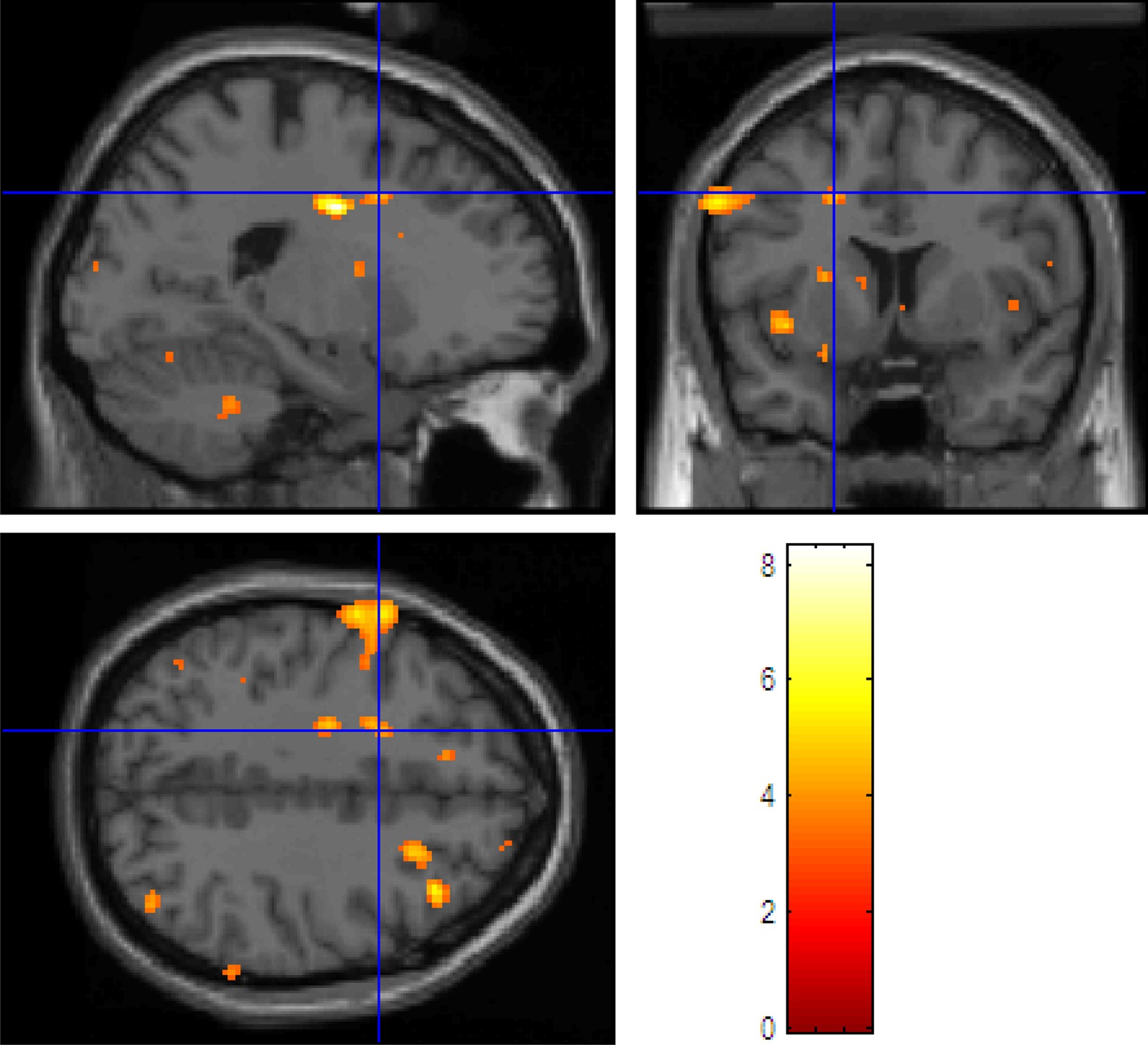
Figure 1. An example fMRI scan showing brain activity.
Second, although time courses are considered continuous, current functional brain imaging devices can only record the brain activity changes discretely. In other words, they measure signal amplitudes at a sample of time points, which is usually evenly spaced (e.g., every 1–2 s). This temporal sampling is relatively sparse, because brain waves for some specific tasks change fast. For example, when studying auditory brainstem, the stimuli are usually brief (e.g., about 100 ms) with several cycles (Roberts and Poeppel, 1996). The change of brain waves is also fast, because the response functions in the brain are highly correlated with the stimuli. The sparse sampling can hardly capture some characteristics of the brain activity.
Third, the hypotheses on how the brain activates are sometimes difficult to formalize. In some cases, the reference function can be used to formulate the hypothesis, but it is not always the case. In many studies there is no such reference function (e.g., decision making, reasoning and emotional processes). In these studies, formulating the hypothetical brain wave has to borrow ideas from many disciplines, including cognitive neuroscience, social psychology, neuropsychology and so on.
The rest of the paper is constructed as follows. In Sections “Dimension Reduction,” “Spatial Classification Problems in fMRI,” and “The Inverse Problem in MEG,” we present three of the issues in brain imaging studies: dimension reduction, spatial classification, and the inverse problem. In each section, we compare different commonly used multivariate and functional methods, and our results show that using FDA can lead to better results in general. The data sets used in this paper are from an fMRI vision study and an MEG somatosensory study.
Dimension Reduction
Functional data is intrinsically infinite-dimensional. Even though they are measured discretely over a finite set of some interval, the dimensionality (i.e., the number of measurements) is high. This introduces the “curse of dimensionality” (Bellman, 1957) and causes problems with data analysis (Aggarwal et al., 2001). High-dimensional data significantly slow down conventional statistical algorithms or even make them practically infeasible. For example, one may wish to classify time courses into different groups. Standard classification methods may suffer from difficulties of handling the entire time courses when the dimension is high. Even if some advanced techniques can be applied to the entire time courses [e.g., support vector machines (SVM) and neural networks (NN)], classification accuracy and computation cost can be significantly improved by using a small subset of “important” measurements or a handful of components that combine in different ways to represent features of the time courses. One reason is that consecutive time points are usually highly correlated, including too much redundancy may increase the noise level and hence mask useful information about the true structure of the data.
In addition, it is usually not necessary to manipulate the entire time course. For the purpose of model interpretation, using a small number of the most informative features may help build a relatively simpler model and reveal the underlying data structure. Hence, one can better explain the relationship between the input and output of the model.
Therefore, dimension reduction (or feature extraction) should be applied to compress the time courses, keeping only relevant information and removing correlations. This procedure will not only speed up but also improve the accuracy of the follow-up analyses. Furthermore, the model may be more interpretable when only a handful of important features are involved.
Let xi(t) be the ith time course, i = 1,2,…,N, where ti ∈ Ti = {ti,1, ti,2,…ti,M}. For notational simplicity, we assume that the Ti’s are the same for all N time courses. Hence, we denote T = {t1, t2,…tM} for all xi(t)’s. Suppose that the reduced data are stored in a matrix, Z ∈ ℝN×K, where each row represents a time course and each column represents a feature in a new coordinate system.
Generally, dimension reduction for functional data can be expressed as:

where zi,k is the (i, k)th element in the reduced data (feature space) Z and fk(t) is some so-called transformation function that transforms xi(t)’s to the new coordinate system.
In the following subsections, we briefly describe three popular dimension reduction approaches that are widely applied to functional neuroimaging studies.
Functional Principal Component Analysis
Functional principal component analysis (FPCA) is an extension of multivariate PCA and was an critical part of FDA in early work. In the context of brain imaging studies, it is especially useful when there is uncertainty as to the duration of a mental state induced by an experimental stimulus, e.g., a decision making process or an emotional reaction. This is because as an explorative technique, FPCA does not make assumptions on the form of brain waves. A few studies have included FPCA. Viviani et al. (2005) used FPCA to single subject to extract the features of hemodynamic response in fMRI studies, and showed that FPCA outperformed multivariate PCA. Long et al. (2005) used FPCA on multiple subjects to estimate the subject-wise spatially varying non-stationary noise covariance kernel.
As with multivariate PCA, FPCA explores the variance–covariance and the correlation structure. It identifies functional principal components that explain the most variability of a set of curves by calculating the eigenfunctions of the empirical covariance operator. FPCA also can be expressed using Eq. 1, in witch the transformation functions, fk(t)’s are orthonormal eigenfunctions. That is,
In the matrix form, Eq. 1 can be expressed as:

where elements in fk and xi are realizations of the kth eigenfunction and the ith observed time course, respectively.
There are several issues when applying FPCA. One is to choose the form of the orthonormal eigenfunctions. Note that any functions can be represented by its orthogonal bases. The choice of the basis decides the shape of the curve. Usually, the bases should be chosen such that the expansion of each curve in terms of these basis functions approximates the curve as closely as possible (Ramsay and Silverman, 2005). That is,
where  Ramsay and Silverman (2005) give a detailed explanation of how to solve for fk(t).
Another issue is to choose the number of eigenfunctions, K. This is an important practical issue without a satisfactory theoretical solution. Presumably, the larger the K, the more flexible the approximation would be, and hence, the closer to the true curve. However, a large K always results in a complex model which introduces difficulties to follow-up analyses. In addition, interpreting a large number of the orthogonal components may be difficult. One wishes every eigenfunction can capture a meaningful feature of the curves so that the components can be interpretable. Simpler models with fewer components are considered more interpretable and hence are more preferable. However, this is not always straightforward in real life. The most commonly used approach to choose K is estimating the number of components based on the estimated explained variance (Di et al., 2009).
Filtering Methods
Another type of approaches that conduct dimension reduction is the so-called filtering methods, which approximate each function by a linear combination of a finite number of basis functions and represent the reduced data by the resulting basis coefficients. Since measurement errors may come along with the data, the observed curves may contain roughness. Filtering methods are put forth to smooth the curve. One can use a K-dimensional basis function to transform xi(t)’s into new features. We write,

where b(t) = [b1(t), b2(t),…,bK(t)]T is a K-dimensional basis function and θi = [θi,1,θi,2,…,θi,K]T is the corresponding coefficient vector of length K. The coefficients θi’s are usually treated as the extracted features. The θi’s can be estimated by using the least squares solution:

where B is defined as the m-by-K matrix containing the values of bk(tj)’s, S = (BTB)−1BT and xi’s are the observed measurements of the ith functional curve at time points T. Hence we have,

where sk, k = 1,2,…,K is the jth row of S and  is the kth estimated coefficient of
  This way a filtering method can also be represented using the same form of Eq. 1. The
  is equivalent to zi,k and sk is equivalent to the realizations of fk at time points T.
One issue with the filtering methods is the selection of basis functions. Commonly used techniques use the Fourier or the wavelet bases to project the signal into the frequency domain or a tiling of the time–frequency plane, respectively. By keeping the first K coefficients as features, each time course is represented by a rough approximation. This is because these coefficients correspond to the low frequencies of the signal, where most signal information is located. Alternatively, one can also use the K largest coefficients instead, because these coefficients preserve the optimal amount of energy present in the original signal (Wu et al., 2000). Criteria for choosing K is similar to choosing K eigenfunctions in FPCA.
A Classification Oriented Method
One alternative to the aforementioned methods is the FAC method proposed by Tian and James (under review). FAC deals with functional dimension reduction problems for classification tasks specifically. This method is highly interpretable and has been demonstrated effective in different classification scenarios. Similarly to FPCA and filtering methods, FAC also follows Eq. 1 and finds a set of fk(t)’s so that the transformed multivariate data Z can be optimally classified. The idea of FAC is expressed as follows:
where scalar Y is the group label, F(t) = [f1(t), f2(t),…,fk(t)]T, ℳF(t) is a pre-selected classification model applied to the lower-dimensional data, e is a loss function resulting from ℳF(t), and γ(F) constrains the model complexity. By adding this constraint, the solution to Eq. 6 can achieve better interpretability. In practice, this constraint can be set to constrain the shape of fj(t)’s. For example, one can let the fj(t) be piecewise constant or piecewise linear. These simple structures are considered more interpretable than structures involving more curvature.
Equation 6 is a difficult non-linear optimization problem and is hard to solve. Tian and James (under review) proposed a stochastic search procedure guided by the evaluation of model complexity. This procedure makes use of the group information and produces simple relationships between the reduced data and the original functional predictor. Therefore, this dimension reduction method is particularly useful when dealing with classification problems (see Spatial Classification Problems in fMRI).
The aforementioned functional methods assume that xi(t)’s are fixed unknown functions. When the noise level is high (e.g., single-trial EEG/MEG), it is difficult to represent the time course properly with a basis expansion having deterministic coefficients. A stochastic representation such as the well-localized wavelet basis (Nason et al., 1999) or the smooth localized Fourier basis (Ombao et al., 2005) may be more preferable.
In many circumstances, the aforementioned dimension reduction methods can efficiently reduce the data dimension and significantly speed up the follow-up analyses. The choice of a dimension reduction method should be guided by the follow-up analyses. For example, if the final goal is extracting orthogonalized lower-dimensional features and there is uncertainty of the mental state, then FPCA may be a better choice. If the goal is further analyzing the data features or feature selections, then filtering methods may be a good option. This is because a filtering method can be performed in the frequency domain. One then selects low-frequency features which contain most signal information. If the final goal is classifying different sets of functions, then FAC may dominate others.
An Example
In this section, we demonstrate the effectiveness of the aforementioned dimension reduction approaches on a classification task in an fMRI study. Since the goal is classification, we expect that the classification oriented FAC method would outperform others in terms of classification accuracy. The idea is to reduce the dimension of the time courses first and then utilize the reduced data as the input of a classification model.
The data set came from a vision study that were conducted in the Imagine Center at the University of Southern California. There are five main subareas in the visual cortex of the brain: the primary visual cortex (striate cortex or V1) and the extrastriate visual cortical areas (V2, V3, V4, and V5). Among them, the primary visual cortex is highly specialized for mapping the spatial information in vision, that is, processing information about static and moving objects. The extrastriate visual cortical areas are used to distinguish fine details of the objects. The main goal for this study is to identify subareas V1 and V3. Presumably, voxel amplitude time courses in the V1 area are different from time courses in the V3 area. Since the boundaries for these two subareas are relatively clear, it is reasonable to utilize these data to evaluate the performance of the aforementioned dimension reduction methods in classification.
The data contain 6924 time courses, where 2058 are from V1 and 4866 are from V3. These time courses are measured at 404 time points. These 404 measurements are averages of three trails. We sample 600 time courses, evenly spaced, from V1. Then we randomly select 500 time courses and put them in the training data, and the rest 100 are placed into the test data. We do the same process to V3 and obtain 500 training time courses and 100 test time courses. Hence, the total training and test data contain 1000 and 200 time courses, respectively. We apply FPCA, filtering methods, and FAC to reduce the dimensionality of the data. For filtering methods, we examine B-Spline bases (Filtering1) and Fourier Bases (Filtering2). For FAC, we examine the piecewise constant version (FAC1) and the piecewise linear version (FAC2). That is, FAC1 constrains fj(t)’s to be piecewise constant and FAC2 constrains fj(t)’s to be piecewise linear. The final classifier is a standard logistic regression. Note that other classifiers can be applied, but we use logistic regression as an example, since the goal is to evaluate dimension reduction methods given a fixed classifier. Tian and James (under review) have compared filtering methods with FAC in the same setting. Here we extend the comparisons to FPCA. We examine when K = 4 and 10. That is, reduce the data to either 4 or 10 dimensions, then apply a logistic regression to the lower-dimensional data. Table 1 shows test misclassification rates on the reduced data. The misclassification rate is defined as the ratio of the number of misclassified test time courses to the total number of test time courses. Note that other criteria can be used to evaluate classification accuracy. Since FAC is a stochastic search based method, we apply it 10 times (with each time 100 iterations) on these data and compute the average test misclassification rate and the standard error (in the parentheses).
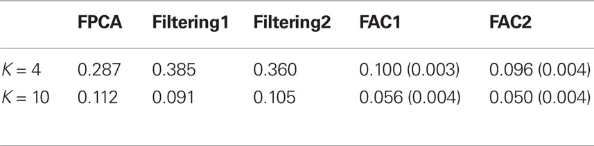
Table 1. Misclassification rates on the reduced data (classifier: logistic regression).
As expected, both versions of FAC outperform other methods in general. In particular, FAC2 provides the best accuracy. Between the other two methods, when K is small FPCA seem to work better than filtering methods, but when K is large filtering methods show slight advantages over FPCA.
One problem with FAC is that it is a stochastic search based method, therefore, the computation cost is more than the other two deterministic methods. We investigate the computation time of these three methods. All methods are implemented in R and run on a 64-bit Dell Precision workstation (CPU 3.20 GHz; RAM 24.0 GB). For FAC1, we examine one run with 100 iterations. We recorded the total CPU time (in seconds) of the R program and list it in Table 2. As we can see, the computation cost for FAC is much higher than that for FPCA and filtering methods, even though its accuracy is high.
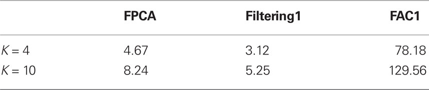
Table 2. Execution time in second.
Again, there is not a universal dimension reduction method. This example only shows the performance of different methods when the final goal is classification. There may be the case that FAC is less preferable when the goal is, say extracting low-frequency features. One need to choose an appropriate method based on the ultimate goal. Also, computation cost is another factor that needs to be considered. One should seek for a balance between accuracy and cost.
Spatial Classification Problems in fMRI
The high spatial resolution of fMRI enables us to obtain more precise and better localized information. Therefore, it is usually used to analyze neural dynamics at different functional regions in the brain. However, it is difficult to identify some small functional subareas for a specific task. One commonly used method is based on theories in neurobiology and cognitive sciences. This is to assume that different functional subareas have different neural dynamic responses (i.e., voxel amplitude functions are different in different subareas) given a specific task. Let us use the visual example again. Based on the visual transmission theories, the visual information is carried out through neural pathways from V1 to V5. The information first reaches the V1 area and then V2 and so on. The neural response functions in these subareas differ in terms of the amplitudes and frequencies. Therefore, by comparing the shape of the neural response functions in different subareas, these visual cortical subareas can be identified. In many fMRI studies so far, this comparison is mostly done by naked eye, which is inefficient and inaccurate. In addition, since, for example, the visual transmission is a non-linear continuous process (Zhang et al., 2006), there is no a clear boundary between two adjacent subareas. The characteristics for voxels near the boundary might be very similar. This results in large within-group variations and, hence, the naked-eye method is unsatisfactory.
Two commonly used techniques for spatial classification are machine learning methods and functional discriminant methods.
Machine Learning Methods
Machine learning methods are applied in two ways. One way is discard temporal orders and treat the time courses as multivariate vectors. Then one can apply classification techniques to these “vectors” directly. To implement, one obtains the data consisting of the neural dynamic response functions and their corresponding class labels. These data should be selected from the region where the class labels are relatively clear, e.g., the center of a subarea. These data are divided into training and test sets. The training data are used to fit the model and select tuning parameters for the model, and the test data are used to examine the performance of the fitted model. Once the model is built, it can be applied to new data where the group labels are unknown.
Since the dimension of the vectors (i.e., the number of measurements in the time courses) can be a few hundred, many standard multivariate classification methods are unsatisfactory. There are some advanced methods designed for high-dimensional data such as SVM (Vapnik, 1998), treed-based methods (Breiman, 2001; Tibshirani and Hastie, 2007), and NN (Hertz et al., 1991). These methods can be applied to handle time courses classification. However, these methods do not consider the functional nature of the time courses and thus have disadvantages. As mentioned earlier, adjacent measurements in a time course are highly correlated. In addition, time courses in functional brain imaging studies contain a lot of noise and important classification information usually lies in small portions of the time courses, e.g., some peak areas. Therefore, it is not necessary to include all measurements in the model.
Another way consists of two parts: dimension reduction and classification. More specifically, first reduce the data dimension and then apply classification techniques to the reduced data. For we have discussed some methods for dimension reduction in Section “Dimension Reduction.” These methods transform the data onto a new feature coordinate system and select a handful of important features in this new coordinate system. Another type of dimension reduction is selecting a subset of relevant measurements from the entire time courses instead of transforming the data. This can be done through a variable selection technique, such as the Lasso (Tibshirani, 1996; Efron et al., 2004), SCAD (Fan and Li, 2001), nearest shrunken centroids (Tibshirani et al., 2002), the Elastic Net (Zou and Hastie, 2005), Dantzig selector (Candes and Tao, 2007), VISA (Radchenko and James, 2008), and FLASH (Radchenko and James, 2010). Then a standard classification technique can be applied to the selected measurements.
Functional Discriminant Methods
Functional discriminant methods have also been studied. These methods consider the functional nature of the time courses. In general, the idea can be viewed as extensions of classical statistics to the functional space. One extension is the generalized linear model in the functional form, i.e., the functional regression model with a scalar response and a functional predictor. Let Y be the categorical response variable. Consider the model,

where yi is the class label for the ith time course and the unknown functional coefficient β(·) measures the dependence of yi on xi. Note that xi(t) is the “true” underlying function for the ith time course and it is unobserved. The measurement xi,j is the perturbed value of xi(t) at time tj and the perturbation is ei.
To solve Eq. 7, many methods were proposed. Some examples are the generalized singular value decomposition (SVD) method (Alter et al., 2000), the linear discriminant method for sparse functional data (James and Hastie, 2001), the parametric method with the generalized linear model involved (James, 2002; Müller, 2005; Müller and Stadtmüller, 2005), non-parametric methods (Hall et al., 2001; Ferraty and Vieu, 2003), the smoothing penalization method (Ramsay and Silverman, 2005), the factorial method of testing various sets of curves (Ferraty et al., 2007), and the robust method with estimation of the data depth (Cuevas et al., 2007).
Many of the aforementioned methods involve a dimension reduction step as well. For example, Alter et al. (2000), Hall et al. (2001), and Müller and Stadtmüller (2005); Müller (2005) used the Karhunen–Loève decomposition to transform the covariance function to a diagonalized space. James (2002); James and Hastie (2001) used filtering methods to approximate xi(t)’s and β(t), i.e., using coefficients of basis functions instead of the original measurements. We describe three methods below.
James (2002) used natural cubic spline (NCS) bases to expand xi,j’s and approximate the β(t).


where φ is a K-dimensional NCS basis, zi is its corresponding coefficient vector, and ψ is a L-dimensional NCS basis. Equation 8 expands the (i,j)th measurement by its basis functions. Equation 9 approximates β(t) by its basis. The coefficient vector c can be estimated using the maximum likelihood method.
Müller (2005) used the Karhunen–Loève decomposition to decompose xi(t)’s to a diagonalized space. In this case, Eq. 3 is used to approximate xi(t)’s, b(t) contains the first K eigenfunctions of xi(t)’s and θi,k’s are all uncorrelated, i.e., the variance–covariance matrix is diagonal. Then Eq. 7 can be written as:
Let ηk = ∫β(t)bk(t) dt. Then ηk’s can be estimated by regressing yi on θi,1,…,θi,K
Hence, this method is a two-step approach. The first step is dimension reduction, then the second step is classification.
Ramsay and Silverman (2005) approximated xi(t) and β(t) using Eqs 3 and 9, respectively, with a large number of bases for xi(t)’s. We write,
X(t) = θb(t)
where the coefficient matrix θ is N-by-K. Then Eq. 7 becomes

where X(t) = [x1(t),…,xN(t)]T, Ω = ∫ b(t)c(t)Tdt is a K-by-L matrix. Then β(t) can be estimated by minimizing a penalized residual sum of squares:
where λ is some smoothing parameter and L is a linear differential operator.
As mentioned earlier, one potential limitation of the aforementioned functional methods is that when the noise level in the observed time courses is high. These data cannot be adequately represented by FDA when the coefficients are assumed fixed but unknown. Stochastic coefficient methods (Nason et al., 1999; Ombao et al., 2005) may provide better solutions. For example, Ho et al. (2008) utilized the Ombao et al. (2005)’s method to capture the transient features of brain signals in the frequency domain, then used relevant time–frequency features to distinguish between groups.
An Example
In this section, we examine the performance of four methods on a spatial classification task. The four methods include three machine learning methods and one functional discriminant method. First, we apply SVM directly to the entire time courses treating them as multivariate vectors. Second, we apply a filtering method to reduce the data dimension, then apply SVM. The basis used in the filtering method is a 10-dimensional NCS. Third, we apply the Lasso (Tibshirani, 1996) to select 10 measurements from the time courses and then apply SVM. Finally, we apply the smoothing penalization method (Ramsay and Silverman, 2005) to the time courses. This method is implemented in the R library fda.
We use the same fMRI vision data as in Section “An Example” and the goal is to identify subareas V1 and V3. For each subarea 600 time courses are selected. Misclassification rates are estimated by a 10-fold cross-validation. That is, the data are divided by 10 parts equally. Each part contains 60 time courses from V1 and 60 time courses from V2. First, part number one is used as the test data and the rest nine parts are used as the training data. Then part number two is used as the test data and the rest nine parts as the training data. This procedure is conducted 10 times and all parts are used as the test data once. The misclassification rate is estimated by averaging the 10 test errors.
The results are listed in Table 3, in which full-SVM represents applying SVM directly to the entire time courses, filter-SVM represents using filtering methods to reduce the data dimension and then applying SVM to the reduced data, Lasso-SVM represents using the Lasso to select measurements first and then applying SVM, and Smoothing represents applying the smoothing penalization method. As we can see, filter-SVM produces the best result, while full-SVM provides the worst result. Comparing Table 3 to Table 1, FAC2 plus logistic regression classifier outperforms the four methods listed in this section. This indicates that a good dimension reduction method can improve classification results. Using filtering methods to reduce the data dimension may lose some useful information for classification. Therefore, even though SVM is thought to be more advanced than logistic regression, it may not be good enough to compensate for the loss of information by filtering methods. One may expect that the classification accuracy will improve when SVM is applied after FAC.
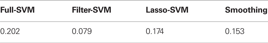
Table 3. Estimated misclassification rates by a 10-fold cross-validation.
The Inverse Problem in MEG
Magneto-encephalography is a non-invasive powerful technique that can track the magnetic field accompanying synchronous neuronal activities with temporal resolution easily reaching millisecond level. Therefore, it is able to capture the rapid change in cortical activity. With recent development of whole-head biomagnetometer systems that provide high spatial resolution in magnetic field coverage, MEG possesses unique capability to localize the detected neuronal activities and follow its changes millisecond by millisecond when suitable source modeling techniques are utilized. Thus it is attractive in cognitive studies of normal subjects and in neurological or neurosurgical evaluation of patients with brain diseases. In MEG studies, evoked responses are measured over time by a set of sensors outside the head of a patient. One of the issues is reconstructing and localizing the signal sources of evoked events of interest in the brain based on the measured MEG time courses. This is the so-called “inverse problem.”
For example, in a somatosensory experiment, data were recorded by an MEG device with 247 sensors (channels). Each sensor records 228 measurements during one trail. One then averages all three trails. Figure 2 shows the time courses from the 247 channels (left panel) and their corresponding isofield magnetic maps (right panel), respectively. Stimuli were presented at time points 85 and 99. As we can see from the left panel of Figure 2, the evoked activity time courses achieve the peaks at 85 and 99. We expect that the reconstructed source time courses can reflect the peak activities, because the correlation between stimuli and brain responses is high. That is, the reconstructed curves should have significant activations in the somatosensory area at the corresponding time points 85 and 99.
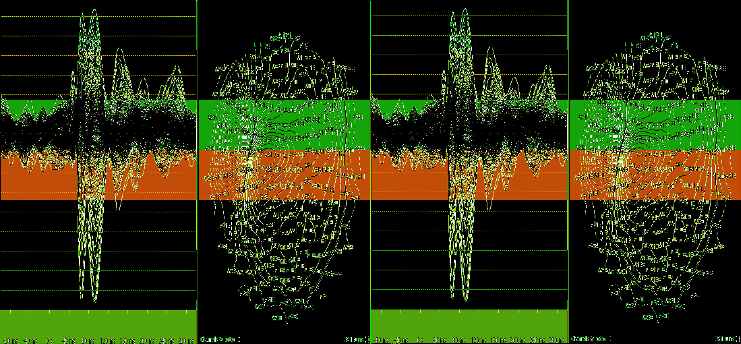
Figure 2. Left panel: measured time series from all sensors; right panel: isofield magnetic map.
There are two main types of methodologies to formulate and solve the inverse problem: the parametric methods and the non-parametric methods. The parametric methods are also referred to as equivalent current dipole methods or dipole fitting methods. Examples of these methods include the multiple signal classification (MUSIC) method (Mosher et al., 1992), the linearly constrained minimum variance (LCMV) beamformer method (VanVeen et al., 1997) and so on. These methods evaluate the best positions and orientations of a dipole or dipoles and are more apt to be physics based methods.
The non-parametric methods are also referred to as the imaging methods. These methods are more apt to be statistical based methods and will be discussed in the following subsections. The non-parametric methods are based on the assumption that the primary signal sources can be represented as linear combinations of neuron activities (Barlow, 1994). Therefore, the inverse problem can be formulated through a non-parametric linear model,

where y(t) = [y1(t), y2(t),…,yN(t)]T is a set of MEG time courses recorded by N sensors and β(t) = [β1(t), β2(t),…, βp(t)]T is a set of source time courses at the cortical area, where p is the number of potential sources. The forward operator X is an N-by-p matrix representing the propagation of the magnetic field in the cortical surface. The columns of X are called the “forward fields” and the rows of X are called the “lead fields.” Each forward field describes the effect of one given source to the observed measurements across sensors, and each lead field describes the combined effects of all sources to a given sensor (Ermer et al., 2001). X can be computed by a simple spherical head model (Mosher et al., 1999), and hence, it can be treated as known. The vector e(t) = [e1(t), e2(t),…, eN(t) T is the noise time series during the experiment. Model (see A Basis Expansion Method) is a non-parametric model in which the parameters, βj(t)’s (j = 1,…,p), are non-parametric smooth functions. The problem is to estimate βj(t)’s.
Based on brain anatomical theories, each neuron in the cortical area can be a potential source, so p can be the number of neurons. In practice, it is infeasible to reach the neuron level. Instead, the cortical area is divided into small regions in the millimeter scale. The head model considers each region as a source, and p is the number of these small regions in the cortical area. This number can be a tens of thousands. However, present MEG devices have at most a few hundred sensors. For example, in the somatosensory example showed at the beginning of Section “The Inverse Problem in MEG,” there are 247 sensors and hence only 247 measured time courses. Therefore, p ≫ N and this inverse problem is highly ill-posed.
Several methods have been proposed to tackle this problem. We describe three types of methods here: regularization methods, spatio-temporal methods, and functional methods.
Regularization Methods
In the matrix form, we write,

where Y is an N-by-s matrix representing the N measured EEG/MEG time courses over s time points. Elements in Y are measurements of the N functions over s time points with perturbations. X is still the N-by-p forward operator, β is a p-by-s matrix representing realizations for p source time courses at s time points, and E is an N-by-s noise matrix.
Since p ≫ N, Eq. 14 cannot be solved directly. Regularization is a commonly used technique to solve Eq. 14, and the solution can be expressed as:

where ||·||F is known as the Frobenius norm of a matrix, L is a penalty function and λ ≤ 0 is a fixed penalty parameter that controls the degree of regularization. Some well-known regularization methods impose the Tikhonov regularization (L2-penalty) on β, i.e., L(β) = ||β||2, or some modifications of L2. These methods include the minimum norm estimate (MNE) (Hämäläinen and Ilmoniemi, 1984; Dale and Sereno, 1993), the weighted minimum norm estimate (WMNE) (Iwaki and Ueno, 1998), the focal underdetermined system solver (FOCUSS) (Gorodnitsky and Rao, 1997) and the low resolution electrical tomography (LORETA) (Pascual-Marqui et al., 1994). However, applying L2-norm to the entire β space makes the solution too diffuse. According to brain anatomical theories, the source time courses should be relatively “sparse” in the spatial domain for a given task. That is, only some compact subareas are active at the same time, while a large area of the brain should stay inactive. Time courses in active areas should have significantly larger amplitudes than that in inactive areas. Due to the nature of the L2-penalty, the results from L2-penalty based methods are too diffuse in the spatial domain and are unsatisfactory in terms of localizing sparse active areas.
One alternative to the L2-penalty is the minimum current estimate (MCE) and its modifications (Uutela et al., 1999; Lin et al., 2006), which impose the L1-penalty, i.e., L(β) = |β|. MCE can produce better solutions in terms of identifying sparse active areas due to the nature of the L1-penalty. However, MCE introduces substantially discontinuities to the source time courses. Hence, the “spiky-looking” time courses will be observed. As described, the advantages and disadvantages of L2 and L1 methods are complementary.
The aforementioned L2 and L1 based regularization methods were originally designed for parametric regression problems and are hardly applied to the non-parametric problems where βj(t)’s are smooth functions. Functional methods that take into account the functional nature of the data are in strong demand. These methods involving include the L1L2-norm inverse solver (Ou et al., 2009) and the functional expansion regularization (FUNER) approach (Tian and Li, under review). We briefly present these two methods in the following subsections.
A Spatio-Temporal Method
The L1L2-norm method assumes the signal times courses the MEG time courses can be represented by their lower-dimensional temporal basis functions. Then it attempts to estimate their temporal coefficients instead of estimating the entire time courses. Since y(t) is evoked by β(t), it is natural to assume that β(t) and y(t) share the same temporal bases. Suppose that y(t) and β(t) can be approximated by the same K-dimensional temporal basis. That is, we let  and
and  where ψk(t) is the kth basis function,
  is the kth coefficient for the ith MEG time course and
  is the kth coefficient for the jth source time course. Then Equation (14) can be simplified by:

where 
 and
and  are all N-by-K coefficient matrices for their basis functions. A smooth temporal domain and a sparse spatial domain can be achieved by imposing an L2-penalty to the temporal domain and an L1-penalty to the spatial domain, i.e.,
Then the minimization problem can be treated as a second-order cone programming problem and hence solved.
A Basis Expansion Method
The FUNER method also uses basis approximation, and imposes L2-penalty and L1-penalty to the source time courses. But instead of applying constraints to the coefficient matrices, FUNER projects the source spatio-temporal information onto one hyperplane, and imposes an L2-penalty to the temporal information and an L1-penalty to the spatial information on this hyperplane simultaneously. Assuming b(t) is a K-dimensional temporal basis for βj(t)’s, FUNER modifies Model as follows:

where  and
and  containing coefficient vectors for b(t). In matrix notation, Eq. 18 can be expressed as:

where  is an Ns-vector of the new expanded response variable,
  is an Ns-vector of the new white noise variable, and
where each block element,  (e.g.,
  ), is a K-vector. This way, the original inverse problem has been modified as solving a high-dimensional linear regression problem (Eq. 19). Each block in X* contains all spatial and temporal information for one source time course. One can treat each block as a group and apply some group shrinkage techniques, such as the group Lasso (Yuan and Lin, 2006), to Eq. 19 to shrink coefficients within an inactive group all toward zero.
The two functional methods described in Sections “A Spatio-Temporal Method” and “A Basis Expansion Method” have shown advantages over some commonly used multivariate methods in terms of reconstruct signal time courses (TOu et al., 2009; ian and Li, under review).
An Example
In this section, we provide comparisons of the FUNER method and two regularization methods: MNE and MCE on an real-world MEG data. The data were from the somatosensory study described in the beginning of Section “The Inverse Problem in MEG.” The data were obtained from the Center for Clinical Neurosciences at the University of Texas Health Science Center. For the FUNER method, we apply two bases: NCS with K = 7 bases functions and the first K = 7 bases from SVD of Y.
We are interested in the activation map at time points 85 and 99. Figure 3 shows side views of the 3-dimensional brain maps at time point 85 by the three methods. Among these four figures, FUNER with SVD bases is the best because it correctly identifies the somatosensory area (located at the left postcentral gyrus) and the active area is very focal. MCE is the second best because it also correctly identifies part of the somatosensory area but the active area is not large enough. The active area from FUNER with a NCS basis is too focal, so this method is relatively less satisfactory comparing to FUNER (SVD) and MCE. MNE is the worse method among the four methods, because the active areas from MNE are too broad. It picks out the somatosensory area but also incorrectly picks out some inactive areas.
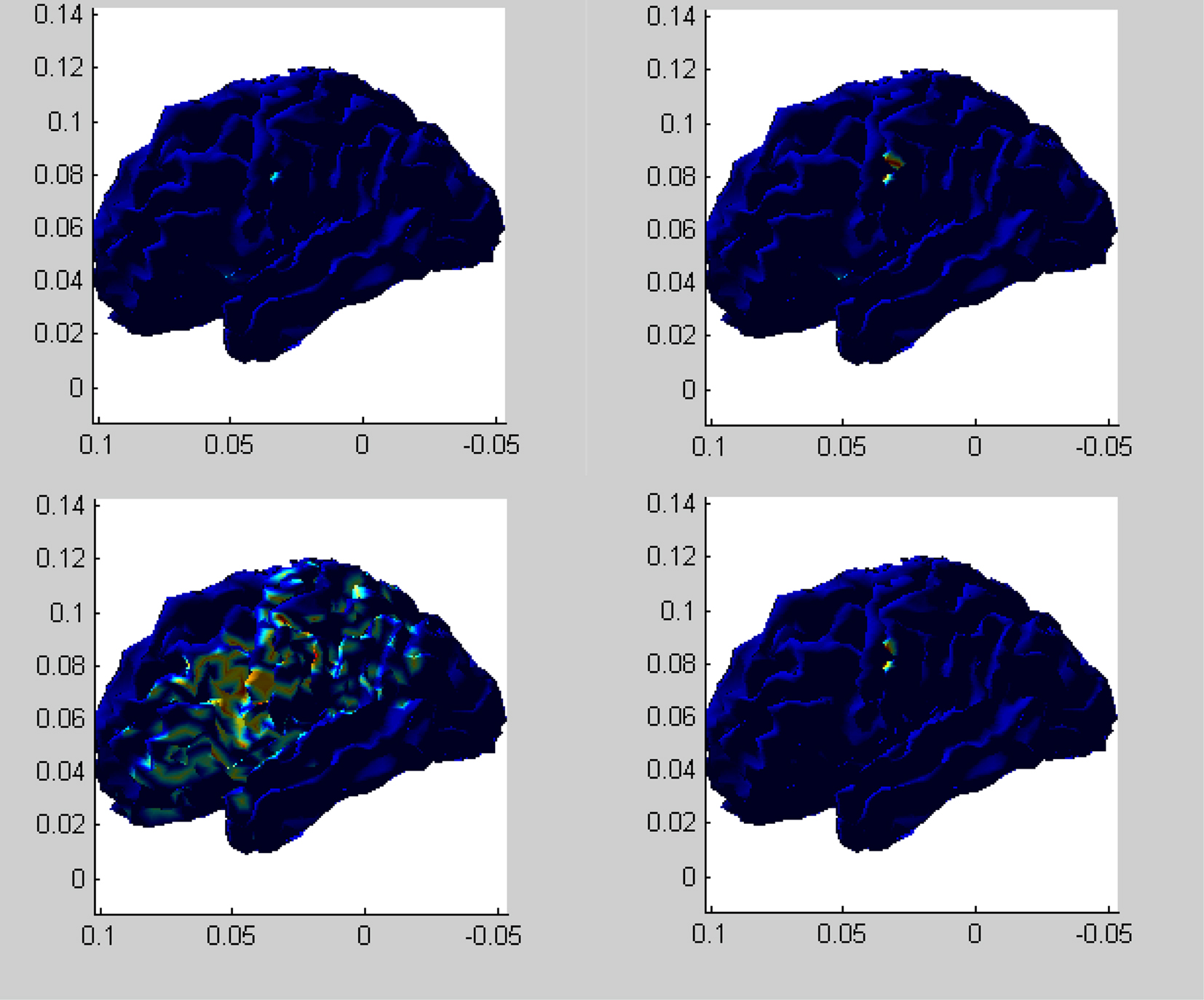
Figure 3. Reconstructed source maps at time point 85 (the side view). Upper left panel: FUNER (NCS); upper right panel: FUNER (SVD); lower left panel: MNE; lower right panel: MCE.
We also examine the computation cost in this example. All methods are implemented in R and the computation time is recorded in Table 4. As we can see, the execution time for FUNER is much higher than MNE and MCE. This is because FUNER expands the data to a higher-dimensional space and makes the already large data even larger.
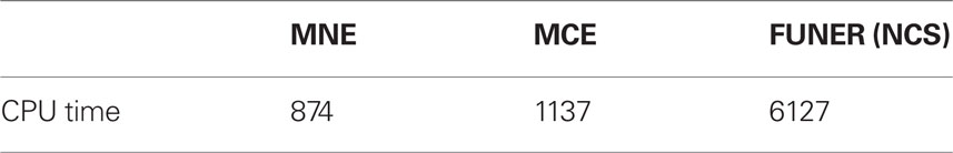
Table 4. Eexecution time in second.
This example shows that some functional methods can provide better results than multivariate methods in terms of accuracy, but the computation cost may be high.
Conclusions and Discussions
Functional data analysis applied on functional brain imaging studies has become more and more prevalent nowadays. We have briefly discussed three issues, dimension reduction, spatial classification and the inverse problem, that occur in functional brain imaging studies. They are problems with strong demands on FDA techniques.
There are three major challenges in applying FDA to functional brain imaging studies. First and foremost, the computational cost is a big issue due to the large volume of brain imaging data. In particular, when some method requires a stochastic search or an expansion of the data by their basis functions, the issue will be aggravated (see Tables 2 and 4). Although most of the brain imaging problems focus on accuracy rather than real-time processing performance, computation efficiency is still an important factor to consider. Second, most FDA techniques that deal with brain imaging data assume that the error term is independent and identically distributed white noise. However, the noise is rarely normally distributed. For example, in fMRI studies, sources of noise include low-frequency drift due to machine imperfections, oscillatory noise due to respiration and cardiac pulsation, residual movement artifacts and so on. Further investigation that considers different noise patterns and dependencies is needed. Third, since brain images are naturally 3-dimensional, the observed times courses are not independent from each other. Correlations are higher between time courses in a neighboring region than that between time courses that are far away. Therefore, spatial properties should be taken into considerations as well.
There are many other issues and problems also desire FDA, such as the EEG/MEG sensor evaluation and fMRI pattern classification. The former needs to identify important sensors based on the measured time courses from multiple subjects (Coskun et al., 2009). One of the most commonly used techniques is the T-test, which is far from satisfactory. More sophisticated FDA techniques should be investigated and applied. The latter needs to identify brain state associated with a stimulus. A large amount of research devoted to machine learning methods (see, for example, Martinez-Ramon et al., 2006; Pereira et al., 2009; Tian et al., 2010). However, less research has been conducted on FDA techniques even though they are just as useful as machine learning techniques. FDA methods should also be investigated for these problems.
Conflict of Interest Statement
The author declares that the research was conducted in the absence of any commercial or financial relationships that could be construed as a potential conflict of interest.
References
Aggarwal, C. C., Hinneburg, A., and Keim, D. A. (2001). “On the surprising behavior of distance metrics in high dimensional space,” in Lecture Notes in Computer Science, eds J. Van den Bussche and V. Vianu (London: Springer-Verlag), 420–434.
Alter, O., Brown, P., and Bostein, D. (2000). Singular value decomposition for genome-wide expression data processing and modeling. Proc. Natl. Acad. Sci. U.S.A. 97, 10101–10106.
Barlow, H. B. (1994). “What is the computational goal of the neocortex?,” in Large-Scale Neuronal Theories of the Brain, eds C. Koch and J. L. Davis (Cambridge, MA: MIT press), 1–22.
Candes, E., and Tao, T. (2007). The Dantzig selector: statistical estimation when p is much larger than n (with discussion). Ann. Stat. 35, 2313–2351.
Coskun, M. A., Varghese, L., Reddoch, S., Castillo, E. M., Pearson, D. A., Loveland, K. A., Papanicolaou, A. C., and Sheth, B. R. (2009). Increased response variability in autistic brains? Neuroreport 20, 1543–1548.
Cuevas, A., Febrero, M., and Fraiman, R. (2007). Robust estimation and classification for functional data via projection-based depth notions. Comput. Stat. 22, 481–496.
Dale, A. M., and Sereno, M. I. (1993). Improved localization of cortical activity by combining EEG and MEG with MRI cortical surface reconstruction: a linear approach. J. Cogn. Neurosci. 5, 162–176.
Di, C.-Z., Crainiceanu, C. M., Caffo, B. S., and Punjabi, N. M. (2009). Multilevel functional principal component analysis. Ann. Appl. Stat. 3, 458–488.
Efron, B., Hastie, T., Johnstone, I., and Tibshirani, R. (2004). Least angle regression. Ann. Stat. 32, 407–451.
Ermer, J. J., Mosher, J. C., Baillet, S., and Leahy, R. M. (2001). Rapidly recomputable EEG forward models for realistic head shapes. Phys. Med. Biol. 46, 1265–1281.
Fan, J., and Li, R. (2001). Variable selection via nonconcave penalized likelihood and its oracle properties. J. Am. Stat. Assoc. 96, 1348–1360.
Ferraty, F., and Vieu, P. (2003). Curves discrimination: a nonparametric functional approach. Comput. Stat. Data Anal. 44, 161–173.
Ferraty, F., Vieu, P., and Viguier-Pla, S. (2007). Factor based comparison of groups of curves. Comput. Stat. Data Anal. 51, 4903–4910.
Gorodnitsky, I. F., and Rao, B. D. (1997). Sparse signal reconstruction from limited data using focuss: a re-weighted minimum norm algorithm. IEEE Trans. Signal Process. 45, 600–616.
Hall, P., Poskitt, D. S., and Presnell, B. (2001). A functional data-analytic approach to signal discrimination. Technometrics 43, 1–9.
Hämäläinen, M., and Ilmoniemi, R. J. (1984). Interpreting Measured Magnetic Fields of the Brain: Estimates of Current Distribution. Technical Report, TKK-F-A599. Espoo: Helsinki University of Technology.
Hertz, J., Krogh, A., and Palmer, R. G. (1991). Introduction to the Theory of Neural Computation. Reading, MA: Addison-Wesley.
Ho, M.-H. R., Ombao, H., Edgar, J. C., Caive, J. M., and Miller, G. A. (2008). Time–frequency discriminant analysis of MEG signals. Neuroimage 40, 174–186.
Iwaki, S., and Ueno, S. (1998). Weighted minimum-norm source estimation of magnetoencephalography utilizing the temporal information of the measured data. J. Appl. Phys. 83, 6441–6443.
James, G. (2002). Generalized linear models with functional predictors. J. R. Stat. Soc. Series B 64, 411–432.
James, G., and Hastie, T. (2001). Functional linear discriminant analysis for irregularly sampled curves. J. R. Stat. Soc. Series B 63, 533–550.
Lin, F.-H., Belliveau, J. W., Dale, A. M., and Hämäläinen, M. S. (2006). Distributed current estimates using cortical orientation constraints. Hum. Brain Mapp. 27, 1–13.
Long, C., Brown, E., Triantafyllou, C., Aharon, I., Wald, L., and Solo, V. (2005). Nonstationary noise estimation in functional MRI. Neuroimage 28, 890–903.
Martinez-Ramon, M., Koltchinskii, V., Heilman, G., and Posse, S. (2006). FMRI pattern classification using neuroanatomically constrained boosting. Neuroimage 31, 1129–1141.
Mosher, J., Lewis, P., and Leahy, R. (1992). Multiple dipole modeling and localization from spatio-temporal MEG data. IEEE Trans. Biomed. Eng. 39, 541–557.
Mosher, J. C., Leahy, R. M., and Lewis, P. S. (1999). EEG and MEG: forward solutions for inverse methods. IEEE Trans. Biomed. Eng. 46, 245–259.
Müller, H. G. (2005). Functional modelling and classification of longitudinal data. Scand. J. Stat. 32, 223–240.
Müller, H. G., and Stadtmüller, U. (2005). Generalized functional linear models. Ann. Stat. 33, 774–805.
Nason, G. P., von Sachs, R., and Kroisandt, G. (1999). Wavelet processes and adaptive estimation of the evolutionary wavelet spectrum. J. R. Stat. Soc. Series B 62, 271–292.
Ombao, H., von Sachs, R., and Guo, W. (2005). SLEX analysis of multivariate nonstationary time series. J. Am. Stat. Assoc. 100, 519–531.
Ou, W., Hämäläinen, M., and Golland, P. (2009). A distributed spatio-temporal EEG/MEG inverse solver. Neuroimage 44, 932–946.
Pascual-Marqui, R. D., Michel, C. M., and Lehmann, D. (1994). Low resolution electromagnetic tomography: a new method for localizing electrical activity in the brain. Int. J. Psychophysiol. 18, 49–65.
Pereira, F., Mitchell, T., and Botvinick, M. (2009). Machine learning classifiers and FMRI: a tutorial overview. Neuroimage 45, 199–209.
Radchenko, P., and James, G. (2008). Variable inclusion and shrinkage algorithms. J. Am. Stat. Assoc. 103, 1304–1315.
Ramsay, J. O., and Dalzell, C. (1991). Some tools for functional data analysis (with discussion). J. R. Stat. Soc. Series B 53, 539–572.
Roberts, T. P., and Poeppel, D. (1996). Latency of auditory evoked m100 as a function of tone frequency. Neuroreport 7, 1138–1140.
Tian, T. S., James, G. M., and Wilcox, R. R. (2010). A multivariate stochastic search method for dimensionality reduction in classification. Ann. Appl. Stat. 4, 339–364.
Tibshirani, R. (1996). Regression shrinkage and selection via the lasso. J. R. Stat. Soc. Series B 58, 267–288.
Tibshirani, R., and Hastie, T. (2007). Margin trees for high-dimensional classification. J. Mach. Learn. Res. 8, 637–652.
Tibshirani, R., Hastie, T., Narasimhan, B., and Chu, G. (2002). Diagnosis of multiple cancer types by shrunken centroids of gene expression. Proc. Natl. Acad. Sci. U.S.A. 99, 6567–6572.
Uutela, K., Hämäläinen, M., and Somersalo, E. (1999). Visualization of magnetoencephalographic data using minimum current estimates. Neuroimage 10, 173–180.
VanVeen, B., van Drongelen, W., Yuchtman, M., and Suzuki, A. (1997). Localization of brain electrical activity via linearly constrained minimum variance spatial filtering. IEEE Trans. Biomed. Eng. 44, 867–880.
Viviani, R., Grön, G., and Spitzer, M. (2005). Functional principal component analysis of FMRI data. Hum. Brain Mapp. 24, 109–129.
Wu, Y.-L., Agrawal, D., and Abbadi, A. E. (2000). “A comparison of DFT and DWT based similarity search in time-series databases,” in Proceedings of the 9th International Conference on Information and Knowledge Management, McLean, VA, 488–495.
Yuan, M., and Lin, Y. (2006). Model selection and estimation in regression with grouped variables. J. R. Stat. Soc. Series B 68, 49–67.
Zhang, Y., Pham, B., and Eckstein, M. (2006). The effect of nonlinear human visual system components on performance of a channelized hotelling observer in structured backgrounds. IEEE Trans. Med. Imaging 25, 1348–1362.
Keywords: functional data analysis, brain imaging, dimension reduction, spatial classification, inverse problem
Citation: Tian TS (2010) Functional data analysis in brain imaging studies. Front. Psychology 1:35. doi: 10.3389/fpsyg.2010.00035
Received: 18 February 2010;
Paper pending published: 21 March 2010;
Accepted: 03 July 2010;
Published online: 08 October 2010
Edited by:
Moon-Ho R. Ho, Nanyang Technological University, SingaporeReviewed by:
Hernando Ombao, Brown University, USAJiguo Cao, Simon Fraser University, Canada
Copyright: © 2010 Tian. This is an open-access article subject to an exclusive license agreement between the authors and the Frontiers Research Foundation, which permits unrestricted use, distribution, and reproduction in any medium, provided the original authors and source are credited.
*Correspondence: Tian Siva Tian, 126 Heyne Building, University of Houston, Houston, TX 77204, USA. e-mail: ttian@uh.edu