The Joint Distribution Criterion and the Distance Tests for Selective Probabilistic Causality

A general definition and a criterion (a necessary and sufficient condition) are formulated for an arbitrary set of external factors to selectively influence a corresponding set of random entities (generalized random variables, with values in arbitrary observation spaces), jointly distributed at every treatment (a set of factor values containing precisely one value of each factor). The random entities are selectively influenced by the corresponding factors if and only if the following condition, called the joint distribution criterion, is satisfied: there is a jointly distributed set of random entities, one entity for every value of every factor, such that every subset of this set that corresponds to a treatment is distributed as the original variables at this treatment. The distance tests (necessary conditions) for selective influence previously formulated for two random variables in a two-by-two factorial design (Kujala and Dzhafarov, 2008, J. Math. Psychol. 52, 128–144) are extended to arbitrary sets of factors and random variables. The generalization turns out to be the simplest possible one: the distance tests should be applied to all two-by-two designs extractable from a given set of factors.

A system’s behavior, be the system biological, social, or technological, can be thought of as a network of stochastically interdependent random entities. The external world provides inputs (influences, interventions, conditions) presumably affecting some of the components of the network and not affecting the others. The question arises therefore as to how, based on the joint distributions of all these random entities, to distinguish the components affected and not affected by each of these external inputs.

The notion of selective influence under stochastic interdependence was introduced and systematically analyzed in the behavioral context by Townsend (1984), although implicitly it had been used before (Lazarsfeld, 1965; Bloxom, 1972; Schweickert, 1982). Townsend’s approach to selective influence (further developed in Townsend and Thomas, 1994, and mathematically characterized in Dzhafarov, 1999) is, however, very different from the present one. In fact, in all non-trivial cases they are incompatible. Our approach gradually developed starting with Dzhafarov (2001), based on Dzhafarov’s earlier work on response time analysis (see Dzhafarov, 1997, for an overview). In Dzhafarov (2003) the definition of selective influence adopted in the present paper was given for finite systems of random entities. This notion was put on a more solid probabilistic foundation in Dzhafarov and Gluhovsky (2006), and further developed in Kujala and Dzhafarov (2008). In the latter work, for the first time, workable tests for selective influence were formulated.

The present paper continues this line of research on a higher level of mathematical rigor and arguably the highest possible level of generality. The abstract nature of the mathematical theory makes it rather difficult reading, with notation which, though carefully chosen, may appear complicated. As a partial remedy, we precede the formal development in Sections 2–5 by Section 1 in which we provide a more intuitive account of some of the basic notions and results. We do this on simple examples involving just two random variables influenced by two factors.

1. Intuitive Introduction

1.1. What is Selective Influence?

Consider a simple double-detection experiment: there are two stimuli each of which may possess or lack a certain feature (signal property), and an observer has to respond Yes (signal present) or No (signal absent) to each of the two stimuli. For instance, the stimuli may be two spatially separated line segments in a frontal plane each of which may be either vertical (signal absent) or tilted by a fixed small angle (signal present); the observer says Yes − Yes if both lines appear to be tilted, Yes − No if the left line appears tilted and the right one not, etc. These responses are random variables: A (response to the left stimulus) and B (response to the right one), each with two possible values {Yes, No} occurring with some probabilities. They are jointly distributed, in the sense that by the virtue of co-occurring in the same trial the values of A and B are naturally paired, enabling one to meaningfully pose questions like “What is the joint probability of A = Yes and B = No?”. The joint distribution of A and B may change depending on the values of the following external factors: α = Tilt of the left line, with two possible values, {absent, present}, and β = Tilt of the right line, with the same two values. The combination of factor values chosen, one for each of the factors, is traditionally referred to as a treatment. With this terminology and notation, the population-level (idealized) results of the experiment in question can be presented in the form of four matrices:

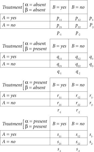
The letters p, q, r, s here represent theoretical probabilities, with the usual meaning of the subscripts: p_1· = p₁₁ + p₁₂, p_2· = p₂₁ + p₂₂, p_1· + p_2· = 1, etc. It is natural to surmise that, unless the observer does not look at the stimuli at all, the random variable A should depend on (be influenced by) the value of α, and B should be influenced by the value of β. It is not obvious, however, whether factor α only (or selectively) influences random variable A, without affecting B, and whether factor β only (selectively) influences random variable B, without affecting A:

as opposed to the possibilities

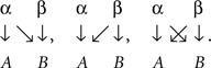
Thus, we will have one of the latter scenarios if the “present” value of α visually masks or enhances the salience of the “present” value of β, or if the values of β somehow affect the level of attention the observer pays to the factor α.

We denote the case when (α, β) selectively influence (A, B), respectively, by

What does this mean? The meaning of the relation is only obvious if A and B are stochastically independent for all four treatments, i.e., if p_ij = p_i· p_·j, q_ij = q_i·q_·j, etc., where i, j ∈{1, 2}. In this case all one has to establish to prove (A, B) ↫ (α, β) is that the marginal distribution of A is not affected by changes in β and the marginal distribution of B is not affected by changes in α.

To look at this in detail, let the pair of our random variables (A, B) at the four treatments be denoted (A, B)₁₁, (A, B)₁₂, (A, B)₂₁, and (A, B)₂₂, where 1, 2 denote “absent” and “present,” respectively. If A and B are independent at all four treatments, then the selectiveness (A, B) ↫ (α, β) simply means that the marginal distribution of A does not depend on β (i.e., p_1· = q_1· and r_1· = s_1·) and the marginal distribution of B does not depend on α (i.e., p_·1 = q_·1 and r_·1 = s_·1). The problem arises when A and B are not independent for at least one of the treatments: how should one determine then if (A, B) ↫ (α, β)? This is the problem addressed in this paper, only we do not confine the consideration to the case of two factors and two random variables. Rather we generalize the problem to an arbitrary set of external factors and an arbitrary (but one-to-one corresponding to the set of factors) set of random entities.¹

For a finite set of random variables the definition of selective influence was given in Dzhafarov (2003) and then refined in Dzhafarov and Gluhovsky (2006) and Kujala and Dzhafarov (2008). Applying it to our example, (A, B) is selectively influenced by (α, β) if and only if one can find functions f and g and a random entity C whose distribution does not depend on α, β, such that

where ∼ stands for “is distributed as”.² That is, denoting f(α = 1, C) by f₁(C), g(β = 2, C) by g₂(C), etc.,

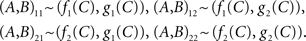
As an example, let C be a random vector (C₀, C_I, C₂) with stochastically independent components having the following interpretation: C₀ is a random entity representing the general level of visual attention, while C₁ and C₂ are stimulus-specific sources of randomness (which, with no loss of generality, can be taken to be uniformly distributed between 0 and 1). Let

where h₁, h₂ are some measurable functions from the set of possible values of C into interval [0, 1]. One can see that A and B are generally stochastically interdependent by virtue of depending on one and the same random entity, C₀, but that A does not depend on β, in the sense that for any given values of the other arguments, C₀ = c₀, C₁ = c₁, C₂ = c₂, and α = 1 or 2, the value of A does not change as a function of β; and B does not depend on α in the analogous sense.

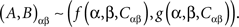
The definition of selective influence can also be looked at in a simpler and more fundamental way. The fact that for any given treatment A and B are stochastically related (i.e., paired, whether independent or interdependent) means in Kolmogorov’s probability theory that A and B are measurable functions of one and the same random entity. It is always true therefore that

The random entities C₁₁, C₁₂, C₂₁, C₂₂, can always be replaced with a single C, e.g., by putting C = (C₁₁, C₁₂, C₂₁, C₂₂) and redefining the functions f, g accordingly:

Comparing this universal representation with (1) we see that the assumption of selective influence is that β in f and α in g are dummy arguments.

1.2. Main Properties of Selective Influence

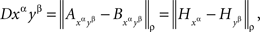
There are three main properties of the selective influence relation, (A, B) ↫ (α, β).

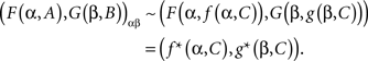
First, selective influence is invariant with respect to all (measurable) transformations of the random variables A,B, even if transformations of A are allowed to depend on values of factor α and transformations of B are allowed to depend on values of factor β. In our example the values of A and B are denoted yes and no. Clearly, we can encode them 0 and 1, respectively, or by any other two numbers or words. Moreover, we can, if we so choose, denote {yes, no} for A by {1, 0} if α = absent but by {−3, 5} if α = present; analogously, we can denote {yes, no} for B by {lion, crocodile} if β = absent but by {zebra, cheetah} if β = present. Selective influence, (A, B) ↫ (α, β), if it holds for the original values for A and B must also hold after any such transformations. This follows from the fact that if (1) holds then after any factor-value-specific transformations F(α, A) and G(β, B) we have

Second, selective influence implies marginal selectivity, the term coined by Townsend and Schweickert (1989) for the situation when the marginal distribution of A does not depend on β and the marginal distribution of B does not depend on α. This is an obvious consequence of (1). The reverse is not true, as illustrated by examples in Dzhafarov (2003) and, more systematically, in Kujala and Dzhafarov (2008). Other examples are given in this paper: in fact, in all our examples where the selective influence relation does not hold marginal selectivity is satisfied.

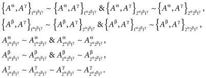
Third, selective influence relation satisfies the nestedness property: if some random variables are selectively influenced by corresponding factors (say, (A, B, C) ↫ (α, β, γ) – we need more than two factor-variable pairs for this property to be non-trivial), then any subset of these variables is selectively influenced by the corresponding subset of factors: (A, B) ↫ (α, β), (A, C) ↫ (α, γ), and (B, C) ↫ (β, z). This property is obvious as soon as (1) is generalized to larger sets.

In this paper the three properties of selective influence will be demonstrated on the maximal level of generality, for arbitrary sets of random entities and corresponding sets of factors of arbitrary nature.

1.3. Distance Tests for Selective Influence

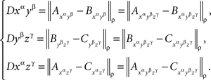
How can one determine that (A, B) ↫ (α, β)? In Kujala and Dzhafarov (2008) two types of necessary conditions for selective influence were formulated, termed cosphericity tests and distance tests. As we only generalize in this paper the latter class of tests, we need not discuss the former. To apply a distance test to our example means to do the following. First, the values of A and B have to be encoded by real numbers. In accordance with what we know about the transformations we can use any functions f(α, A) and g(β, B) with numerical values. Second, one chooses a number ρ ≥ 1. Third, for each of the four treatments αβ = 11, 12, 21, 22 one computes the quantity

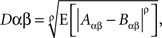
where E denotes expected value and (A_αβ, B_αβ) is an alternative (and more convenient) way of designating (A, B)_αβ. Note that Dαβ (the same as αβ, 21, etc.) is a string of symbols, with no multiplication involved.

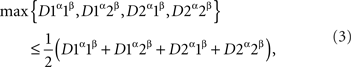
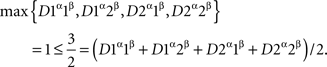
It has been shown in Kujala and Dzhafarov (2008) that if (A, B) ↫ (α, β), then, considering each random variable at each value of the corresponding factor as a point (this yields four points, A₁, A₂, B₁, B₂), these points can be placed in a metric space in which the values D11, D12, D21, D22 are, with some caveats, distances between A points and B points (D11 between A₁ and B₁, D12 between A₁ and B₂, etc.). As these distances, by definition, should satisfy the triangle inequality, we conclude with a bit of algebra (see Section 5) that

A distance test consists in checking if this inequality is satisfied: if not (at least for one choice of the numerical values and the exponent ρ), then the selective influence relation is ruled out.

In this paper we generalize this test to arbitrary sets of random entities selectively influenced by arbitrary sets of external factors. As it turns out, all one has to do to prove that all random entities, taken one for each value of the corresponding factor, can be embedded in a metric space is to apply the test just described to all pairs of 2 × 2 treatments for all pairs of factors. To present this result in an unambiguous form we have to introduce some notation that may appear cumbersome at first: since a value of a factor generally does not itself indicate which factor it is a value of (e.g., absent or 1 can be a value of both α and β), we superscript each factor value by the corresponding factor name. In our example it would be 1^α, 2^α, 1^β, 2^β. We call these pairs, factor value with factor name, factor points. The four distances will now be written D1^α1^β, D1^α2^β, D2^α1^β, D2^α2^β. Note that we could only get away with the previous notation because the identity of the factors in it was encoded by the order of their values within pairs: in D11 the first 1 belonged to α and the second one to β. This convention cannot work, of course, for more than two factors. In the new notation the distance test acquires the form

where

1.4. The Joint Distribution Criterion for Selective Influence

Compliance with a given set of distance tests is only a necessary condition for selective influence. Is there a way to definitively prove that selective influence (A, B) ↫ (α, β) does hold if it is not ruled out by distance tests? As it turns out, the answer is affirmative, and it is an almost immediate consequence of our definition of selective influence, if presented at a sufficiently high level of mathematical rigor. Stated in intuitive terms and applied to our example, consider four hypothetical random variables, one for each of our factor points: 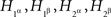. Suppose that they are jointly distributed, i.e., we can speak of co-occurring quadruples of values. There are six pairwise combinations of the four factor points but only four of them, those of the form x^αy^β (x, y ∈{1, 2}), form treatments, whereas the remaining two, 1^α2^α and 1^β2^β, do not. The four treatments correspond to pairs whose joint distributions are well defined. Suppose now that for all those cases when a pair of factor points forms a treatment we have

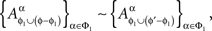
Then and only then (A, B) ↫ (α, β), and we can write then instead of and instead of . We call this the joint distribution criterion for selective influence. The joint distributions of and must also be well defined, even though they do not correspond to any pairs of random variables one can choose from the observable .

Let us look at this in detail. The observed joint distributions of are represented by four probabilities each, denoted in the four matrices introducing our example by p_ij , q_ij , r_ij , s_ij . We now switch to a more convenient notation (although again, more cumbersome at first glance):

where P_ijx^αy^β is a string of symbols, with no multiplication implied. To ascertain if (A, B) ↫ (α, β) using (4), we have to see if we can find 16 probabilities

for four binary variables 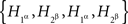, subject to the basic constraints

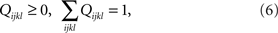
and such that

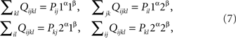
for all i, j, k, l ∈{yes, no}. Indeed,

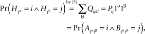
which shows that the first of the equations (7) is equivalent to 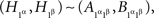the application of (4) to x^αy^β = 1^α1^β; and analogously for the other three equations.

Note that (7) implies marginal selectivity. For instance, it follows from (7) that

and

that is,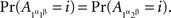

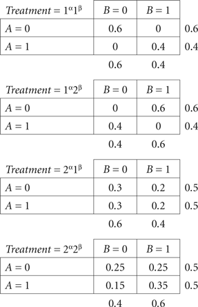
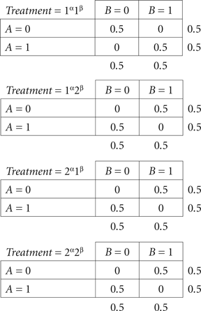
Example 1.1. Let the dependence of {A, B} on {α, β} be described by the distributions

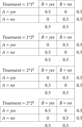
Note that marginal selectivity here is satisfied trivially, as the marginal distributions remain fixed. Consider the distribution of with

It is easy to check that this distribution satisfies (6) and (7), hence also (4). By the joint distribution criterion, we conclude that {A, B} ↫ {α, β}.

Example 1.2. No such probabilities Q_ijkl can be found for the distributions

so {A, B} are not selectively influenced by {α, β} in this case. This can be shown by direct algebra, but there is a simpler method: this dependence of {A, B} on {α, β} fails a distance test. Indeed, let us transform yes into 0 and no into 1, and let us choose the exponent ρ = 1 (although in this example the value of ρ does not matter). Then

and

which contravenes (3).

In this paper the joint distribution criterion is formulated in complete generality, for arbitrary sets of random entities and corresponding sets of external factors.

1.5. The Need for Generalization

In a controlled experiment or systematic survey we usually focus on a small number of random entities, such as which of several responses is given and how long it has taken, and try to selectively target some of them by experimental manipulations, or selectively relate them to concomitant factors. Relatively small networks of random entities and external factors are therefore of paramount practical importance. But a network of random entities and the set of external factors that may be thought to affect them selectively can be quite large, even infinitely large, in theoretical considerations dealing with complex observable behaviors, such as a person’s activities within a typical day, or unobservable “mental networks” behind even relatively simple tasks, such as pushing a key in response to a stimulus varying in two binary properties (see Dzhafarov, Schweickert, and Sung, 2004, for an example). Random processes are routinely used in modeling simple forms of decision making (see, e.g., Diederich and Busemeyer, 2003). Any random process can be viewed as a system of stochastically interdependent random entities indexed by “intervention values” (including “no intervention”) at every moment of time. An intervention α at moment t₁ can be thought to selectively affect a portion of the random process in some interval [t₁, t₂] (perhaps even with t₂ = t₁), and the problem arises as to how to identify such an interval from the observed joint distribution of the random entities constituting the process. It is important therefore to be able to apply the notion of selective influence to arbitrary, finite and infinite, systems of random entities, and external factors.

2. Conventions and Notation

A factor is defined as a non-empty set of factor points (a dummy factor can be defined as a set containing a single point). Denoting factors by lowercase Greek letters, α, β, γ, …, the factor points of, say, factor α are formally pairs (x, ‘α’) consisting of a factor value (or level), x, and a unique factor name, ‘α’ (read: value/level x of factor α). This ensures that no two distinct factors have common points: e.g., level 1 of factor ‘size’ (1, ‘size’), is distinct from level 1 of factor ‘shape’ (1, ‘shape’). It is convenient to write x^α in place of (x, ‘α’): 1^shape, (50 db)^intensity, present^{left stilumus}, etc.

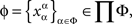
Let Φ be a non-empty set of factors. A set ɸ containing precisely one factor point for each factor α in Φ,

is called a treatment.³ When the set of factors Φ is finite, treatments will be presented as strings of factor points, without commas or parentheses: x^αy^βz^γ, , etc.

Example 2.1. If Φ = {α, β, γ} with α = {1^α, 2^α}, β = {1^β, 2^β}, and γ = {1^γ}, then the treatments ɸ (written as strings) are 1^α1^β1^γ, 1^α2^β1^γ, 2^α1^β1^γ, and 2^α2^β1^γ.

A random entity A is a triad consisting of a measurable function a sample (probability) space and an observation (measurable) space (𝔄, Σ), on which f induces a probability measure M. Traditionally, A is simply identified with f, the sample space and the observation space being assumed implicitly, or A is viewed as the identity function on 𝔄, with (𝔄′, Σ′, M′) = (𝔄, Σ, M). The latter view is often the only practical one, as we almost never know anything about a sample space as separate from the observation space.

A random variable is a random entity whose observation space is a subset of reals endowed with the Borel sigma-algebra.⁴

Given an arbitrary indexing set Ω, any set of random entities whose measurable functions {f_ω:𝔄′→𝔄_ω}_ω∈Ω map from one and the same sample space (𝔄′, Σ′, M′) into respective observation spaces {(𝔄_ω, Σ_ω)}_ω∈Ω possesses a joint distribution, i.e., a probability measure M induced by M′ on the product space ⊗_ω∈Ω(𝔄_ω, Σ_ω).⁵

Example 2.2. Let the sample space consist of 𝔄′ = {0, 1} × {0, 1} × {0, 1}, Σ′ = 2^𝔄′, and M′ derived from elementary probabilities p_ijk (i, j, k ∈{0, 1}). Then the random variables A, B, C defined on (𝔄′, Σ′, M′) by the coordinate projections , , and , respectively (i, j, k ∈{0, 1}), possess the joint distribution M = M′ on ({0, 1}, 2^{0,1}) ⊗ ({0, 1}, 2^{0,1}) ⊗ ({0, 1}, 2^{0,1}) = (𝔄′, Σ′).

Two random entities A and B defined on different sample spaces are called (stochastically or probabilistically) unrelated (see Dzhafarov and Gluhovsky, 2006). They do not possess a joint distribution. Note that two unrelated random variables can be identically distributed – if they map into one and the same observation space on which they induce one and the same probability measure.

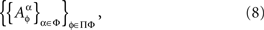
Throughout this paper we deal with a set of probabilistically unrelated random entities {A_ɸ}_ɸ∈ΠΦ indexed by treatments ɸ∈ΠΦ, with measures {M_ɸ}_ɸ∈ΠΦ induced on one and the same observation space (𝔄, Σ). For convenience, we refer to A_ɸ as “a random entity A at ɸ”, as if A_ɸ and for ɸ ≠ ɸ′ were “a single” entity A at two different treatments. Note that A_ɸ and are defined on different sample spaces: they do not possess a joint distribution. In particular, they are not mutually independent.⁶

Example 2.3. The random variables A and B in the examples of Section 1 are called A and B by the abuse of language just mentioned. Strictly speaking we deal with four pairwise stochastically unrelated 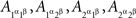and four pairwise stochastically unrelated such that and possess a joint distribution if and only if x^αy^β = z^αu^β.

A set of random entities {A^ω}_ω∈Ω on one and the same sample space is a random entity whose observation space (𝔄, Σ) is the conventionally understood product of the observation spaces (𝔄_ω, Σ_ω) for A^ω, ω ∈ Ω. If the set of random entities {A^ω}_ω∈Ω depends on Φ, we present {A^ω}_ω∈Ω at a treatment ɸ as instead of the more correct but less convenient ({A^ω}_ω∈Ω)_Φ.

Example 2.4. The variables {A, B, C} of Example 2.2 depend on the factors Φ = {α, β, γ} of Example 2.1 if is viewed as a function of ɸ = 1^α1^β1^γ, 1^α2^β1^γ, …. In this example and {a_ɸ, b_ɸ, c_ɸ} = {a, b, c}.

3. Selective Influence

In accordance with the previous section, given a set of factors Φ, a corresponding set of random entities is denoted {A^α}_α∈Φ. For each α∈Φ, the entity A^α may in fact be a shortcut notation for a set of stochastically unrelated random entities indexed by different treatments, In other words, is treated as a random entity A corresponding to factor α and taken at treatment ɸ. The complete notation for the set of random entities {A^α}_α∈Φ then is

where the elements of for a given ɸ, are stochastically interrelated (possess a joint distribution), while the sets and for distinct ɸ, ɸ′, are stochastically unrelated. It is more convenient, however, not to use this explicit notation and to speak instead of {A^α}_α∈Φ depending on Φ.

Definition 3.1. Let a set of random entities {A^α}_α∈Φ indexed by a set of factors Φ depend on this set of factors (i.e., be presentable as (8)). We say that the dependence of {A^α}_α∈Φ on Φ is marginally selective (satisfies the property of marginal selectivity) if, for any subset Φ₁ ⊂ Φ and any ɸ₁∈ΠΦ₁, the distribution of is the same for all treatments ɸ containing ɸ₁ (that is, it does not depend on {x^β∈ɸ : β∈Φ−Φ₁}).

The notion of marginal selectivity was introduced by Townsend and Schweickert (1989), for two random variables. In Dzhafarov (2003) it was generalized to a finite set of random variables under the name of complete marginal selectivity. The adjective “complete” (omitted in the present paper for simplicity) distinguishes this notion from a weaker and less useful generalization of Townsend and Schweickert’s term: for any factor α∈Φ and any treatment ɸ, the distribution of does not depend on {x^β∈ɸ : β∈Φ−{α}}.

Note that Definition 3.1 does not mean that for distinct treatments ɸ and ɸ′ which include ɸ₁ = {x^β ∈ɸ : β ∈Φ₁} = {x^β ∈ɸ′ :β ∈Φ₁},

This equality is not legitimate as the two sets of random variables do not possess a joint distribution. One can only say that

where, as before, ∼ means “is distributed as.”

Example 3.2. Let the variables {A, B, C} of Example 2.2 be indexed by the factors Φ = {α, β, γ} of Example 2.1, respectively. That is, {A, B, C} stands for {A^α, A^β, A^γ}, in accordance with the general notation of Definition 3.1. Then the dependence of {A^α, A^β, A^γ} on {α, β, γ} is marginally selective if and only if

Under marginal selectivity, it is sometimes admissible, by abuse of notation, to write as where ɸ₁ = {x^α ∈ɸ : α ∈Φ₁}. Thus, in Example 3.2, it may be convenient to present both and as present both and as etc. This does not lead to complications provided one remembers that, say, and are identically distributed rather than identical. One can therefore deal with and in all considerations involving only A^α, or with and in all considerations involving only A^β. It would be incorrect, however, to speak of stochastic relationships between or and or to depict such relationships one needs both A^α and A^β to be double-indexed by the factor points involved (unless we have selective influence in addition to marginal selectivity, as explained in the next section).

Example 3.3. Continuing Example 3.2, let us return to writing {A, B, C} instead of {A^α, A^β, A^γ}. We can omit the factor γ when dealing with {A, B} only and write Let the distributions of these random pairs be

We verify that marginal selectivity holds for A and B and introduce the abridged indexing, etc.:

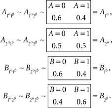
We can use the abridged indexing in all considerations involving A alone and B alone. Consider, however, this: from the joint distribution matrices we have

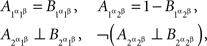
where ⊥ indicates stochastic independence and ¬ negation (i.e., and are not stochastically independent). If now we attempt to use in these relations the abridged indexing, we will run into a contradiction: from and we conclude but then it is impossible for to be independent of and for not to be. It is therefore necessary to retain the notation etc. in all considerations involving both A and B even though we know that the dependence of {A, B} on {α, β} is marginally selective.

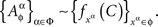
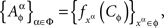
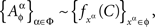
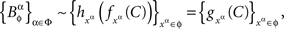
Definition 3.4. Let a set of random entities {A^α}_α∈Φ indexed by a set of factors Φ depend on this set of factors. We say that the set {A^α}_α∈Φ is selectively influenced by Φ, and write

if, for some random entity C and every x^α∈α∈Φ there is a measurable function such that, for every treatment ɸ,

Remark 3.5. Alternatively, one could posit, for every treatment ɸ,

where

is a set of pairwise unrelated random entities all distributed as C. This formulation is more cumbersome but it correctly emphasizes the stochastic unrelatedness of for different treatments ɸ. Definition 3.4, however, is more parsimonious, as the stochastic unrelatedness property is known from the context.

Remark 3.6. If applied to finite sets Φ, Definition 3.4 becomes equivalent to the formulations of selective influence given in Dzhafarov (2003), Dzhafarov and Gluhovsky (2006), and Kujala and Dzhafarov (2008). Even for the finite case, however, the present definition is mathematically more rigorous, and it profits from the precision offered by the notation x^α = (x, ‘α’) for factor points. More importantly, it can be seen more immediately than the previous definitions to be reformulable into the joint distribution criterion for selective influence, as discussed in the next section.

The following statements are obvious.

Lemma 3.7. If {A^α}_α∈Φ↫ Φ, then

(i) for any Φ₁ ⊂ Φ;

(ii) the dependence of {A^α}_α∈Φ on Φ is marginally selective.

That is (refer to Section 1.2), selective influence has the nestedness property and implies marginal selectivity.

The next lemma says that if a set of random entities {A^α}_α∈Φ is selectively influenced by Φ, then the set of individually transformed versions of these random variables is also selectively influenced by Φ (refer to the first property in Section 1.2). “Individual transformations” of A^α can be different for different factor points x^α.

Lemma 3.8. If {A^α}_α∈Φ ↫ Φ then {B^α}_α∈Φ ↫ Φ, where, for any α∈Φ, any x^α∈α, and any treatment ɸ containing x^α,

for some measurable function

Proof. By definition,

which implies

where is a measurable function.                    ☐

4. The Joint Distribution Criterion

Definition 3.4 suggests a way of looking at the selective influence relation directly in terms of the (product) observation space for the system of the random entities involved, making the overt reconstruction of C and the functions unnecessary (or trivial, as in the proof of the theorem below).

Theorem 4.1. A necessary and sufficient condition for

is the existence of a jointly distributed system

such that for every subset ɸ of that forms a treatment (i.e., belongs to ΠΦ),

Remark 4.2. We call this the joint distribution criterion for selective influence.

Proof. The necessity is proved by observing that if {A^α}_α∈Φ ↫ Φ, then the system

is a jointly distributed system of random entities. To prove the sufficiency, define

and, for every x^α, define

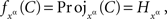
where denotes the x^αth coordinate projection.                    ☐

As a very simple application of the joint distribution criterion we prove the following (intuitively quite obvious) statement.

Lemma 4.3. If the dependence of {A^α}_α∈Φ on Φ is marginally selective and is a set of mutually independent random entities for every treatment Φ, then {A^α}_α∈Φ↫ Φ.

Proof. For any factor α ∈Φ, marginal selectivity implies that the distribution of depends only on the factor point x^α ∈Φ. Form the set consisting of mutually independent random entities such that, for any x^α, Then, for every treatment ɸ, 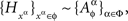and Theorem 4.1 implies {A^α}_α∈Φ↫ Φ. ·     ☐

In Section 1.4 we have seen illustrations of the criterion on interdependent random entities. Here is another example.

Example 4.4. Let Φ = {α, β}, α = {1^α,2^α}, β = {1^β, 2^β}, and let {A_ɸ, B_ɸ} for every treatment ɸ be a pair of Bernoulli variables. Consider the distributions below:

The criterion of the joint distribution of rejects the possibility of {A, B} ↫ {α, β}, as it can be shown by direct algebra that there are no 16 probabilities Q_ijkl generating the distributions in question (cf. Examples 1.1 and 1.2). We do not need to provide such a demonstration as it is obvious in this case from probabilistic considerations that cannot be jointly distributed and satisfy

Otherwise the four joint distribution matrices shown above would have implied, respectively, and , which are not mutually compatible equations.

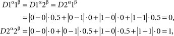
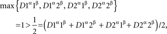
If we take the numerical values of A and B in the last example as they are, then with any exponent ρ ≥ 1 (see Section 1.3) the distance test is passed:

This is just another demonstration that a distance test is only a necessary condition for selective influence: a dependence of random entities on external factors can pass such a test but still fail the joint distribution criterion. It is instructive to see, however, in reference to Lemma 3.8, that with appropriately chosen transformations of the random variables the distributions in question can be made to fail the respective distance tests. Thus, the possibility of selective influence in Example 4.4 will be rejected if we apply the simple transformation

while leaving untransformed. The distributions then become essentially the same as in Example 1.2. The distance tests therefore can be conjectured to have considerable rejection power if one combines it with adeptly chosen transformations (see the open question we pose at the conclusion of the paper). In any case, the exceptional simplicity of these tests makes it worthwhile to always consider them before applying the joint distribution criterion.

5. Distance Tests

In Kujala and Dzhafarov (2008) the distance tests were formulated for two variables influenced by two factors in a two-by-two factorial design. In this section we generalize these tests to arbitrary random variables {A^α}_α∈Φ whose dependence on factors Φ is marginally selective. Perhaps surprisingly, we show that this generalization requires nothing more and nothing less than applying the original tests to all possible two-by-two factorial designs one can extract from Φ.

Distance tests can be applied to non-numerical random entities only after they have been numerically transformed (thus, for the distance test applied to Example 1.2 we transformed yes into 0 and no into 1). In this section therefore we confine our discussion to random variables.

We will need some auxiliary notions and notation conventions. Any finite sequence of factor points is called a chain. Chains will be written as strings, without commas and parentheses (this generalizes the convention we have already used for chains which are finite treatments). Chains can be denoted by capital Roman letters, (from the second half of the alphabet, to distinguish them from random variables and entities for which we use the first half). A chain X may be empty or consist of a single element (factor point), x^α. A subsequence of points belonging to a chain forms its subchain.

A concatenation of two chains X and Y is written as XY. So, we can have chains x^αXy^β, x^αXYy^β, Xx^αy^βY, x^αXy^βZ, etc.

The number of points in a chain X is its cardinality, | X |, and any chain with the smallest cardinality within a set of chains is referred to as a minimal chain (in this set). In particular, one can speak of a minimal subchain of a chain among all subchains with a certain property (this notion is used in the proof of Theorem 5.11 below).

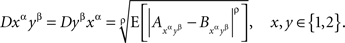
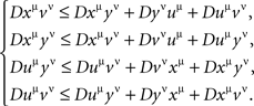
Definition 5.1. Let the dependence of a set of random variables {A^α}_α∈Φ on factors Φ be marginally selective. Let ρ ≥ 1 be fixed. For any (x^α, y^β) with α ≠ β, we define

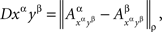
where for any jointly distributed A and B is defined as

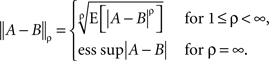
Remark 5.2. Here ess sup is the essential supremum, the lowest upper bound that holds almost surely; it is the limit of as ρ → ∞.

Remark 5.3. Note that Dx^αy^β is well-defined only under the assumption that the dependence of a set of random variables {A^α}_α∈Φ on factors Φ is marginally selective. Otherwise would not be determined by x^αy^β only, and it would not even be legitimate to index the two variables by x^αy^β alone.

We will rely on the following result, whose proof we omit as its only non-trivial part follows from the Minkowski inequality (a somewhat abridged proof can be found in Kujala and Dzhafarov, 2008).

Lemma 5.4. Given a sample space, let ℜ be a set of all random variables A, B, … (jointly distributed) on this space. For any is an extended metric on ℜ, provided we do not distinguish A,B identical on a set of measure 1.

Remark 5.5. The adjective “extended” means that ∞ is included in the set of possible values. The norms and , as they only involve non-negative values, always exist, finite or infinite.

Convention 5.6. In the remainder of this section we will tacitly assume that the dependence of {A^α}_α∈Φ on Φ is marginally selective. We will also tacitly assume that ρ in the definition of and D is fixed.

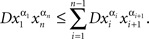
For any chain such that and for i = 1,…,n −1, define

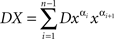
(with the understanding that the sum is zero if n is 0 or 1). The operator D always acts upon the entire chain following it, e.g., .

Definition 5.7. A chain x^αXy^β is said to be compliant with the chain inequality (or simply, compliant) if Dx^αXy^β ≥ Dx^αy^β. The chain is said to be contravening (the chain inequality) if Dx^αXy^β < Dx^αy^β.

It follows from this definition that if x^αXy^β is contravening or compliant, then α ≠ β (otherwise Dx^αy^β is not defined), and no factor in x^αXy^β occurs twice in succession. For a chain to be contravening, in addition, X must be non-empty (i.e., | x^αXy^β | ≥ 3; Lemma 5.9 below shows that in fact | x^αXy^β | ≥ 4). A non-contravening chain need not be compliant: it may, e.g., be any chain with fewer than 3 elements, or it can be any chain of the form x^αXy^α. Analogously, a non-compliant chain is not necessarily contravening.⁷

Lemma 5.8. Let U = Xy^βYz^γZ be a contravening chain with a compliant subchain y^βYz^γ. Then U* = Xy^βz^γZ (i.e., U without Y) is a contravening subchain of U.

Proof. Let x^α and u^δ be the first and the last elements of U, respectively (then necessarily α ≠ δ). Note that x^α may coincide with y^β or u^δ with z^γ (but not both). From

and

we get

Lemma 5.9. Every triadic chain x^αy^βz^γ with pairwise distinct α, β, γ is compliant.

Proof. Denoting the random variables corresponding to the factors α, β, γ, by A, B, C, respectively, marginal selectivity implies

Since 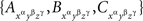are jointly distributed, the statement follows from Lemma 5.4.⁸                                                        ☐

We are ready now to prove the main theorems regarding the distance tests for selective influence.

Theorem 5.10. Let {A^α}_α∈Φ be selectively influenced by Φ. Then any chain such that α_i ≠ α_i+1 for i = 1,…,n − 1, and α₁ ≠ α_n is compliant,

Proof. By the joint distribution criterion, there is a jointly distributed system such that for any {x^α, y^β} within a treatment (i.e. with α ≠ β),

But then

and the statement of the lemma follows from Lemma 5.4.         ☐

For the next theorem, recall that we are following Convention 5.6.

Theorem 5.11. Every contravening chain X contains a contravening tetradic subchain X′ of the form x^αy^βv^αu^β.

Proof. Let X′ = x^αPu^β be a minimal contravening subchain of X. Then α ≠ β, and by Lemma 5.9, | X ′| ≥ 4. If for some z^γ in X′ we had α ≠ γ ≠ β, then the subchains x^αQz^γ and z^γRu^β with Qz^γR = P would have to be compliant (otherwise X′ would not be minimal). Then, by Lemma 5.8, we would have a contravening triadic chain x^αz^γu^β, which is impossible by Lemma 5.9. For every z^γ in X′ therefore, either γ = α or γ = β. Since a contravening chain cannot contain repeating superscripts, X′ is of the form x^αy^βv^αSu^β. But then v^αSu^β must be compliant (otherwise X′ would not be minimal), and by Lemma 5.8 x^αy^βv^αu^β is contravening. Since X′ is minimal, we conclude that S is empty and X′ = x^αy^βv^αu^β.

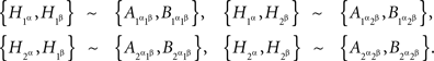
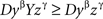
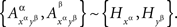
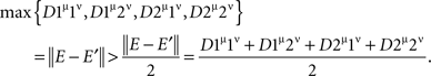
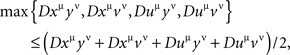
It follows that the task of testing the compliance of D with all possible chain inequalities, as stated in Theorem 5.10, is reduced to testing the compliance with only the inequalities involving tetradic chains: if {A^α}_α∈Φ↫ Φ, then, for any chain x^μy^νu^μv^ν with distinct μ and ν,

and if all such inequalities are satisfied, then there can be no other contravening chains. Given any four factor points x^μ, y^ν, u^μ, v^ν, one can form four different chains with alternating factors and four corresponding inequalities,

Following Kujala and Dzhafarov (2008), these are easy to see (by adding the left-hand sides to themselves and to the right-hand sides) to be equivalent to the single inequality

We call this a tetradic inequality. Note that it is always satisfied if x^μ = u^μ or y^ν = v^ν, so we only have to look at x^μ, y^ν, u^μ, v^ν with two distinct points of each factor.

The theorem below shows that we have to check all such tetradic inequalities (for any given ρ).

Theorem 5.12. The tetradic inequalities are mutually independent, in the sense that any one of them can be violated while the rest of them hold.

Proof. Let μ and ν be distinct factors in Φ, and let, for all points x^μ and y^ν,

where E is some non-singular random variable (i.e., no constant equals E with probability 1). Let 1^μ, 2^μ, 1^ν, 2^ν be distinct fixed points of μ and ν, and let

Let for any point of any factor α ∉{μ, ν} be distributed arbitrarily, and let the random variables be mutually independent for any treatment ɸ, except if the latter includes one of the pairs {1^μ, 2^ν}, {2^μ, 1^ν}, or {2^μ, 2^ν}: in those cases the joint distribution of is given by (9), while and remain the sets of mutually independent variables. It is easy to see that thus defined satisfy the marginal selectivity property.

Now,

where E and E′ are identically distributed and independent. The tetradic inequality on {1^μ, 1^ν, 2^μ, 2^ν} is therefore violated:

Clearly, the tetradic inequality holds on any set {x^α, y^β, s^α, t^β} that does not include {1^μ, 2^ν}, {2^μ, 1^ν}, or {2^μ, 2^ν}, as this inequality then only involves mutually independent random variables (Lemma 4.3 and Theorem 5.10). Denoting by 3^μ any point other than 1^μ and 2^μ (if such a point exists), and analogously for 3^ν, it remains to consider the cases {1^μ, 2^ν, 3^μ, 3^ν}, {1^μ, 2^ν, 2^μ, 3^ν}, {1^μ, 2^ν, 3^μ, 1^ν}, {2^μ, 1^ν, 3^μ, 3^ν}, {2^μ, 1^ν, 1^μ, 3^ν}, {2^μ, 1^ν, 3^μ, 2^ν}, and {2^μ, 2^ν, 3^μ, 3^ν} (note that the order of the points is immaterial here). It is easy to check that the four distances in each of these quadruples equal either 0 or ‖ E − E′ ‖> 0 (with E, E′ independent identically distributed), and that the number of zero distances in these quadruples is never greater than two. The tetradic inequality, therefore, always holds: either

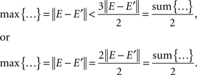
This completes the proof.                                      ☐

Theorem 5.12 is proved for a fixed ρ ≥ 1, and for “untransformed” {A^α}_α∈Φ. The application scope of the distance tests can be significantly broadened by using various values of ρ and by applying to {A^α}_α∈Φ various transformations as specified in Lemma 3.8. It is clear that the tetradic inequalities cannot be independent across all ρ and/or all transformations. Since a violation of a tetradic inequality means a strict inequality, the inequality involving the same quadruple of factor points will have to hold also for sufficiently close values of ρ and sufficiently “slight” transformations. This also applies to ρ = ∞: every violated inequality for ρ = ∞ will have to remain violated for all sufficiently large values of ρ, since the difference between ess sup | A − B | and can be made arbitrarily small (or, if the former is infinite, the latter can be made arbitrarily large).

6. Conclusion

We have advanced the theory of selective influence in three ways.

1. The notion of selective influence (together with the related but weaker notion of marginal selectivity) has been generalized to arbitrary sets of random entities whose joint distributions depend on arbitrary sets of external factors by which the random entities are indexed (Definition 3.4).

2. The joint distribution criterion has been formulated for random entities to be selectively influenced by their indexing external factors: this happens if and only if there is a jointly distributed set of random entities, one for every value of every factor, such that every subset of this set that corresponds to a treatment is distributed as the original entities at this treatment (Theorem 4.1).

3. The distance tests previously formulated for pairs of random variables in two-by-two factorial designs have been generalized to arbitrary sets of random variables. For any quadruple of distinct factor points x^μ, y^ν, u^μ, v^ν, we check whether

where the function D is as in Definition 5.1, for some choice of ρ ≥ 1 and of transformations as specified in Lemma 3.8. If this tetradic inequality is violated, the variables are not selectively influenced by the factors indexing them. It is shown that we do not need to check for compliance with any other chain inequalities (Definition 5.7, Theorems 5.10 and 5.11), and that the tetradic inequalities for different quadruples of factor points (for a given ρ and a given set of transformations) are logically independent (Theorem 5.12).

We conclude by posing an open question. Example 4.4 in Section 4 shows that the distance tests can be passed for all values of ρ while the random variables in question do not selectively depend on the respective factors. At the same time, in this example a distance test can be found to fail after the random variables have been transformed in accordance with Lemma 3.8. The open question is: for random variables which are not selectively influenced (but whose dependence on the corresponding factors is marginally selective), can the distance test be passed under all possible measurable transformations of the variables?

Conflict of Interest Statement

The authors declare that the research was conducted in the absence of any commercial or financial relationships that could be construed as a potential conflict of interest.

Acknowledgments

This research has been supported by NSF grant SES 0620446 and AFOSR grant FA9550-09-1-0252 to Purdue University, as well as by the Academy of Finland grant 121855 to University of Jyväskylä.

Footnotes

1. ^As explained in Section 2, we distinguish random entities and their special case, random variables. Random entities take on values in arbitrary measurable spaces, while random variables map, or can be redefined to map, into real numbers endowed with the Borel sigma-algebra. Note also that the notion of a random entity (or variable) should always be taken to include deterministic entities (variables) as a special case, the same as the notion of stochastic interdependence, unless otherwise indicated, should be taken to include stochastic independence as a special case.
2. ^It is usually the case that the possibility of selectiveness is considered when it is known that the factors are effective in their influence upon (A, B), meaning that for at least one value of either of the two factors the change of the other factor from 1 to 2 changes the joint distribution of (A, B). This aspect of the dependence of (A, B) on (α, β) being relatively trivial, we do not include it in the definition of selective influence. In other words, (A, B) ↫ (α, β) is taken to mean that β does not influence A and α does not influence B, leaving open the question of whether α influences A and/or β influences B (see Dzhafarov, 2003, p. 10).
3. ^Strictly speaking, an element of the Cartesian product ΠΦ is a choice function, whereas a treatment ɸ is the range of a choice function, We conveniently confuse the two notions. Also for convenience only, in this paper we assume “completely crossed design”, i.e., that every member of ΠΦ is a possible treatment. With only slight modifications ΠΦ can be replaced with any nonempty subset thereof.
4. ^A random entity A with 𝔄 a finite or infinite denumerable set and Σ the set of all its subsets can also be (and traditionally is) considered a random variable, because such an 𝔄 can always be injectively mapped into the set of reals, or into a partition of an interval of reals.
5. ^Recall that in the product measurable space ⊗_ω∈Ω(𝔄_ω, Σ_ω) = (𝔄, Σ) the set 𝔄 is the Cartesian product Π_ω∈Ω𝔄_ω, while Σ = ⊗_ω∈ΩΣ_ω is the smallest sigma algebra containing all sets of the form
6. ^We could have extended the scope of this definition by allowing to be a function relating to (𝔄_ɸ, Σ_ɸ), i.e., by allowing the set and the sigma algebra, not only the measure M_ɸ, to depend on treatment ɸ. This would have, however, made our abuse of language (in treating different A_ɸ’s as a single A at different ɸ’s) even more abusive. Moreover, this general approach can always be reduced to the set-up with a ɸ-independent (𝔄, Σ) by putting and Σ the sigma algebra consisting of all countable unions of the sets for all and all ɸ∈ΠΦ.
7. ^We cannot resist mentioning at this point a surprising mathematical similarity between the conceptual apparatus of (hence also the notation adopted in) the present theory, especially in this section, and that of the completely unrelated theory of “regular well-matched spaces” developed in Dzhafarov and Dzhafarov (2010) for comparative judgments. In particular, factors and factor points seem to be formally homologous to “stimulus areas” and “stimuli,” respectively, and the contravening chains of the present theory essentially mirror the “soritical” sequences for comparative judgments, so that the proof of Theorem 5.11 below is almost identical to that of Lemma 3.3 of Dzhafarov and Dzhafarov (2010).
8. ^One can easily generalize this reasoning to show that every chain with pairwise distinct {α₁, … α_n} is compliant. As will be apparent from the proof of Theorem 5.11, however, in the present development we should only be concerned with n = 3.

References

Bloxom, B. (1972). The simplex in pair comparisons. Psychometrika 37, 119–136.

CrossRef Full Text

Diederich, A., and Busemeyer, J. R. (2003). Simple matrix methods for analyzing diffusion models of choice probability, choice response time and simple response time. J. Math. Psychol. 47, 304–322.

CrossRef Full Text

Dzhafarov, E. N. (1997). “Process representations and decompositions of response times,” in Choice, Decision and Measurement: Essays in Honor of R. Duncan Luce, ed. A. A. J. Marley (New York: Erlbaum), 255–278.

Dzhafarov, E. N. (1999). Conditionally selective dependence of random variables on external factors. J. Math. Psychol. 43, 123–157.

Pubmed Abstract | Pubmed Full Text | CrossRef Full Text

Dzhafarov, E. N. (2001). Unconditionally selective dependence of random variables on external factors. J. Math. Psychol. 45, 421–451.

Pubmed Abstract | Pubmed Full Text | CrossRef Full Text

Dzhafarov, E. N. (2003). Selective influence through conditional independence. Psychometrika 68, 7–26.

CrossRef Full Text

Dzhafarov, E. N., and Dzhafarov, D. D. (2010). Sorites without vagueness II: Comparative sorites. Theoria 76, 25–53.

CrossRef Full Text

Dzhafarov, E. N., and Gluhovsky, I. (2006). Notes on selective influence, probabilistic causality, and probabilistic dimensionality. J. Math. Psychol. 50, 390–401.

CrossRef Full Text

Dzhafarov, E. N., Schweickert, R., and Sung, K. (2004). Mental architectures with selectively influenced but stochastically interdependent components. J. Math. Psychol. 48, 51–64.

CrossRef Full Text

Kujala, J. V., and Dzhafarov, E. N. (2008). Testing for selectivity in the dependence of random variables on external factors. J. Math. Psychol. 52, 128–144.

CrossRef Full Text

Lazarsfeld, P. F. (1965). “Latent structure analysis,” in Mathematics and Social Sciences, Vol. 1, eds S. Sternberg, V. Capecchi, T. Kloek, and C. T. Leender (Paris: Mouton), 37–54.

Schweickert, R. (1982). The bias of an estimate of coupled slack in stochastic PERT networks. J. Math. Psychol. 26, 1–12.

CrossRef Full Text

Townsend, J. T. (1984). Uncovering mental processes with factorial experiments. J. Math. Psychol. 28, 363–400.

CrossRef Full Text

Townsend, J. T., and Schweickert, R. (1989). Toward the trichotomy method of reaction times: Laying the foundation of stochastic mental networks. J. Math. Psychol. 33, 309–327.

CrossRef Full Text

Townsend, J. T., and Thomas, R. D. (1994). Stochastic dependencies in parallel and serial models: Effects on systems factorial interactions. J. Math. Psychol. 38, 1–34.

CrossRef Full Text