Multivariate Analysis of Functional Metagenomes

Metagenomics is a primary tool for the description of microbial and viral communities. The sheer magnitude of the data generated in each metagenome makes identifying key differences in the function and taxonomy between communities difficult to elucidate. Here we discuss the application of seven different data mining and statistical analyses by comparing and contrasting the metabolic functions of 212 microbial metagenomes within and between 10 environments. Not all approaches are appropriate for all questions, and researchers should decide which approach addresses their questions. This work demonstrated the use of each approach: for example, random forests provided a robust and enlightening description of both the clustering of metagenomes and the metabolic processes that were important in separating microbial communities from different environments. All analyses identified that the presence of phage genes within the microbial community was a predictor of whether the microbial community was host-associated or free-living. Several analyses identified the subtle differences that occur with environments, such as those seen in different regions of the marine environment.

Introduction

Vast communities of microbes occupy every environment, consuming and producing compounds that shape the local geochemistry. Over the last several years sequence based approaches have been developed for the large-scale analysis of microbial communities. This technique, typically called metagenomics, involves extracting and sequencing the DNA en masse, and then using high performance computational analysis to associate function to each sequence. Annotation of a metagenome is conducted by comparing the sample DNA to that available in various databases, such as NCBI, SEED, MG-RAST, or COG (Wooley et al., 2010). The number of sequences similar to each protein is identified; therefore a metagenome provides information on the taxonomic make up and metabolic potential of a microbial community.

Most of the focus in metagenomics has been on single environments such as coral atolls (Wegley et al., 2007; Dinsdale et al., 2008b), cow intestines (Brulc et al., 2009), ocean water (Angly et al., 2006), and microbialites (Breitbart et al., 2009). Early work compared extremely different environments, like soil microbes compared to water microbes (Tringe et al., 2005). More recently, the Human Microbiome Project has expanded our understanding of the microbes inhabiting our own bodies, comparing samples from the same site among and between individuals (Kurokawa et al., 2007; Turnbaugh et al., 2007, 2009). These studies reflect the dynamic and expanding field of metagenomics which has been reviewed elsewhere (Wooley et al., 2010). Previously, we demonstrated that analysis of functional diversity in metagenomes could differentiate the microbial processes occurring in multiple environments (Dinsdale et al., 2008a). That study utilized the only publicly available metagenomes at that time: 45 microbial samples and 42 viral samples. The raw DNA sequences were compared to the SEED subsystems (Overbeek et al., 2005), and the normalized proportion of sequences in each subsystem in each metagenome were used as the input. That provided a raw data set with 23 response variables and 87 observations (45 microbial metagenomes and 42 viral metagenomes) or samples. In that first study, a canonical discriminant analysis (CDA) was used on a low number of samples from highly disparate environments. In this analysis, we describe a wider range of statistical analyses and use a larger sample size, to describe the abilities of metagenomes to describe the metabolic profile of microbial communities.

Even though metagenomics provides a complete analysis of the microbial activity, the results are complicated to interpret because a typical output is a list of BLAST matches to many thousands of proteins. Some programs for testing significance levels between metagenomes have been written and most use bootstrapping to avoid problems associated with the low number of replicates (Rodriguez-Brito et al., 2006; Parks and Beiko, 2010). Web based sites are being created which enable researchers to conduct statistical analysis, with no explanation of the suitability of the analysis (Arndt et al., 2012). The most common question biologists pose when conducting a metagenomic analysis is how the microbial community taxa or metabolic potential vary between sampling locations or time points. To answer this question requires the analysis and visualization of large amounts of multivariate data. To date, a few statistical tests are routinely used, including principal component analysis (PCA), multidimensional scaling (MDS), and CDA, similar to more traditional analyses of microbial communities and genomic data where PCA dominates the analyses (Ramette, 2007).

There are many statistical tools that can be used to explore multivariate data as provided by metagenomes. Here we provide an overview of seven different statistical techniques, out of the many that could be used, to compare and contrast metagenomes from different environments. In particular, we focus on tools for the classification and visualization of metagenomic data. In this work, we are concerned with how metabolic potential of the microbial community varies within and between environments.

It is important to realize that the statistical tests used will depend on the question the researcher is exploring. Not every statistical test should be used for every analysis, but several analyses can be used in combination to answer the same research question. For example, random forests are a robust analysis, but do not provide a good visualization of the data. Therefore, we combine random forest analysis with either MDS or CDA to visualize the outcome of the random forest. In this work, we have focused on clustering and visualization to show how metagenomes vary between and within environments and identify the metabolic processes that are important in driving the separations. A detailed analysis of the relationship between multivariate analyses can be found in Ramette (2007). Here we take a metagenomes centric view and briefly introduce each statistical method, and describe its ability to separate metagenomes across environmental space.

The analysis recapitulated the discriminating power of metagenomics to identify differences in functional potential both between and within environments. A unique metabolic signature represented each environmental microbial community: for example, the abundance of phage proteins was the major discriminator between host-associated microbial environments and free-living microbes. Subtle differences between open and coastal marine environments were associated with differences in the abundance of photosynthetic proteins. Cofactors, vitamins, and stress related proteins were consistently found in higher abundance in environments where the conditions for microbial survival were potentially unstable, such as hydrothermal springs. Each of these differences provides a clue for detailed microbiological analysis of communities.

Materials and Methods

At the time of analysis, 212 metagenomes were selected from the set of publicly available data¹. They were classified into 10 different environments depending on the description provided by the researcher that collected the samples (Table A1 in Appendix). The metagenomes spanned a range of sequencing technologies, and most environments were represented by two or more sequencing technologies (Figure 1). The sample descriptions were provided as a geographical coordinate or a verbal description (e.g., coral reef water), these were translated into the environmental ontology, EnvO (Smith et al., 2006). EnvO environments were: saline evaporation pond; mat community; hydrothermal springs; human associated; other terrestrial animal associated; freshwater; and marine. Because of the abundance of samples from saline hydrographic features from the ocean (for example, Global Ocean Survey data), these samples were further sub-divided into four groups: open ocean, coastal water, deep water, and coral-reef water associated samples. The descriptions of metagenomes were mostly a geographic location, which would place the sample in a clear habitat type; a description of host, e.g., human or animal type; or a verbal description of the habitat, e.g., hydrothermal springs. There is an unfortunate lack of auxiliary data, e.g., measurements of salinity, pH, temperature, that could be used to separate the samples along a gradient. As more environmental measurements are collected at the time of metagenome sampling, the two data types (environmental and genomic) can be analyzed simultaneously to provide direct evidence of how microbial communities differ across environmental gradients and some of the statistics that we present will useful for these analysis.

FIGURE 1

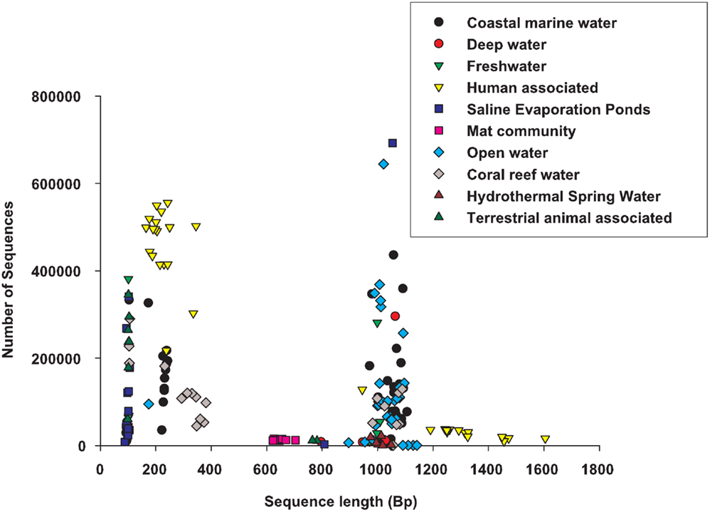
Figure 1. A comparison of the sequence length and number of sequences across the environmental groups.

Publicly available metagenomes were selected from the Edwards Lab metagenome database (see text footnote 1) (Table A1 in Appendix). All samples were annotated using the real-time k-mers based annotation system using a 10-amino acid word size and a requirement for at least two words per protein². Real-time metagenomics: uses signature k-mers to identify the functions encoded in the metagenome sample (Edwards et al., 2012). The k-mers based approach allows all of the samples to be annotated against the same core database, and for the annotations to be updated whenever required. The k-mers based annotation provides the number of sequences for each function, subsystem, and two level hierarchies in the subsystems ontology (Henry et al., 2011). This system works by comparing the DNA to previously annotated DNA housed in a range of databases which identifies a gene or subsystem that shows similarity. The gene is then grouped with other genes that contribute to a metabolic pathway. The pathways are grouped with pathways that are associated with similar metabolic functions to make the top hieratical metabolic function. For example, a sequence may be similar to Alanine racemase, which is used in Alanine Biosynthesis, which is one of the pathways in Amino acid metabolism; therefore in this case the microbial community would have a sequence in the Amino acid metabolism subsystem. The counts for each metabolic process are totaled and normalized by the total number of sequences that show similarity to any subsystem. Therefore the analyses used the percent of sequences in each metabolic or functional group as the data; the metabolic group is the response variable and the metagenomes as the observations. The 27 functional hierarchies used in the analysis were: Amino Acids and Derivatives; Carbohydrates; Cell Division and Cell Cycle; Cell Wall and Capsule; Cofactors, Vitamins, Prosthetic Groups, and Pigments; DNA Metabolism; Dormancy and Sporulation; Fatty Acids, Lipids, and Isoprenoids; Membrane Transport; Metabolism of Aromatic Compounds; Miscellaneous; Motility and Chemotaxis; Nitrogen Metabolism; Nucleosides and Nucleotides; Phages, Prophages, and Transposable Elements; Phosphorus Metabolism; Photosynthesis; Plasmids; Potassium Metabolism; Protein Metabolism; Regulation and Cell Signaling; Respiration; RNA Metabolism; Secondary Metabolism; Stress Response; Sulfur Metabolism; Virulence (Aziz et al., 2008).

Common statistical techniques were used to explore the relationship between the metagenomes, environments, and subsystems (Figure 2). The two key questions addressed were: (i) do metagenomes have a metabolic signature for each environment and (ii) what are the important metabolic processes driving that signature? Clustering analysis is useful for grouping objects into categories based on their dissimilarities and work well when there is discontinuities in the samples, i.e., they are collected from distinct environments, rather than where continuous differences are expected, i.e., they are collected along a single environmental gradient. In general, statistical methods can be divided into two broad categories: supervised techniques and unsupervised techniques. Supervised techniques require that the samples be separated into predetermined groups before the analysis begins, and those groups are used as part of the analytical methods. In this case, the metagenome samples were grouped according to the environment where the sample was collected. In contrast, unsupervised techniques do not require a priori knowledge of the group separations, but the groups are generated by the statistical technique. In the all cases, we compare the resultant groups to the original sampled environment to determine the discriminating power of the analysis.

FIGURE 2

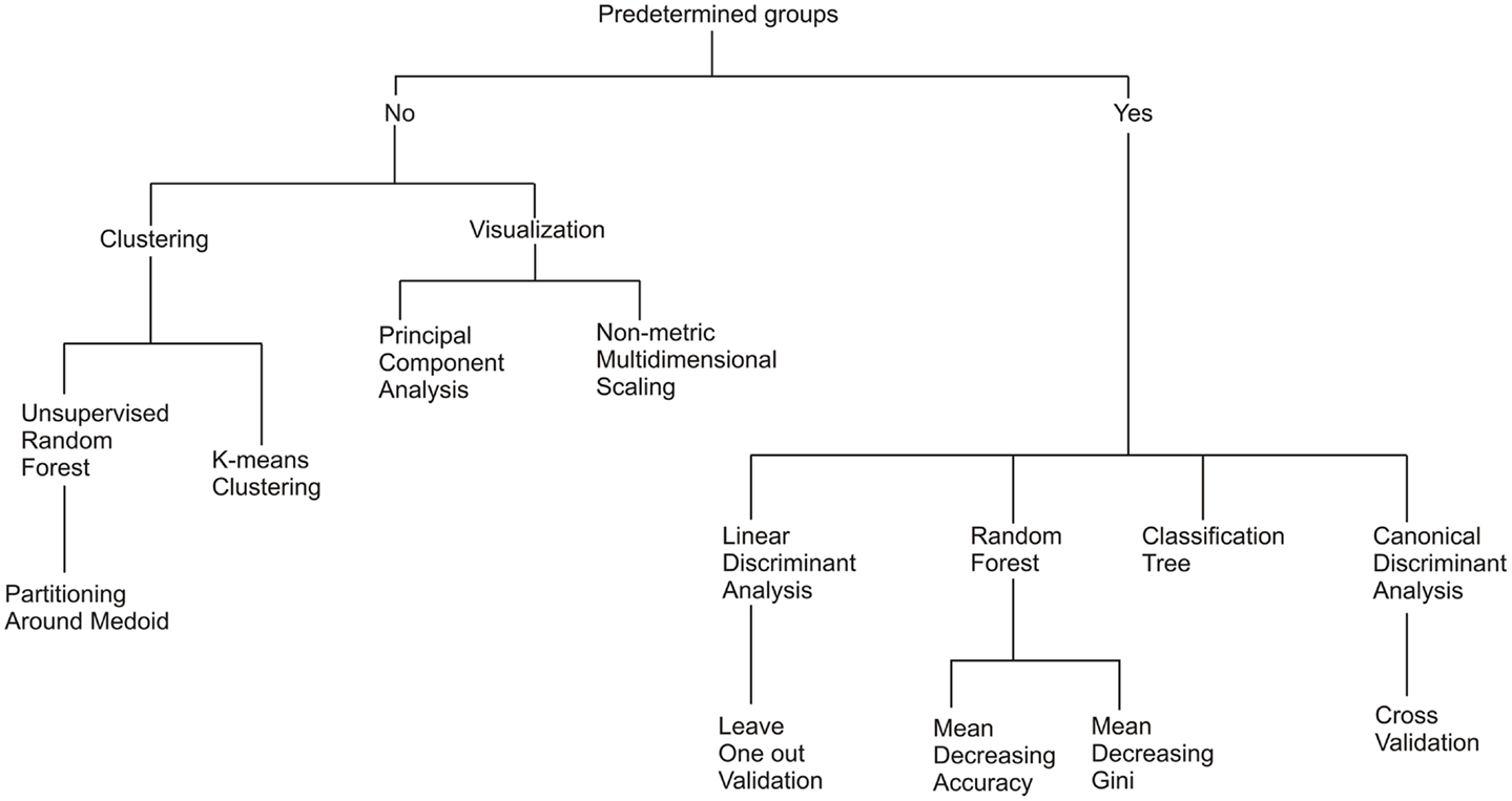
Figure 2. A diagram of the relationship between the seven statistical methods evaluated.

When categorizing data, many statistical methods are prone to over-fitting the data – reading more into the data than is really there. To reduce the problem of over-fitting the size of the data sets should be increased, groups should be of similar size and the number of groups should be less that the number of variables. Sample size considerations are particularly relevant to metagenomic data analysis, due to the nature of the data. There are thousands of proteins identified in each metagenome, but at the time of analysis there were <300 publicly available samples, meaning that there were many less samples than potential variables. Combining the proteins into functional groupings reduces the number of variables to be less than the number of samples available (subsystems were used here, but other groups like COGs, KOGs, or PFAMs are also widely used for metagenome analysis (Reyes et al., 2010). The subsystem approach is standardized and identifies all the proteins that are within a metabolic group. We used BLAST to identify how many sequences are similar to each protein. The data consisted of 10 classifications (the environments), 27 response variables (the functional metabolic groups), and 212 observations (the metagenomes). As the number of publicly available metagenomes increases the number of metabolic groups could be increased. We compared the outcome of the seven statistical analysis with the detailed methods are discussed below, and further discussion and source code for all of these operations are provided in the online accompanying material³. A brief summary of each method is given in the results.

K-means Clustering

K-means clustering is an unsupervised method which aims to classify observations into K groups, for a choice of K. This approach partitions observations into clusters in order to minimize the sum of squared distances from each observation to the mean of its assigned group. The function that is minimized is called the objective function describe in Eq. 1:

$\text{obj}({\mu }_1,\dots ,{\mu }_k)={\displaystyle \sum _{i=1}^n{}_{{\mu }_1,\dots ,{\mu }_k}^{\min }}\Vert x^{(i)}-{\mu }_k\Vert$ (1)

where x⁽ⁱ⁾ is an observation, μ₁, …, μ_k are the means, and k is such that $∥x^{\left(i\right)}-{\mu }_k∥$ is minimal. The result is K clusters where each observation belongs to the cluster with the closest mean.

The K-means algorithm starts by randomly selecting μ₁, …, μ_k and placing all observations into groups based on minimizing the objective function using Euclidean distance. The group means are then recalculated using the observations in each cluster and replace the previous means, μ₁, …, μ_k. The algorithm is repeated until additional runs no longer modify the group means or the partitioning of observations.

An alternative method of choosing K, uses silhouettes (Marden, 2008), which test how well an observation fits into the cluster it has been partitioned into rather than the next nearest cluster. Silhouettes give a good indication of how spread out groups are from each other. Let $a\left(i\right)=∥x^{\left(i\right)}-{\mu }_k∥\text{and}b\left(i\right)=∥x^{\left(i\right)}-{\mu }_l∥$ where x⁽ⁱ⁾ is an observation in group k and l is the group with the next closest mean (Marden, 2008). A silhouette is then defined in Eq. 2:

$\text{silhouette}\left(i\right)=\frac{a\left(i\right)-b\left(i\right)}{max\left\{a\left(i\right),b\left(i\right)\right\}}$ (2)

Ideally, each observation is much closer to the mean of its group than to the mean of any other group. In this case, the silhouette would be close to 1. Similar to the sum of squares plot, one must be careful about choosing a minimal K which has a large average silhouette width, though silhouette graphs frequently suggest a clear K to select.

Cross-Validation of Classification Tree

To cross validate a tree, the data set is divided into k randomly selected groups of near equal size. A large tree is built using the data points in only k − 1 groups and pruned to give a sequence of subtrees. The tree and subtrees are used to predict the classes of the remaining data points, and these predictions are compared against the actual classes of those data points. The misclassification rate and the cross-validated deviance estimate are computed for each tree, and the process is repeated for each group. This k-fold cross-validation procedure (Shi and Horvath, 2006) is typically repeated many times, so that different subsets are selected in each trial. The misclassification and deviance values for each tree size are averaged over there petitions, and the subtree that minimized the standard error in the misclassification rate or the lowest average deviance is selected. Trees constructed using cross-validation tools are typically less susceptible to over-fitting than other forms of classification. K-fold cross-validation is particularly appropriate for metagenomic data where there may be few samples in some of the environmental groups and as many samples as possible should be used to identify the right tree.

Supervised Random Forest Out of Bagging Description

Sampling the data with replacement generates a new dataset to grow each tree in the forest – a process called bagging (bootstrap aggregating). The metagenomes that are chosen at least once during the sampling process are considered in-bag for the resulting tree, while the remaining metagenomes are considered out-of-bag (OOB). Upon mature growth of the forest, each metagenome will be OOB for a subset of the trees: that subset is used to predict the class of the metagenome. If the predicted class does not match the original given class, the OOB error is increased. A low OOB error means the forest is a strong predictor of the environments that the metagenomes come from. Misclassifications contributing to the OOB errors are displayed in a confusion matrix. The rows in the confusion matrix represent the classes of the metagenomes and the columns represent the classes predicted by the subsets of the trees for which each metagenome was OOB. Each class error, weighted for class size, contributes to the single OOB error. The OOB error and a confusion matrix are used to judge the misclassification error and clarify where the errors occur, while the variable importance measure allows for identifying which variables are best at discriminating among groups.

Mean Decreasing Accuracy and Gini in Supervised Random Forest

There are several approaches that work in conjunction with random forests to estimates the importance of variables in separating the data into groups. One uses the mean decrease in accuracy that a variable causes is determined during the OOB error calculation phase. The values of a particular variable are randomly permuted among the set of OOB metagenomes. Then the OOB error is computed again. The more the accuracy of the random forest decreases due to the permutation of values of this variable, the more important the variable is deemed.

The mean decrease in Gini is a measure of how a variable contributes to the homogeneity of nodes and leaves in the Random Forest. Let $p_{m{g}_i}$ be the proportion of samples of group g_i in node m. Let g_c be the most plural group in node m. The Gini index of node mG_m is defined in Eq. 3:

$G_m=1-\sum _{i\in g}{p^2}_{m{g}_i}$ (3)

The Gini index is a measure of the purity of the node, with smaller values indicating a purer node and thus a lesser likelihood of misclassification (Brieiman et al., 1984). Tree generating algorithms may use this index as their likelihood to pick which variable to split on. Each time a particular variable is used to split a node, the Gini indexes for the child nodes are calculated and compared to that of the original node. When node m is split into m_r and m_l, there is a probability $p_{m_r}$ of samples going into the child node m_r and $p_{m_l}$ of going into m_l. The decrease (Brieiman et al., 1984) in Gini is defined inEq. 4:

$D_m=G_m-p_{m_r}{G}_{m_r}-p_{m_l}{G}_{m_l}$ (4)

The calculated decrease is added to the mean decrease Gini for the splitting variable and normalized at the end. The greater the mean decrease Gini of a variable, the purer the nodes splitting. Each time a particular variable is used to split a node, the Gini coefficients for the child nodes are calculated and compared to that of the original node. The Gini coefficient is a measure of homogeneity from 0 (homogenous) to 1 (heterogenous). The decreases in Gini are summed for each variable and normalized at the end of the calculation. Variables that split nodes into nodes with higher purity have a higher decrease in Gini coefficient.

Multidimensional Scaling

Multidimensional scaling is a visualization technique. Its goal is similar to PCA (see below). MDS takes for its input an n × n dissimilarity matrix S for n metagenomes, constructed by some other statistical technique, such as random forest. Then the algorithm looks for an embedding of the data points into some lower (such as 2 or 3) dimensional space that preserves the dissimilarity distances as much as possible. This embedding can then be plotted to visualize the clusters and their distances. There are various algorithms to do this, and they are rather involved. Some try to match the original distances in the embedding as well as it can. Others try to preserve the original ordering of the distances, i.e., the farther apart two samples were originally; the farther apart their images will be under the embedding.

Linear Discriminant Analysis

For a data set with predetermined groups, linear discriminant analysis (LDA) constructs a classification criterion which can be used for predicting group membership of new data. LDA finds linear combinations of variables that best separate the groups, and chooses hyperplanes perpendicular to these vectors to split the data into two groups.

Let X be a data set with defined groups 1, …, n. For each group j, there exists a corresponding conditional distribution describe in Eq. 5.

$X\left(i\right)|G\left(i\right)=j~f_j$ (5)

Furthermore, let π_j represent the proportion of X that is contained in group j. To perform a LDA on X, we assume that each f_j is normally distributed with an equal covariance matrix Σ, but with possibly different means μ_j. Using maximum likelihood estimation theory, the linear discriminant functions can be derived in Eq. 6:

$g_j\left(x\right)=log\left({\pi }_j\right)+x{\Sigma }^{-1}{\mu }_j^T-\frac{1}{2}{\mu }_j{\Sigma }^{-1}{\mu }_j^T$ (6)

Note that π_j, μ_j, and Σ are unknown parameters for our groups’ conditional distributions, so we estimate them using our sample data X in an intuitive manner. Suppose X has N data points and group j has n_j points contained in it. Then we estimate π_j by ${\widehat{\pi }}_j=\frac{n\text{\_}j}{N}$, and μ_j by ${\widehat{\mu }}_j={\displaystyle \sum _{i=1}^n\frac{X_i}{n_j}}$. Let S_j be the sample covariance matrix for group j calculated from X. Also ${\widehat{\Sigma }}_j$, is taken to be 1/n of the pooled covariance matrix of X. Consequently, ${\widehat{\Sigma }}_j={\widehat{\Sigma }}_k$ for all k ∈ {1, …, n}. Therefore, let $\widehat{\Sigma }={\widehat{\Sigma }}_1={\widehat{\Sigma }}_2=\dots ={\widehat{\Sigma }}_k$. With our population parameters estimated from our sample data X, the linear discriminant functions from Eq. 6 becomes described in Eq. 7:

$g_j(x)=\log ({\widehat{\pi }}_j)+x{\widehat{\sum }}^{-1}{\widehat{\mu }}_j^T-\frac{1}{2}{\widehat{\mu }}_j{\widehat{\sum }}^{-1}{\widehat{\mu }}_j^T$ (7)

Note that (5) is a linear function since $log\left({\widehat{\pi }}_j\right)-\frac{1}{2}{\widehat{\mu }}_j{\widehat{\Sigma }}^{-1}{\widehat{\mu }}_j^T$ is a constant.

These g_j’s from (5) are our classifying functions. Since for a point x we sought to maximize π_jf_j, our classification criterion is

$\text{assign\hspace{0.17em}}x\text{\hspace{0.17em}to\hspace{0.17em}group\hspace{0.17em}}j\text{\hspace{0.17em}if\hspace{0.17em}}{g}_j(x)>g_k(x)\text{\hspace{0.17em}for\hspace{0.17em}all\hspace{0.17em}}k\ne j.$

With the classification criterion, decision boundaries between groups can be found. The decision boundaries are where the discriminant functions intersect. That is, the decision boundary between groups j and k is {x:g_j(x) = g_k(x)}. Therefore, the linear discriminant functions split the data space into regions. Each region corresponds to a specific group and the decision boundaries separate the regions.

The original derivation of LDA (Fisher, 1936), the classifier did not start with the multivariate normal distribution. Instead, he sought the linear combination of variables that maximized the ratio of the separation of the class means to the within group variance. The pooled covariance is used in his derivation, which assumes the covariance of the groups is equal. Even though our motivation and derivation are different we still end up with Fisher’s coefficients (Venables and Ripley, 2002).

To judge how well a given LDA acts as a classifier for new data, leave one out cross-validation can be can be used and is implemented in the Statistical Package R (2009). Let X be a data set with m data points, and with groups 1, …, n. For an LDA carried out on X, leave one out cross-validation removes one observation, x⁽ⁱ⁾, at a time from X, performs an LDA on the reduced data set, and then uses this new LDA to classify x⁽ⁱ⁾. Since the group membership of x⁽ⁱ⁾ is already known, we can check if the quasi-LDA for X classifies x⁽ⁱ⁾ correctly or not. For every observation in X, the procedure of leaving one out, and classifying with a new LDA is performed. The number of p of misclassifications is found. The proportion p/m is an estimate for the probability of the LDA carried out on X misclassifying a new observation.

Principal Component Analysis

Principal component analysis is a dimension reduction technique. It uses orthonormal linear combinations of the variables of the data, called principal components, to capture most of the variance in a few dimensions. The idea is to choose the first principal component so that it has maximal variance, and each successive principal component so that it absorbs as much of the remaining variance as possible. The number of principal components of a dataset is equal to the number of variables, but most of the variance is concentrated in the first few.

Given an n × q data matrix Y with corresponding q × q covariance matrix S, the q × 1 principal component vectors ν₁,…, ν_n are described in Eq. 8:

${\langle {\nu }_{\iota },{\nu }_j\rangle }_{\Vert {\nu }_{\iota }\Vert =1}^{{}_{=0,1\le j<i}^{\max }\Vert {\nu }_{\iota }S{\nu }_i^{{\rm T}}\Vert }$ (8)

Since S is a symmetric matrix, the spectral theorem shows that all of its eigenvalues are real and that it has an orthonormal basis of eigenvectors (Marden, 2011). Hence it follows that the principal components of Y are the eigenvectors of S ordered by decreasing eigenvalues.

The principal components of Y capture all of the variance of the variables. PCA is an effective tool when the first few principal components account for most of the variance. In practice, being able to capture over 95% of the variance in the first two principal components is not unusual. Then the data can be plotted along the first two or three principal components to visualize clustering. If the first few principal components fail to account for most of the variance, it indicates that the data is inherently multidimensional.

Canonical Discriminant Analysis

Canonical discriminant analysis centers on the construction of canonical components to explain the variance between classes. For a data set with variables (ν₁, ν₂, … , ν_k), these canonical components are linear combinations of the form shown in Eqs 9 and 10:

$\begin{array}{rc}\text{Can1}& ={\widehat{a}}_1{\nu }_1+{\widehat{a}}_2{\nu }_2+\dots +{\widehat{a}}_k{\nu }_k\end{array}$ (9)

$\begin{array}{rc}\text{Can2}& ={\widehat{b}}_1{\nu }_1+{\widehat{b}}_2{\nu }_2+\dots +{\widehat{b}}_k{\nu }_k\end{array}$ (10)

For two-dimensional visualization it is necessary to project the variable vectors v₁ and v₂, onto the canonical component axes Can1 and Can2 (Marden, 2011). The projections of the variables maintain the relationship between their coefficient variables. That is shown in Eq. 11:

$\frac{a_i}{b_i}=\frac{{\widehat{a}}_i}{{\widehat{b}}_i}\text{and}\frac{a_i}{b_j}=\frac{{\widehat{a}}_i}{{\widehat{b}}_j}$ (11)

The amount of the inter-class variance that is explained by each component is indicated in parentheses along each axis. The vectors can be rescaled to obtain the clearest visualization, but they must maintain the ratio of their lengths as this is proportional to their importance. Each sample is plotted according to its canonical scores. Let x be a sample, such that x = (x₁, x₂, …, x_k) from a data set whose first canonical components are 𝒞₁ and 𝒞₂, such that the coefficients of 𝒞₁ are (a₁, a₂, …, a_k) and those of 𝒞₂ are (b₁, b₂, …, b_k). Then we compute using Eq. 12:

$\begin{array}{llll}x𝒞& =x\left(\begin{array}{c}\hfill |\hfill \\ \hfill {𝒞}_1\hfill \\ \hfill |\hfill \\ \hfill \hfill \end{array}\begin{array}{c}\hfill |\hfill \\ \hfill {𝒞}_2\hfill \\ \hfill |\hfill \\ \hfill \hfill \end{array}\right)=\left(x_1,x_2,\dots ,x_k\right)\left(\begin{array}{c}\hfill a_1\hfill \\ \hfill a_2\hfill \\ \hfill ⋮\hfill \\ \hfill a_k\hfill \\ \hfill \hfill \end{array}\begin{array}{c}\hfill b_1\hfill \\ \hfill b_2\hfill \\ \hfill ⋮\hfill \\ \hfill b_k\hfill \\ \hfill \hfill \end{array}\right)& & \\ & =\left({𝒞}_1\left(x\right){𝒞}_2\left(x\right)\right)\end{array}$ (12)

The canonical scores of a sample x are (𝒞₁(x), 𝒞₂(x)), which describe its position in the 2-dimensional space defined by the first two canonical components. The mean scores and confidence intervals of the means can also be plotted.

The choice of group was determined by the minimal Mahalanobis distance. The Mahalanobis measure is a scale-invariant distance measure based on correlation. The distance of a multivariate vector x = (x₁, x₂, …, x_k) from a group with mean μ = (μ₁, μ₂, …, μ_n) and covariance matrix S is defined in Eq. 13:

$D_M\left(x\right)=\sqrt{\left(x-\mu \right)S^{-1}{\left(x-\mu \right)}^T}$ (13)

More intuitively, consider the ellipsoid that best represents the group’s probability density. The Mahalanobis distance is simply the distance of the sample point from the center of mass, divided by the spread (width of the ellipsoid) in the direction of the sample vector (Marden, 2011).

Results

Overview

We begin by assessing the clustering of the metagenomes and test whether the clusters chosen to reflect the environmental signals are statistically supported (K-means, decision trees, and random forests). We then move on to methods to explore and visualize the underlying structure of the data (MDS, linear discriminant, principal components, and CDA). An outline of the statistical methods tested is shown in Figure 2. Obviously statistical analysis is not a linear process, and many of the techniques were influenced by the results from previous (or subsequent) analyses. Although this discussion attempts to maintain a linear structure for readability, that is not always possible or appropriate. Often the researcher will have a specific biological question and a single specific statistical analysis will be appropriate. A combination of statistical tests can provide better visualization of the data. For example random forests are good at recognizing important variables and how the observations are divided or classified, but do not provide data visualization tools. Therefore, we used a random forest analysis to provide the clustering and a MDS plot to visualize the data.

K-means Clustering

The most straightforward method to cluster data is by grouping into related sets. K-means clustering aims to classify observations into K groups by partitioning observations into clusters in order to minimize the sum of squared distances from each observation to the mean of its assigned group. The K-means algorithm starts by randomly selecting a specified number of means and groups observations by assigning each one to the mean it is closest to in distance. The group means are then recalculated using the observations, replacing the previous means. The observations are reassigned to a group based on the distance between the value and the mean of the group. The algorithm iterates until the groups stabilize. The algorithm will converge to a local minimum, but not necessarily to a global minimum, therefore it is necessary to initialize and run the analysis many times.

Varying the number of groups (K) will result in different results from the K-means algorithm. The sum of squares of distances in general decreases as K increases, because there are more groups in which to assign observations. Selecting K with the smallest sum of squares will over-fit the data. In fact, when K is the number of observations, each observation will form a group by itself and the sum of squares will be 0; but this does not give any useful information about the data. A plot of the sum of squares versus values of K is useful for determining an optimal value of K (Figure 3A). K is often selected where the plot has an “elbow.” However, with metagenomic data, the plot often appeared rounded (Figure 3A), therefore, we optimized using silhouettes (Rousseeuw, 1987) instead. The silhouette of an observation is the difference between its distances from the closest of the K-means and the second closest, divided by its distance from the second closest mean. In the best possible case, the observation is close to its own mean and not very close to the second best mean, i.e., its silhouette is close to 1. The set of all silhouettes (one for each observation) for K from 1 to 10 is shown in Figure 3B. For each value of K we calculate the average silhouette width, and use K that optimizes the width of the silhouettes. We found a maximum at K = 6, with another smaller optimal width at K = 10 (Figure 3C).

FIGURE 3

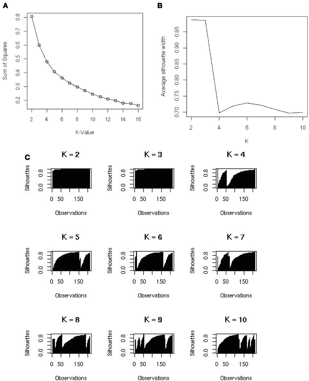
Figure 3. (A) The sums of squares and K-value used to identify the number of groups that the samples should be split into. No clear elbow was evident; therefore silhouette plots were used to examine the data. (B) A silhouette plot showing how it creates metagenomic groups in the data. The most favorable grouping number is where the average silhouette width is nearest to one. (C) The variation of average silhouette width and K. There is a peak at K = 6 and an uptick at K = 10.

The K-means algorithm was most useful for identifying outliers, which could be checked visually and removed as required. Using K = 6 groups, identified two broad categories, (1) the aquatic group cluster and (2) the human, terrestrial animal associated and mat community cluster (Table 1), but the remaining four groups were small and consisted of samples that were potential outliers. The advantage of the K-means approach was that it showed broad patterns in the metagenomic data. If the researcher did not know how many groups were in the dataset, this analysis would be a good place to start the analysis. The disadvantage was that it does not provide any information about which metabolic processes were driving the broad scale separations in the metagenomes.

TABLE 1

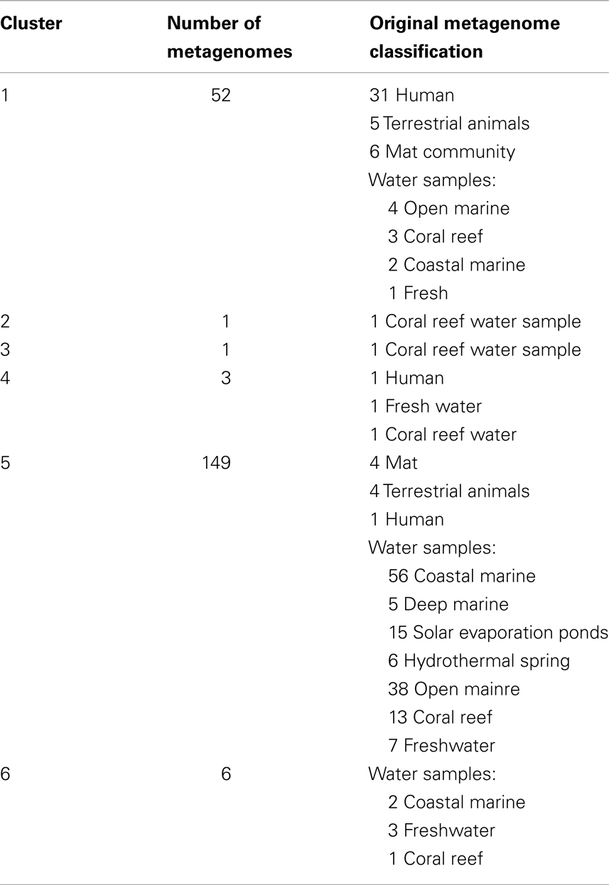
Table 1. The samples present in each of the clusters identified by the K-means analysis with K = 6. This was chosen because the silhouette analysis suggested that six clusters were the most appropriate (Figure 3). There were 33 human, 9 terrestrial animal, 10 mat community, 42 open water, 20 reef water, 60 coastal water, 5 deep water, 7 fresh water, 15 hypersaline, and 6 hot spring samples in total.

Classification Trees

A supervised decision tree constructs a classification tree by identifying variables and decision rules that best distinguish between predefined classes (supervised). If the response variable is continuous, instead of predefined classes, a regression tree can be constructed which predicts the average value of the response variable. Either of these trees is suitable for metagenomic data, but since we were interested in separating the data by environment we used classification trees. Trees are invariant under monotonic transformations of the response variables, because constructing a tree uses binary partitions of the data and thus most variable scaling is unnecessary (De’ath and Fabricius, 2000; De’ath, 2002). This feature is particularly important, because a mixture of data can be included in the analysis, e.g., the percent of sequences similar to a metabolic process or the pH where the metagenome was collected. Combining genomic and environmental data will be useful in future analyses.

The construction of a supervised tree minimizes the mixing of the different predefined classes within a leaf (called the node impurity). At each branching point, the algorithm chooses a single variable and a value that splits the node minimizing the impurity. (There are several ways to measure impurity, as described in the methods) In general, trees are a balance between classification strength and model complexity with the goal of maximizing prediction strength and minimizing over-fitting. Often a large tree is grown that over-fits the data, and pruning and cross-validation are used to select the most appropriate sub-tree of that original tree (Brieiman et al., 1984).

Unlike K-means clustering, decision tree classification provides information about the variables that drive the separation. The best classification tree using all the variables was determined by 500 runs of 10-fold cross-validation (Table 2). The cross-validation identified three trees that gave similarly low values, the 6, 8, and 9-leafed tree. These were visually inspected to see which tree gave information without being over-fitted and this was the 9-leafed tree. This classification tree (Figure 4) demonstrated that phage proteins separated the host-associated microbial communities and the majority of free-living communities. In particular, and as has been shown before (Oliver et al., 2009; Reyes et al., 2010), the host-associated communities and some microbial communities from the fresh water and hypersaline environments characteristically had more phage proteins.

TABLE 2

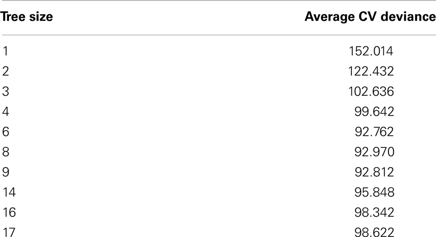
Table 2. Tree size and average deviance from a series of tree cross-validation experiments.

FIGURE 4

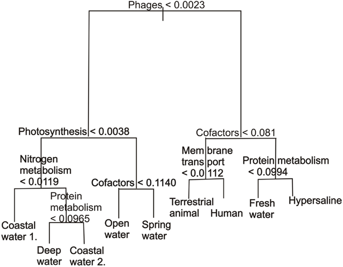
Figure 4. A classification tree showing the separation of metagenomes from different environments based on the abundance of the subsystems in each environment. The abundances are normalized as described in the methods. The tree has been pruned to only show the eight most important variables.

Harsh environments (such as hypersaline aquatic environments) had more cofactors, vitamins, and pigments. Within the marine realm, the coastal and deep water samples had, as expected, fewer photosynthetic proteins than the open water samples, but the photosynthetic potential of the reefs was mixed (Dinsdale et al., 2008a). Photosynthetic potential also aided the identification of stratification in the mat microbial communities by depth, a separation that was supported by metabolism that occurs in microaerobic or anoxic conditions. The major advantages of classification trees are the ability to use any continuous variable type, fast calculation time, good visualization, and the ability to calculate misclassification rate. The use of classification tree in association with environmental data in the future will be able to show the interactions between the environmental and genomic characteristics. The disadvantage is the tendency for over-fitting the trees and the lack of stability: small changes in the data, such as adding one more sample, can yield dramatically different results.

Random Forests

The random forest (Brieiman, 2001) technique aims to overcome the limitations of the classification tree by generating a large ensemble of trees from a random subset of the data and a random selection of the variables. The resulting ensemble of trees (the random forest) is then used with a majority-voting approach to decide which metagenomes belong to which groups. The computation is not excessive: a random forest with 1000 trees trained on 212 metagenome datasets was computed in a few seconds. The speed of calculation and bootstrapping nature of random forests, may pave the way for calculations across all proteins in all environments, thus reducing the amount of grouping conducted on the data. The random forest is typically used to classify the data into predefined groups (a supervised random forest). A subset of the data and variables is used to generate the trees, and thus the approach can predict the environment to which a metagenome belongs. The random forest does not produce branching rules like a single classification tree because the trees in the random forest all differ from one another. Instead, the most parsimonious tree is calculated using bagging (Table A1 in Appendix). In addition to bagging, the RF generates a measure of the importance of each variable, calculated by either the mean decrease in accuracy or the mean decrease in the Gini (Figure 5). These two values indicate which variables contributed the most to generating strong trees and can be used in other visualization analyses such as MDS or CDA as described below.

FIGURE 5

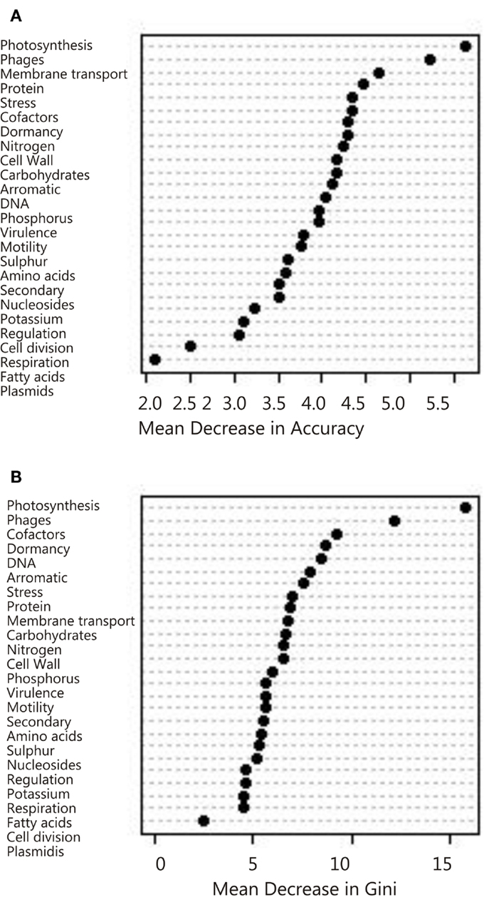
Figure 5. Variable importance determined by the random forest analysis using mean decrease in (A) Accuracy and (B) Gini.

In an unsupervised random forest, the metagenomic data is classified without a priori class specifications. Therefore, unsupervised random forests remove researcher bias. Synthetic classes are generated randomly and the forest of trees is grown. Similar metagenomes will end up in the same leaves of trees due to the tree branching process, and the proximity of two metagenomes is measured by the number of times they appear on the same leaf. The proximity is normalized so that a metagenome has proximity of one with itself and 1-proximity is a dissimilarity measure (Shi and Horvath, 2006). The strength of the clustering detected this way may be measured by a “partitioning around the medoids” (PAM) analysis (Marden, 2011). Conceptually similar to the K-means clustering, PAM picks K metagenomes called medoids, and creates clusters by assigning each metagenome to the group represented by its closest medoid. The algorithm looks for whichever K metagenomes minimize the sum of the distances between all metagenomes and their assigned medoids.

Overall, the photosynthesis and phage groups were the most important response variables in separating the data sets, and in the mean decreasing accuracy plot a break occurred between these two variables and the remaining variables, suggesting that just these two measures could be used to grossly classify the metagenomes (Figure 5). The next break appeared after the eighth variable. These eight variables were thus chosen for the CDA analysis described below. The misclassification rate of the random forest analysis was 31% (Table 3) and these misclassifications occurred because metagenomes from the various marine environments were mixed. The marine environment categories of open ocean, coastal waters, coral reef, and deep ocean, share many metabolic features and therefore these metagenomes were placed into categories different than their a priori group assignment. This suggests subtle variation in metabolic processes that are occurring in the microbial communities from each environment that should be investigated in the future.

TABLE 3

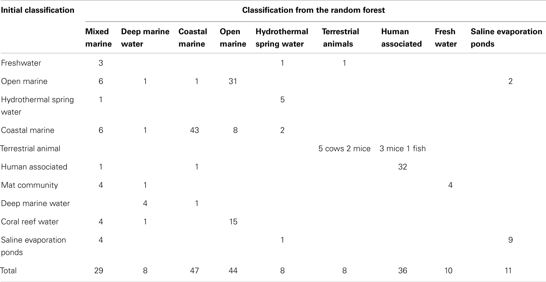
Table 3. The group that each metagenome was assigned to by the random forest analysis.

The advantages of the random forest are that it is a rapid classification technique that is less susceptible to over-fitting data and can be run in a bootstrap fashion. In addition, the random forest provides a measure of the importance of each variable that can be used in other analyses. These advantages of random forests mean that the metagenomes could be analyzed on the gene level, rather than the higher subsystem level. The disadvantage is that because each forest is an ensemble of trees, identifying individual classification decisions is not possible, which is why we plotted the data using a MDS.

Multidimensional Scaling

Multidimensional scaling is a visualization tool that directly scales objects based on either similarity or dissimilarity matrices (Quinn and Keough, 2002). MDS projects the proximity measures of the metagenomes as determined by other techniques to a lower-dimensional space (e.g., 2-dimensional space for plotting on xy-axis). For the random forests, the similarity was measured as the number of times two metagenomes appeared on the same leaf in the trees (proximity), and is represented by the distance between two samples on the MDS plot. The MDS plots are colored either by the five PAM groupings from the random forest (Figure 6A), or the 10 predefined environments (Figure 6B). In this analysis, the visualization highlights the separation of the microbes from human/animal hosts from other samples along the first dimension and the separation of the aquatic and mat communities along the second dimension.

FIGURE 6

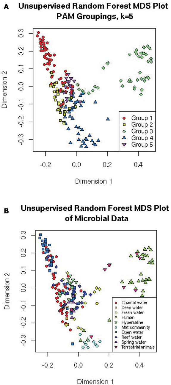
Figure 6. Multiple dimensional scale plots of the distances calculated from the unsupervised random forest. The distances are the number of times the samples appear on the same leaf of the tree, and the MDS has scaled them so that they plot projects those distances into two dimensions. Colored by (A) the five PAM groupings suggested by the random forest (see text); or (B) the original environments the samples came from.

It is important to note that MDS is a visualization technique that takes its input from other classification or clustering approaches. MDS is useful for showing which metagenomes have similar features, because metagenomes that are positioned closer together will be more similar to each other than those farther apart on the plot.

Linear Discriminant Analysis

Linear discriminant analysis is a supervised statistical technique that aims to separate the data into groups based on hyperplanes and describe the differences between groups by a linear classification criterion that identifies decision boundaries between groups.

The LDA over all 27 metabolic variables separated the data (Figure 7) and showed that the human and terrestrial animal associated metagenomes separated from a cluster consisting of all of the aquatic samples except the hypersaline community. The mat samples separated distinctly from the other clusters. A leave one out cross-validation showed that the LDA misclassified 36% of the samples. Most of the misclassified samples were from the aquatic metagenomes that are difficult to separate (as discussed below). Even though it is likely that the data does not meet all the requirements for an LDA, including the assumption of equal population group covariance, a linear function of the variables is still able to separate the groups. We derive the linear discriminant functions assuming the data is normally distributed for simplicity, but this is not necessary. The advantages of LDA are the ability to both visualize the data and obtain a statistically robust classification, but the disadvantage includes the assumption of equal population covariance.

FIGURE 7

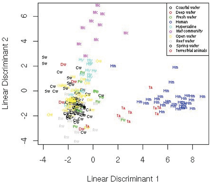
Figure 7. Linear discriminant analysis showing the position of the metagenomes in two-dimensional space from the 10 environments.

Principal Component Analysis

Principal component analysis is one of the most widely used statistical analyses for genomics data because it is a straightforward, robust data reduction technique that is trivial to apply to large data sets. PCA selects linear combinations of the variables sorted so that each combination accounts for as much of the sample variance as possible, while being orthogonal to the previous combinations. These combinations of the variables are called the principal components. The goal of PCA is to explain as much of the variance as possible in the first few components, and thus reduce the complexity of the data by combining related variables. We began with the eight most important variables identified by the random forest, and used PCA to reduce these to a two-dimensional plot. Figure 8 shows a PCA plot of the first two principal components of the data set, and shows the directionality of the importance of each variable.

FIGURE 8

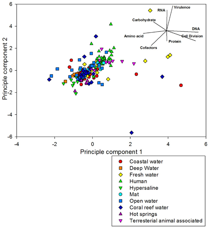
Figure 8. Principal component analysis of the 212 metagenomes using the top eight variables identified from the random forest analysis. The samples are colored and shaped by the environment where they came from. The samples are largely aligned on a 45° plane from virulence-DNA metabolism to amino acids-cofactors.

The data was positioned on a plane which was influenced by a high percent of sequences associated with DNA metabolism, cell division, and amino acid metabolism in one direction, and virulence and RNA metabolism in the other, with cofactor metabolism important in both directions. The metagenomes did not separate particularly well with this analysis, however human and terrestrial animal associated samples clustered above aquatic samples. The first two dimensions of the PCA did not provide good resolution of the nuances within an environment, explaining only 38% of the variance. This suggests that a large number of components were needed to explain the variance in our data and highlights a problem with PCA: it is not able to reduce the complexity of the data if the variables are not correlated. The lack of correlation in the variables can be seen in Figure 8, because the metabolic processes are facing in different directions around the graph. There is no grouping of any of the 8 metabolic processes shown. We did get better resolution with PCA on certain subsets of the data for example, using some of the organism-associated metagenomes. In this case the first two principal components accounted for 79% of the variance. We did not include those graphs in this paper.

The advantages of the PCA are that it reduces the complexity of the data, especially if many of the variables are correlated, and it provides a mechanism for visualizing higher-dimensionality data. The disadvantages of the PCA are that it does not classify the metagenomes into groups and if the variables are not correlated it is unable to reduce the dimensionality of the data.

Canonical Discriminant Analysis

Canonical Discriminant Analysis is another approach to reduce the dimensionality of the data, similar to PCA and LDA. However, in addition to visualizing the data, CDA can be used to classify the data into pre-assigned groups. Like the PCA, CDA searches for linear combinations of variables that explain the data. Like a supervised random forest, CDA can be used to explore the variables responsible for differentiating between groups.

CDA identifies variation between groups by identifying the linear combination of variables that has the maximum multiple correlations with the groups. The second component is the linear combination that has the highest possible multiple correlations within the groups and is uncorrelated with the first component. The process is repeated using all the data, and providing one fewer components than variables. A fundamental difference between PCA and CDA is the covariance matrix: in the former the covariance matrix displays the variance between individual samples, while in the latter it displays the variance between groups. As with the PCA, we explored the effect of the eight most important response variables on the separation of the 212 metagenomes using CDA (Figure 9) and found the mediods of the groups and vectors that demonstrate the directionality of the importance of each variable. The length of the vector in the plot is proportional to the importance of that variable in separating the data.

FIGURE 9

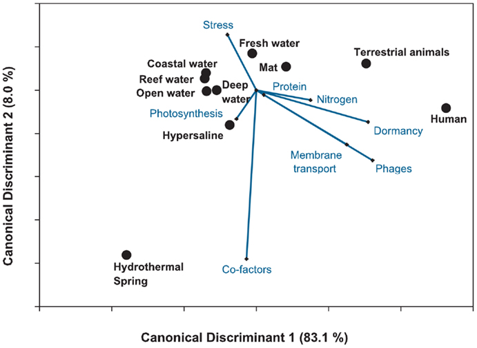
Figure 9. Canonical discriminant analysis of the 212 metagenomes using the top eight variables identified from the random forest analysis. The plot shows the separation in the host-associated microbial communities and the free-living communities. The analysis explained 91% of the variance, suggesting that metagenomes can be discriminated by the metabolic potential. Lines depict the h-plot of important metabolic processes and the points are the centroid or mean for the 10 environments.

The CDA showed that the host-associated microbial communities were separated from the other environments by the abundance of sequences similar to phage and dormancy proteins. The harsh hydrothermal springs were again associated with the need for cofactors. The photosynthetic potential separated the coastal and open water metagenomes. Membrane transport, protein and nitrogen metabolism were also important in separating the aquatic from host-associated metagenomes. The analysis explained a large amount of the variance (91%) showing the importance of a key set of metabolic processes in each environment. However, the misclassification rate of the CDA was 39.7%. Once again the largest misclassification occurred between the metagenomes collected from the four marine environments (Table 4).

TABLE 4

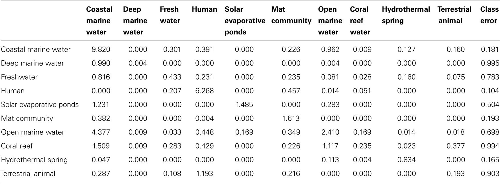
Table 4. The misclassification table generated by the canonical discriminant analysis.

The advantages of the CDA are that it combines the dimensionality reduction of the PCA with the classification of the random forest or K-means approaches. The disadvantages of the CDA are that the metagenomes are placed into predefined groups and thus are subject to observer bias, and CDA is prone to over-fitting because the canonical components are linear combinations that best separate the groups.

Discussion

Metagenomic data provides a wealth of information about the functional potential of microbial communities, but the vastness of the data makes it difficult to discern patterns and important discriminators. A range of clustering, classification and visualizing techniques were applied to analyze metagenomic data, and demonstrated the ability of the metabolic profiles to describe the difference between environments. The results show that a mixture of methods provides an effective analysis of the data: K-means was used to identify outliers, random forests to identify the most important variables, and either a classification tree or CDA to test the relevance of the environment to genomic content.

The data generation processes could cause differences in the classification or separation of the data. However the samples came from multiple sources, each of which employed a range of isolation, purification, and sequencing techniques. There was no evidence of clustering of samples prepared or sequenced in a specific manner, suggesting that the sampling technique per se is not driving the separation of the data.

The analyses separated the microbial samples into three broad groups (based on the environments from where they were isolated): the human and animal associated samples, the microbial mats, and the aquatic samples. There was a clear difference between environments. For example, human associated and aquatic samples were clearly separated by all of the techniques. However, samples from a similar environment were often misclassified. For example, the coastal and open water metagenomes were difficult to classify. More sampling and more thorough description of the environmental parameters will clarify the classification of these samples.

The combination of random forests and CDA demonstrated that phage activity is a major separator of host-associated microbial communities and free-living or environmental microbial communities, suggesting that the phages are playing different ecological roles within each environment. In free-living microbial communities, phages are major predators and generally show similar diversity to their hosts. In host-associated microbial communities, phages are more diverse suggesting that they may provide specific genes to increase host survival (Reyes et al., 2010). The mat communities separated from both the animal associated metagenomes and the aquatic samples by the vitamin and cofactor metabolism, suggesting a role for secondary metabolism associated with growth in extreme environments. The dominant metabolism that separated the aquatic samples was photosynthesis. Not surprisingly, samples from deep in the ocean, and some of the impacted reef sites, do not have many photosynthetic genes, while photosynthetic genes abound on unaffected reefs and in surface waters of the open ocean. Although only the one or two most abundant phenotypes in each sample were described here, the statistical analysis reveals less obvious separations among the data, and unraveling the role of microbes in the global geobiology is an important goal for post-metagenomic studies.

In summary, we hope that the statistical tools described here will help microbial ecologists broaden the range of statistical tools that are used in metagenomic data and help them parse out the important and interesting nuances that separate different environments.

Conflict of Interest Statement

The authors declare that the research was conducted in the absence of any commercial or financial relationships that could be construed as a potential conflict of interest.

Acknowledgments

This work was supported by the NSF REU grant from the NSF Division of Mathematical Sciences (NSF DMS-0647384) to Vadim Ponomarenko (Research Experience for Undergraduates Student Participants: Naneh Apkarian, Michelle Creek, Eric Guan, Mayra Hernandez, Katherine Isaacs, Chris Peterson, Todd Reght, REU Instructors: Imre Tuba, Barbara A. Bailey, Robert A. Edwards, Elizabeth A. Dinsdale). Students conducted all of the analysis and wrote scripts for R. Elizabeth A. Dinsdale was supported by a grant from the NSF Transforming Undergraduate Education and Science (NSF TUES-1044453). Robert A. Edwards was supported by the PhAnToMe grant from the NSF Division of Biological Infrastructure (NSF DBI-0850356).

Footnotes

1. ^http://edwards.sdsu.edu/mymgdb/
2. ^http://edwards.sdsu.edu/rtmg
3. ^http://dinsdalelab.sdsu.edu/metag.stats/

References

Angly, F., Felts, B., Breibart, M., Salamon, P., Edwards, R. A., Carlson, C. A., et al. (2006). The marine viromes of four oceanic regions. PLoS Biol. 4:e368. doi:10.1371/journal.pbio.0040368

Pubmed Abstract | Pubmed Full Text | CrossRef Full Text

Arndt, D., Xia, J. G., Liu, Y. F., Zhou, Y., Guo, A. C., Cruz, J. A., et al. (2012). METAGENassist: a comprehensive web server for comparative metagenomics. Nucleic Acids Res. 40, W88–W95.

Pubmed Abstract | Pubmed Full Text | CrossRef Full Text

Aziz, R. K., Bartels, D., Best, A. A., Dejongh, M., Disz, T., Edwards, R. A., et al. (2008). The RAST server: rapid annotations using subsystems technology. BMC Genomics 9:75. doi:10.1186/1471-2164-9-75

CrossRef Full Text

Breitbart, M., Hoare, A., Nitti, A., Siefert, J., Haynes, M., Dinsdale, E., et al. (2009). Metagenomic and stable isotopic analyses of modern freshwater microbialites in Cuatro CiEnegas, Mexico. Environ. Microbiol. 11, 16–34.

Pubmed Abstract | Pubmed Full Text | CrossRef Full Text

Brieiman, L. (2001). Random forests. Mach. Learn. 45, 5–32.

CrossRef Full Text

Brieiman, L., Friedman, J. M., Stone, C. J., and Olshen, R. A. (1984). Classibication and Regression Trees. Boco Raton: Chapman and Hall CRC.

Brulc, J. M., Antonopoulos, D. A., Miller, M. E. B., Wilson, M. K., Yannarell, A. C., Dinsdale, E. A., et al. (2009). Gene-centric metagenomics of the fiber-adherent bovine rumen microbiome reveals forage specific glycoside hydrolases. Proc. Natl. Acad. Sci. U.S.A. 106, 1948–1953.

Pubmed Abstract | Pubmed Full Text | CrossRef Full Text

De’ath, G. (2002). Multivariate regression trees: a new technique for modeling species-environment relationships. Ecology 83, 1105–1117.

CrossRef Full Text

De’ath, G., and Fabricius, K. E. (2000). Classification and regression trees: a powerful yet simple technique for ecological data analysis. Ecology 81, 3178–3192.

CrossRef Full Text

Dinsdale, E. A., Edwards, R. A., Hall, D., Angly, F., Breitbart, M., Brulc, J. M., et al. (2008a). Functional metagenomic profiling of nine biomes. Nature 452, U628–U629.

CrossRef Full Text

Dinsdale, E. A., Pantos, O., Smriga, S., Edwards, R. A., Wegley, L., Angly, F., et al. (2008b). Microbial ecology of four coral atolls in the northern line islands. PLoS ONE 3:e1584. doi:10.1371/journal.pone.0001584

CrossRef Full Text

Edwards, R. A., Olson, R., Disz, T., Pusch, G. D., Vonstein, V., Stevens, R., et al. (2012). Real time metagenomics: using k-mers to annotate metagenomes. Bioinformatics 28, 3316–3317.

Pubmed Abstract | Pubmed Full Text | CrossRef Full Text

Fisher, R. A. (1936). The use of multiple measurements in taxonomic problems. Ann. Eugen 7, 179–188.

CrossRef Full Text

Henry, C. S., Overbeek, R., Xia, F. F., Best, A. A., Glass, E., Gilbert, J., et al. (2011). Connecting genotype to phenotype in the era of high-throughput sequencing. Biochim. Biophys. Acta 1810, 967–977.

Pubmed Abstract | Pubmed Full Text | CrossRef Full Text

Kurokawa, K., Itoh, T., Kuwahara, T., Oshima, K., Toh, H., Toyoda, A., et al. (2007). Comparative metagenomics revealed commonly enriched gene sets in human gut microbiomes. DNA Res. 14, 169–181.

Pubmed Abstract | Pubmed Full Text | CrossRef Full Text

Marden, J. (2011). Multivariate Statistical Analysis Old School. Available at: http://istics.net/pdfs/multivariate.pdf.

Marden, J. I. (2008). Multivariate Statistical Analysis Old School [Online]. Available at: http://www.lulu.com

Oliver, K., Degnan, P., Hunter, M., and Moran, N. (2009). Bacteriophages encode factors required for protection in a symbiotic mutualism. Science 325, 992–994.

Pubmed Abstract | Pubmed Full Text | CrossRef Full Text

Overbeek, R., Begley, T., Butler, R. M., Choudhuri, J. V., Chuang, H. Y., Cohoon, M., et al. (2005). The subsystems approach to genome annotation and its use in the project to annotate 1000 genomes. Nucleic Acids Res. 33, 5691–5702.

Pubmed Abstract | Pubmed Full Text | CrossRef Full Text

Parks, D. H., and Beiko, R. G. (2010). Identifying biologically relevant differences between metagenomic communities. Bioinformatics 26, 715–721.

Pubmed Abstract | Pubmed Full Text | CrossRef Full Text

Quinn, G. P., and Keough, M. J. (2002). Experimental Design and Data Analysis for Biologists. Cambridge: Cambridge University Press.

Ramette, A. (2007). Multivariate analyses in microbial ecology. FEMS Microbiol. Ecol. 62, 142–160.

Pubmed Abstract | Pubmed Full Text | CrossRef Full Text

Reyes, A., Haynes, M., Hanson, N., Angly, F. E., Heath, A. C., Rohwer, F., et al. (2010). Viruses in the faecal microbiota of monozygotic twins and their mothers. Nature 466, U334–U381.

CrossRef Full Text

Rodriguez-Brito, B., Rohwer, F., and Edwards, R. (2006). An application of statistics to comparative metagenomics. BMC Bioinformatics 7:162. doi:10.1186/1471-2105-7-162

Pubmed Abstract | Pubmed Full Text | CrossRef Full Text

Rousseeuw, P. J. (1987). Silhouettes – a graphical aid to the interpretation and validation of cluster-analysis. J. Comput. Appl. Math. 20, 53–65.

CrossRef Full Text

Shi, T., and Horvath, S. (2006). Unsupervised learning with random forest predictors. J. Comput. Graph Stat. 15, 118–138.

CrossRef Full Text

Smith, B., Kusnierczyk, W., Schober, D., Ceusters, S., and Werner, C. (2006). “Towards a reference terminology for ontology research and development in the biomedical domain,” in Proceedings of KR-MED, ed. O. Bodenreider Baltimore, 57–66.

Statistical Package, R. (2009). R: A Language and Environment for Statistical Computing. Vienna, Austria: R Foundation for Statistical Computing.

Tringe, S. G., Von Mering, C., Kobayashi, A., Salamov, A. A., Chen, K., Chang, H. W., et al. (2005). Comparative metagenomics of microbial communities. Science 308, 544–557.

CrossRef Full Text

Turnbaugh, P. J., Hamady, M., Yatsunenko, T., Cantarel, B. L., Duncan, A., Ley, R. E., et al. (2009). A core gut microbiome in obese and lean twins. Nature 457, U480–U487.

CrossRef Full Text

Turnbaugh, P. J., Ley, R. E., Hamady, M., Fraser-Liggett, C. M., Knight, R., and Gordon, J. I. (2007). The human microbiome project. Nature 449, 804–810.

Pubmed Abstract | Pubmed Full Text | CrossRef Full Text

Venables, W. N., and Ripley, B. D. (2002). Modern Applied Statistics with S. New York: Springer.

Wegley, L., Edwards, R. A., Rodriguez-Brito, B., Liu, H., and Rohwer, F. (2007). Metagenomic analysis of the microbial community associated with the coral Porites astreoides. Environ. Microbiol. 9, 2707–2719.

Pubmed Abstract | Pubmed Full Text | CrossRef Full Text

Wooley, J. C., Godzik, A., and Friedberg, I. (2010). A primer on metagenomics. PLoS Comput. Biol. 6:e1000667. doi:10.1371/journal.pcbi.1000667

Pubmed Abstract | Pubmed Full Text | CrossRef Full Text

Appendix

TABLE A1

Table A1. Metagenomes used in the analysis.