Integration of the ImageJ Ecosystem in KNIME Analytics Platform

Introduction

In the field of bioimage analysis, a wide range of software tools have been published that tackle a wide range of bioimage processing and analysis tasks. While these tools vary widely in their target audiences and implementations, many of them are open-source software (Eliceiri et al., 2012) due to the many advantages it brings to science (Cardona and Tomancak, 2012).

ImageJ is among the most popular open-source image analysis platforms in the community (Schindelin et al., 2015). The platform is divided into multiple parts, including an end-user application (“the ImageJ application”) commonly used by scientists and a suite of software libraries (“the ImageJ libraries”) that perform the underlying image analysis operations. The ImageJ application is a standalone image processing program in development since 1997 (Schneider et al., 2012) and is designed for scientific images. It is highly extensible, with thousands of plugins and scripts for performing a wide variety of image processing tasks contributed by community developers. The Fiji distribution of ImageJ (Schindelin et al., 2012) bundles ImageJ in a combined application together with useful plugins focused on the life sciences. In recent years, ImageJ and Fiji developers have invested much effort in improving the software's internals, redesigning the ImageJ libraries to improve robustness, scalability, and reproducibility across a broader range of n-dimensional scientific image data (Rueden et al., 2017, p. 2).

The paradigm of the ImageJ application fundamentally centers around images as the primary data upon which all commands operate. ImageJ excels at exploratory single-image processing: the user opens an image file and then applies various processing and analysis actions, receiving rapid feedback on the consequences of those operations. To solidify a sequence of actions that achieves an effective analysis and apply that sequence across many images, a writing code is essential. Typically, the user invokes ImageJ's Macro Recorder feature (https://imagej.net/Recorder) to generate a series of code snippets corresponding to manually performed operations and then assembles and generalizes these snippets into a script that can then repeat those same operations on even more images (https://imagej.net/Batch). These scripts can be reused in a variety of contexts—e.g., from the command line or within the ImageJ application via the Process › Batch submenu—but they are linear in execution and limited in scale, requiring more complex programming techniques to fully utilize computational resources across multiple cores, graphics processing units (GPUs), or machines on a cluster—especially for images exceeding ImageJ's historical size limits (i.e., maximum 2 gigapixels per image plane).

Even with a script to perform analyses at scale across many images, ImageJ application users must take care to avoid pitfalls relating to reproducibility of algorithm execution. Numerical results may differ based on ImageJ's settings—e.g., should 0 values be treated as background or foreground?—as well as across versions of ImageJ and its myriad of extensions. A script written in ImageJ's macro language can declare a minimum version of the core ImageJ software it needs to execute, but it must be specified manually, as the exact versions of ImageJ plus installed extensions are not recorded anywhere. Savvy users could do so manually and then take care to publish the configurations used for their analyses, but ImageJ does not provide convenient means of reconstructing such environments.

Versioning becomes even more difficult when considering extensions, which are distributed via ImageJ update sites (https://imagej.net/Update_Sites). Currently, with multiple update sites enabled in an ImageJ installation, there is no mechanism in place to ensure compatibility between the sites. As such, workflows requiring complex combinations of update sites—which are then themselves often shared via update sites also—are in danger of being irreproducible across installations, especially as the required extensions evolve over time.

Some of these issues can be overcome in time with technical efforts to improve the ImageJ platform—e.g., a future version of ImageJ could offer parallel execution as an option within the relevant batch commands—but the ImageJ interface's treatment of individual images as primary datasets will always impose certain challenges when attempting to produce investigation-focused scientific workflows. Investigators often combine classical image processing techniques with leading-edge algorithms from the field of deep learning, machine learning, and data mining, as well as established statistical analysis and visualization methods, to solve a great variety of image analysis problems. Unfortunately, ImageJ's selection of tools outside image processing—e.g., machine learning or statistical analysis of results—is substantially less complete than its suite of image processing commands.

An effective strategy for overcoming limitations of a particular software tool is the integration with other complementary tools (Carpenter et al., 2012). Integrating multiple tools enables a broad range of functionality and algorithms, not only to analyze images but also for the subsequent statistical evaluation and visualization of the numbers extracted from them. In recent years, ImageJ has been adapting to the community's need for interoperability by changing from a monolithic software application into a highly modular software framework, fostering its integration and reusability from other open-source platforms (Rueden et al., 2017, p. 2).

The KNIME Image Processing extension (Dietz and Berthold, 2016) leverages these efforts and integrates ImageJ's extensive functionality into the KNIME open-source product known as KNIME Analytics Platform (Berthold et al., 2008). The open-source KNIME Analytics Platform has been created and extended by academic and industrial researchers across several disciplines such as cheminformatics (Mazanetz et al., 2012; Beisken et al., 2013) and mass spectrometry (Aiche et al., 2015) to provide a framework for seamlessly integrating a diverse and powerful collection of software tools and libraries. It is now a widely used, user-friendly data integration, processing, analysis, and exploration platform, designed to handle huge amounts of heterogeneous data and making state-of-the-art computational methods accessible to non-experts. Therefore, utilizing the ImageJ libraries from within KNIME Analytics Platform not only enables researchers to build scalable, reproducible, image analysis workflows, but it also allows them to combine ImageJ with a variety of extensions from various domains readily available in KNIME Analytics Platform, including machine learning, deep learning, statistical analysis, data visualization, and more.

In contrast to more loosely coupled scientific workflow management systems such as Galaxy (Afgan et al., 2018), KNIME Analytics Platform uses a more tightly coupled approach, with shared strongly typed data structures (Wollmann et al., 2017). The KNIME Image Processing extension uses ImageJ's foundational libraries as the core of its Image Processing extension, reusing the exact same algorithm implementations, avoiding reinventing the wheel. At the heart of this effort is ImageJ Ops (henceforth referred to as “Ops”), an extensible library of image processing operations. Ops includes many common image processing algorithms, including arithmetic, morphology, projection and scaling, statistics, thresholding, convolution, Fourier transforms, and many more. Both ImageJ and the nodes of the KNIME Image Processing extension make use of Ops, enabling users to take advantage of both worlds seamlessly. Image processing algorithms implemented in Ops are usable directly from any SciJava-compatible software project (https://imagej.net/SciJava), such as ImageJ, KNIME Analytics Platform, and the OMERO image server (Allan et al., 2012).

In this paper, we demonstrate several ways of utilizing ImageJ functionalities within KNIME workflows. We will also highlight real-world biological examples that take advantage of commonly used ImageJ tools and plugins, such as TrackMate (Tinevez et al., 2017) and Trainable Weka Segmentation (Arganda-Carreras et al., 2017), as applied within the KNIME workflows. The goal of this paper is to demonstrate how ImageJ users and developers can use KNIME Analytics Platform to create scalable and reproducible scientific workflows combining ImageJ with a broader ecosystem of analysis tools.

Results

A Brief Introduction to the KNIME Image Processing Extension

Visual Programming

The KNIME Analytics Platform implements a graphical programming paradigm, allowing users to compose data analysis workflows with no programming expertise. Users model the data flow between individual operations, known as nodes, by connecting their respective inputs and outputs. In contrast to a script-based approach, this paradigm leads to a drastically reduced entrance barrier for scientists without formal computer science training.

KNIME workflows also visually document the data transformation and analysis steps in their entirety, i.e., from a defined input (e.g., microscopic images) to one or multiple outputs. These workflow annotations greatly diminish the need for conventional documentation of syntax and scripts, thereby making the workflow comprehensible, intuitively documenting the entire process, and allowing others to use that same workflow as a foundation for their own analyses.

Data Representation

The KNIME Image Processing extension extends the KNIME Analytics Platform with specialized data types and nodes for the analysis of images. The most common data format passed between nodes in a KNIME workflow is a table. As such, most KNIME Image Processing nodes perform computations on tables and provide tables as output. Loading an imaging dataset that comprises multiple images into KNIME therefore means creating a table with one column and multiple rows, where each entry to the table represents one, potentially multidimensional, image. Image processing nodes then mostly apply operations image by image (i.e., row by row) on the incoming tables. This is in contrast to the approach of the ImageJ application, in which a selected operation is immediately applied to the currently active image. The KNIME Image Processing extension, however, also contains nodes beyond pure image processing operations; for example, the Segment Features node (https://kni.me/n/OZ-74WyecFLOEiuK) can extract numerical features from segmented images, resulting in an output table with one row per segmented object across all the images of the input table.

Tool Blending

KNIME Analytics Platform is an open data and tool integration platform for data analytics. Hence, KNIME Image Processing is only one extension among a variety of extensions and integrations, adding new data types and algorithms to KNIME Analytics Platform. These extensions can be blended easily, even across domains. For instance, algorithms offered by the KNIME Analytics Platform for data mining, machine learning, deep learning, and visualization can be combined with extensions for R and Python scripting, text processing or network analysis, or with tools from other fields in life sciences, such as OpenMS (Aiche et al., 2015), SeqAn (Döring et al., 2008), and RDKit (Landrum, 2013).

In the case of image processing, researchers especially benefit from integrations of classical machine learning frameworks (e.g., WEKA, SciKit Learn, or H2O) and modern deep learning tools (Keras, Tensorflow, or ONNX). For example, deep networks published as part of the CARE framework (Weigert et al., 2018) are implemented as end-to-end KNIME workflows, providing access to machine-learning implementations without the need for command-line expertise. Another prime example, published previously (Fillbrunn et al., 2017), is a screening study in which images are not only joined with textual representations of drug treatments but are also actual molecular representations.

Prototyping, Automation, and Scaling

While developing KNIME workflows, researchers can inspect and save intermediate results of computations, enabling fast prototyping and quick comparison of various analysis approaches. However, once a workflow is ready, the respective task can be automated easily and executed repeatedly. For instance, workflows can be used to provide analysis feedback during image acquisition (Gunkel et al., 2014) or to process hundreds of thousands of images in parallel in a high-throughput fashion (Gudla et al., 2017; Gunkel et al., 2017).

Reproducibility

KNIME and community developers work hard to ensure reproducibility even with newer versions of the software. A comprehensive collection of regression and integration tests are executed on all extensions maintained by KNIME, as well as all trusted Community Extensions, calling immediate attention to any bugs that might have been introduced. In case the implementation of an existing node has to be changed—meaning that it will produce a different output in the future—existing workflows using the old version of the node are left unaltered, ensuring that once a workflow has been created, it still produces the same result even years later. Hence, a user who downloads a workflow from the, e.g., KNIME Hub (https://hub.knime.com) can execute this workflow with a more recent version of KNIME that, if required, falls back to the older implementation.

Despite KNIME's focus on reproducibility, there are limits to what can be achieved with a desktop application alone. Users for whom total long-term reproducibility is a stringent requirement are advised to create a container or virtual machine with complete configured installation of the KNIME Analytics Platform, needed extensions, workflows in question, and corresponding data. Containerization reduces the risks presented by evolving technology platforms—e.g., incompatible updates to operating systems.

Accessing ImageJ Functionality From KNIME Analytics Platform

KNIME ImageJ integration includes several useful ways to access ImageJ's functionality. Here, we present four different integration mechanisms made possible by KNIME ImageJ integration, ranging from the very technical, requiring Java programming, to purely graphical workflow based, with no coding experience required: Execution of ImageJ Macro Code and Embedding Custom Java Code are developer and scripter focused; Nodes of the KNIME Image Processing Extension is user focused and described more fully in A Blueprint for Image Segmentation Using ImageJ and KNIME Analytics Platform; and Wrapping ImageJ Commands as KNIME Nodes is useful for users if a developer provides them with a SciJava command for use within KNIME. Finally, Noteworthy ImageJ Pitfalls presents some specific points of concern to keep in mind when migrating ImageJ workflows to the KNIME Analytics Platform.

For users seeking additional support with ImageJ and image analysis software, in general, there is the Image.sc Forum (Rueden et al., 2019), a public discussion and support channel dedicated to fostering independent learning within the scientific image analysis community (https://forum.image.sc). For users seeking additional support with the KNIME Analytics Platform and related KNIME technologies, they can visit the KNIME Forum (https://forum.knime.com), the central online gathering place for the KNIME community. Either or both of these support channels are appropriate for seeking help with the KNIME ImageJ integration.

Execution of ImageJ Macro Code

Existing scripts written in ImageJ's macro language can be directly executed within a workflow using the ImageJ Macro node (https://kni.me/n/10cc5QJ5thLDG_cc). In some scenarios, this node makes it possible to “drop in” existing ImageJ macro code wholesale to a larger KNIME workflow. Users can either select from preconfigured macro snippets in the configuration dialog of this node or add a “Pure Code” snippet and paste an existing macro. Multiple snippets can be chained to execute in succession. The “Pure Code” snippet supports a subset of ImageJ macro commands that are optimized for headless execution (https://imagej.net/Headless).

After a “Pure Code” snippet executes, the last active image (in accordance with the ImageJ application's paradigm) will be made available as a row in the table of the node's first output port. The second output port will contain data from ImageJ's Results table—with all rows concatenated in case of multiple images in the node's input table. This scheme enables use of the macro directly for image processing and feature extraction, while leveraging the data mining capabilities of the KNIME Analytics Platform.

KNIME ImageJ integration includes a dedicated, standalone ImageJ environment that is used by default for the execution of ImageJ macros. Hence, it is possible to share a KNIME workflow that contains ImageJ Macro nodes and execute it in the same environment in which it was developed. If more control is needed, the user can instead point the integration to a local ImageJ installation to be used; while doing so hampers the reproducibility of the workflow, it enables access to the full set of installed plugins, such as those included with the Fiji distribution of ImageJ.

It is recommended to use the built-in ImageJ environment as a starting point KNIME Image Processing nodes for better modularity, performance, and scalability—see Nodes of the KNIME Image Processing Extension and A Blueprint for Image Segmentation Using ImageJ and KNIME Analytics Platform below for details.

Figure 1 illustrates a minimal workflow using the ImageJ Macro node with a simple macro for image segmentation (the same one used in A Blueprint for Image Segmentation Using ImageJ and KNIME Analytics Platform; see that section for details). The existing macro is unadjusted from its ImageJ-ready counterpart, except that images are fed in from a previous node, and values from ImageJ's Results table are then fed to a subsequent node.

FIGURE 1

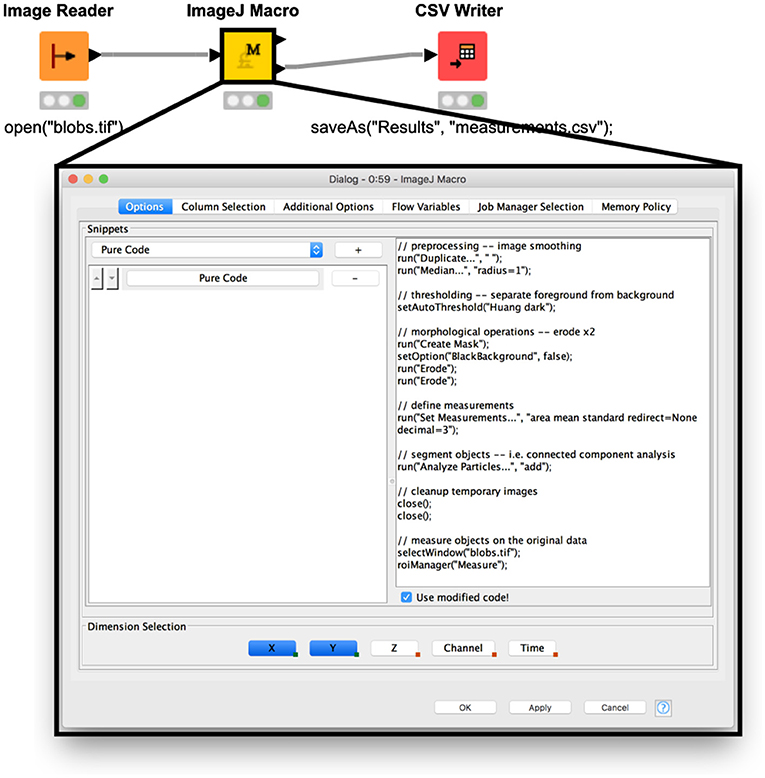
Figure 1. An ImageJ Macro node performing image segmentation and feature extraction.

Nodes of the KNIME Image Processing Extension

The KNIME Image Processing extension includes many nodes for image processing tasks that can be used to invoke image processing functionality driven by ImageJ. From a user's perspective, this means that they are using ImageJ libraries “under the hood” without requiring explicit knowledge of technical details.

For guidance on building image analysis pipelines using the KNIME Image Processing extension, we refer the reader to the previously published KNIME Image Processing tutorial (Dietz and Berthold, 2016), as well as in A Blueprint for Image Segmentation Using ImageJ and KNIME Analytics Platform below, which presents a blueprint for converting an ImageJ macro into a full-fledged KNIME workflow.

Wrapping ImageJ Commands as KNIME Nodes

By installing the “KNIME Image Processing—ImageJ Integration” extension (installation instructions at https://www.knime.com/community/imagej), users of the KNIME Analytics Platform gain the ability to use additional ImageJ commands directly as KNIME nodes. Users can install commands in their local KNIME Analytics Platform installations using the KNIME › Image Processing Plugin › ImageJ2 Plugin tab of the File › Preferences dialog, dropping in JAR files containing the commands. Alternately, software developers can make ImageJ commands available via KNIME update sites so that users can instead install them by KNIME's standard mechanism, accessible via File › Install KNIME Extensions… (see https://docs.knime.com/2019-12/analytics_platform_quickstart_guide/#extend-knime-analytics-platform for complete details). An advantage of the latter approach, similar to ImageJ update sites, is that new versions of ImageJ commands can be shipped by developers, freeing individual users of the burden of repeatedly downloading and installing JAR files.

In this way, many ImageJ commands provided and maintained by community members can therefore be treated as fully functional KNIME nodes with no additional work from the maintainers (although to make installation as convenient as possible for KNIME users, it is recommended for developers to publish the commands to a KNIME update site). The autogenerated KNIME nodes automatically support important KNIME node interfaces, particularly streaming and column selection. Any needed configuration of the command is provided through the standard KNIME node configuration dialog. The resulting node can directly be used in conjunction with all other nodes of the KNIME Image Processing extension: input ports are connected to an image source, output ports provide the processed results, and no scripting or programming experience is required.

In addition, developers can code algorithms that run in both KNIME Analytics Platform and ImageJ without requiring a deeper knowledge of the KNIME application programming interface (API); only a basic knowledge of how to write an ImageJ command is required (https://imagej.net/Writing_plugins).

Figure 2 shows an example workflow (https://kni.me/w/DU4eH3TjYhcxfWXD) utilizing a low-pass filter from the ImageJ tutorials (https://github.com/imagej/tutorials) exposed as a KNIME node and executed on one of ImageJ's sample images (https://imagej.net/images/lymp.tif). To reproduce this workflow, follow the instructions in the workflow description on KNIME Hub. The command's ImageJ menu path (Tutorials › Low-Pass Filter) defines the node's placement within the Node Repository. The filter utilizes forward and backward fast Fourier transforms, available as part of the ImageJ Ops library, but not yet wrapped as built-in KNIME Image Processing nodes.

FIGURE 2

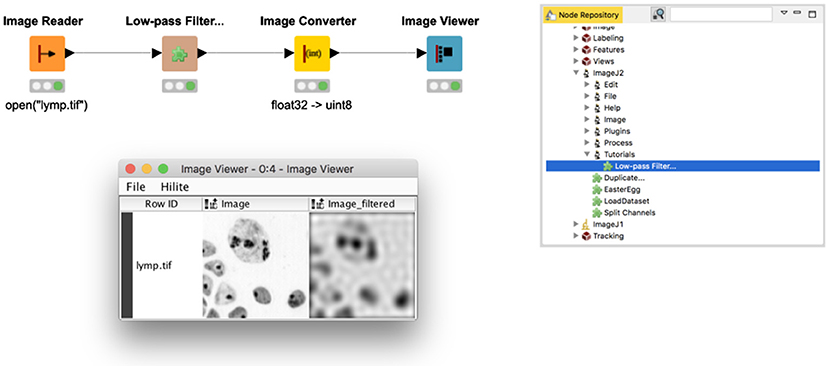
Figure 2. An ImageJ command for low-pass filtering used as a KNIME node.

Embedding Custom Java Code

Advanced users can apply the Java Snippet node (https://kni.me/n/QNB4FsAPnEAgOMVh) to run custom Java code directly without needing to package it as an ImageJ command. Such code snippets have many more applications than only image processing, offering direct access to KNIME data structures, with great flexibility in the input and output types they can be configured to use, as well as the ability to depend on additional libraries present in the environment. Because the KNIME Image Processing extension includes ImageJ's underlying libraries, Java Snippet nodes can, in combination, readily exploit these libraries to perform custom image processing routines.

Figure 3 illustrates usage of a Java Snippet node to clear the image area outside a defined spherical region of interest (ROI). The workflow (available on the KNIME Hub at https://kni.me/w/ThmsDDG4kj-_Ecml) first generates random image data for demonstration purposes. The Java snippet code then makes a copy of the input image and iterates over its samples, checking whether each sample lies within the sphere and, if not, setting its value to zero.

FIGURE 3

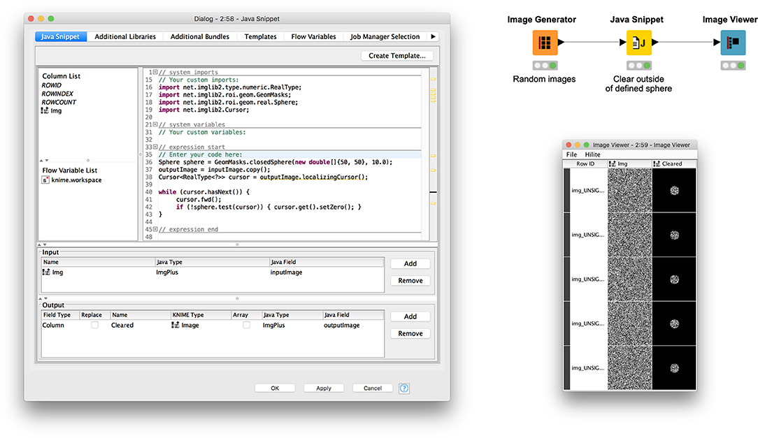
Figure 3. An example Java Snippet node operating on an image region of interest using ImgLib2 libraries.

For more information on how to implement image processing algorithms with ImgLib2, see the ImageJ developer documentation (https://imagej.net/Development).

Noteworthy ImageJ Pitfalls

ImageJ has some historical idiosyncrasies worth mentioning here, which might surprise or confuse users seeking to emulate classical ImageJ operations within the KNIME Analytics Platform.

The behavior of ImageJ's binary operations varies depending on several factors: (1) color lookup tables (LUTs) used for visualization can be inverted (Image › Lookup Tables › Invert LUT); (2) the Image › Adjust › Threshold dialog has a “Dark background” checkbox inverting the thresholded range; and (3) the Process › Binary › Options… menu has a “Black background” toggle that inverts how binary operations perform on masks and how masks are created from thresholded images. The interaction between these three factors can be confusing:

• For an image with a normal LUT, “Dark background” selects higher-intensity values as foreground. But if the LUT is inverted, “Dark background” selects lower-intensity values as foreground.

• When creating a mask (Edit › Selection › Create Mask) from a thresholded image, the mask will be 8-bit type with 255 values for foreground and 0 values for background. But if the “Black background” option is off, an inverted LUT will be used such that foreground values appear black while background values appear white.

• Furthermore, binary morphological operations such as erosion (Process › Binary › Erode) operate on the appearance rather than the intensity value of the mask. For example, a mask with inverted LUT has 255 values that appear black; but when the “Black background” option is set, these 255 values are considered to be background, and the Erode command grows the 255 values at the boundary, rather than reducing them—whereas the same mask with non-inverted grayscale LUT will have those same 255 values appearing white and thus considered to be foreground, with Erode reducing them at the boundary.

The redesigned version of ImageJ (Rueden et al., 2017, p. 2) dispenses with the concept of inverted LUTs and includes a dedicated 1-bit image type for masks, where 0 always means background and 1 always means foreground. The KNIME Image Processing nodes and ImageJ integration are built on the new ImageJ and inherit these design choices. However, users migrating ImageJ workflows that include binary morphological operations are advised to be careful: if the ImageJ workflow assumes the “Black background” option is off, or if inverted LUTs are used, the behavior in the KNIME Analytics Platform will be reversed compared to ImageJ.

Another notable idiosyncratic behavior of ImageJ is that of ImageJ's rank filters such as the median filter (Process › Filters › Median…). The behavior of these filters in the new ImageJ—and hence also the KNIME Image Processing nodes—has been brought in line with other image processing routines. While ImageJ's built-in rank filters are limited to circular masks for computing filter responses, KNIME Image Processing nodes support rectangular masks as well. In addition, this choice of mask is made explicit by exposing the setting in the configuration dialog instead of implying a convention through the Process › Filters › Show Circular Mask… command. Running this command in ImageJ reveals that additional circular masks with non-integer radii, e.g., 0.5, 1.5, etc., are available: those radii change the discretization of the circular mask on the pixel grid. By supporting integer radii only, KNIME Image Processing follows the convention of other image processing libraries.

The above discussion does not comprise an exhaustive list of differences between ImageJ and KNIME Analytics Platform, but we hope the aforementioned examples raise the reader's awareness of implicit assumptions and the resulting need to compare outputs of different tools for the same operation with the same settings.

A Blueprint for Image Segmentation Using ImageJ and KNIME Analytics Platform

Here, we describe a process for translating ImageJ scripts into KNIME workflows. While bioimage analysis pipelines are, in most cases, developed for specific use cases, they typically share a common scaffold of preprocessing, segmentation, and feature extraction. Hence, for demonstration purposes, we highlight a minimal script in ImageJ's macro language that performs simple actions along these lines (Figure 4, left panel) and corresponding KNIME workflow (Figure 4, right panel). The KNIME workflow can also be found on the KNIME Hub (https://kni.me/w/oZteZanXoWURLouy). Each step of the script has equivalent functionality in KNIME node form as follows:

FIGURE 4

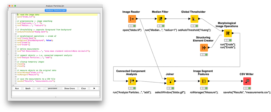
Figure 4. Side-by-side comparison of ImageJ macro with KNIME workflow using KNIME Image Processing nodes.

Open the Image

We are applying the script to ImageJ's well-known “Blobs” example image, accessible from within the ImageJ application via File › Open Samples › Blobs (25K) and often used for demonstration purposes. To open an image in KNIME, we use the Image Reader node (https://kni.me/n/PQRHqpYEOx-QXrbp), which supports reading many scientific image file formats via the SCIFIO and Bio-Formats libraries.

Preprocess the Image

Next, we smooth the image using a median filter. Such preprocessing often helps to achieve a better separation of foreground and background, smoothing away outlying sample values. Neighborhood operations, such as median, require specifying the size and shape of the neighborhood as a “structuring element.” ImageJ's Process › Median… command, called from the macro here, will implicitly use a rectangular neighborhood with radius 1 (i.e., a 3 × 3 square). In the corresponding Median Filter node (https://kni.me/n/OPevaIVf-GfJ1NXJ), we specify the same neighborhood by setting a Span of 1 and Neighborhood Type of RECTANGULAR.

Threshold the Image

Subsequently, an automated global thresholding algorithm (Huang and Wang, 1995) is applied to generate a binary mask of foreground (i.e., areas with objects of interest) vs. background (i.e., areas without such objects) pixels. In ImageJ, the command is Image › Adjust › Threshold…; in KNIME Image Processing, the node is Global Thresholder (https://kni.me/n/L0bv0drXtgAsdbFe). Both of these support the same thresholding methods.

Adjust the Mask

In some scenarios, the thresholded mask may either over- or underrepresent the foreground. For example, in cell biology, the mask might include cell membranes when measuring only cell interiors is desired. Morphological operations such as erosion—shrinking the foreground along its border—or dilation—likewise expanding the foreground—can be used to adjust the mask to minimize this issue so that objects can be measured as accurately as possible. In ImageJ, these morphological operations are found in the Process › Binary submenu; the corresponding KNIME Image Processing functionality is the Morphological Image Operations node (https://kni.me/n/NriZ1-GeHMqitd1c), with an assist from the Structuring Element Creator (https://kni.me/n/AePOcxewSCvaUiZh) node. In this example, we reduce the size of the objects by applying a 2-pixel erosion using a rectangular (as opposed to spherical) structuring element.

Divide the Mask Into Objects

Now that the mask has been optimized, we can perform a connected component analysis to split the mask foreground into individual objects. In ImageJ, the Analyze › Analyze Particles… command is often used to accomplish this, although it also can bundle in other steps, such as object measurement. In our case, we do not want to measure image features yet because it would measure the image mask rather than the original image data. Thus, we simply split up the foreground into ROIs and add each ROI to ImageJ's ROI Manager, with the intent of measuring them in a later step. In KNIME terms, the Connected Component Analysis node (https://kni.me/n/aFTAPO7mEW_Okby7) does exactly what we want, which is to convert the binary mask into an image labeling, with each label corresponding to a distinct object.

Measure Object Features on Original Image Data

With the image divided into objects, we can now measure each object. We are interested in both spatial features—relating to the shape of the object—and image features—related to the object's content (i.e., its sample values). From ImageJ's ROI Manager, clicking the Measure button generates a Results window with a table of measurements, one row per object, one column per measurement. Which features are computed is configurable globally via the Analyze › Set Measurements… dialog. In our example, we compute area, mean value, and standard deviation. In the equivalent KNIME workflow, we use the Image Segment Features node to compute the same features: on the Features tab, under “First order statistics,” we select Mean and Std Dev, and under “Segment geometry,” we select Num Pix. However, this node requires as input a combined table including both the original image data in one column and corresponding image labeling in another column. The Joiner node enables us to create this combined table, which we then feed into Image Segment Features; a new table of measurements, analogous to ImageJ's Results table, is then produced.

Export Resulting Measurements

Finally, the Results table is exported to a CSV file on disk, which can subsequently be imported into other programs—e.g., a spreadsheet application or R script—for further analysis, figure generation, and so forth. In ImageJ, with the Results window active, the File › Save As … command is used to create the CSV file. The corresponding KNIME node is CSV Writer. However, it is worth noting that with KNIME workflows, it is often not necessary to export data for further analysis in an external tool because there are KNIME nodes for manipulating and analyzing tabular data (see, e.g., Analytics nodes in Node Repository view), integrating with other powerful platforms such as R (https://kni.me/e/6cbZ6X3DrLrH96WD) and Python (https://kni.me/e/9Z2SYIHDiATP4xQK), and generating figures (see, e.g., Views nodes in Node Repository view).

Biological Use Cases

The nature of individual KNIME nodes naturally lends workflow development to compartmentalize functionality. This is facilitated by creating components that enclose multiple, discrete nodes. Not only does this facilitate development by allowing the designer to optimize individual functionality and test discrete functionalities, but it also enables portability of discrete functions. The following use cases leverage this compartmentalization to facilitate their deployment.

Biological Use Case No. 1: Quantitative Analysis of Subcellular Structures

The goal of this analysis was to quantitatively assess the ability of a cytoskeletal organizer to control adhesion to the extracellular matrix. In this case, adhesion is visualized by the formation of focal adhesion complexes. A quantitative comparison was achieved by extrapolating the number of focal adhesion complexes formed at the periphery of the cell vs. within the center of the cell. The KNIME workflow (Figure 5) was divided into five sequential steps with discrete objectives: (1) reading of file in, (2) processing of the images into labels that capture the individual focal adhesion complexes, (3) arithmetic on the labels to obtain the characteristics (features) for classification, (4) classification of the labels using extracted features, and (5) visualization of the classified focal adhesion complexes (periphery vs. center).

FIGURE 5

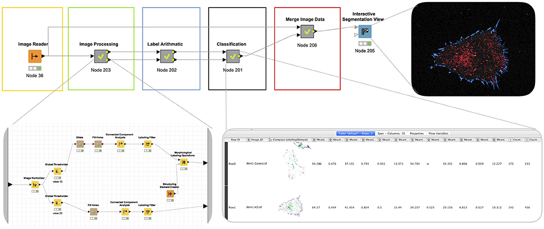
Figure 5. Quantitative analysis of subcellular structures. To analyze the consequences of disrupting the cytoskeleton on matrix adhesion focal adhesion complex formation is visualized using total internal reflection fluorescence (TIRF) imaging. A KNIME workflow was leveraged to define the number of focal adhesion complexes at the periphery of the cell vs. within the center of the cell using sequential steps with discrete objectives: (I) Read file in, (II) processing of the images into labels that capture the individual focal adhesion complexes, (III) arithmetic on the labels to obtain the characteristics (features) for classification, (IV) classification of the labels using extracted features, and (V) visualization of the classified focal adhesion complexes (periphery vs. center). Note that the output of this pipeline is a combination of visualization and quantitation. Both of these can be leveraged for further analysis.

Image data for extrapolating the full cell body and the individual focal adhesion complexes were remarkably similar. Both aspects of the pipeline were extracted from the same normalized images, which were thresholded manually (Global Thresholder node) and then processed by the Connected Component Analysis node to generate image segments for either the full cell body or individual focal adhesions. To select the pixels for the full cell body, the threshold was set lower (10), and the combination of Dilate and Fill Holes was used to ensure a full inclusion of the cell body. For the selection of the focal adhesions, the threshold was set higher (25), and image dilation was omitted to enable a narrow selection of image segments reflecting only the focal adhesions. The Label Arithmetic node was subsequently used to define the periphery and the center of the cell. After feature extraction, the peripheral and central focal adhesion complexes were defined by their relative proximity within the cell (Classification). These classified focal adhesion were then mapped back to the original images.

Compartmentalization of the sequential functions facilitated optimization of the image processing functions. Once discrete focal adhesion complexes were defined, these objects were readily transformed to labels that could be quantitatively interrogated, both for their location as well as their intrinsic features (i.e., size, shape, etc.). The output of these data types was readily joined and visualized by overlaying the labels for peripheral and central focal adhesion complexes back to the original image.

Biological Use Case No. 2: Quantitative Analysis of a Histological Stain

The goal of this analysis was to generate an objective and quantitative measure of the chromogenic tissue stain via the histological staining of a cell adhesion marker related to tumor invasion and metastasis, demonstrating significant variation across patient samples. As in the previous use case, the KNIME workflow (Figure 6) was divided into sequential steps that complete discrete objectives: (1) reading of file in; (2) preprocessing of the images and their annotation in preparation for analysis using ImageJ functionalities; (3) pixel classification using Weka-based machine learning functionality; (4) post-classification processing of image data to labels that correspond to positive; (5) compilation of labels, images, and annotations; and (6) visualization of the quantitation by overlaying the labels with the original image. Unlike the first use case, the objects of interest could not be generated using conventional thresholding. Instead, a trainable segmentation strategy was employed to generate a pixel classification model. While this approach is much more resource intensive, it was effective in defining objects in complex images. The label processing and visualization was very similar to the first use case. While it was not deployed here, the labels created in this workflow could easily be used to perform quantitative analysis of the stain within the tissue.

FIGURE 6

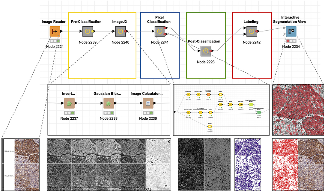
Figure 6. Quantitative analysis of histological stain. The histological staining of a cell adhesion marker (CD166) related to tumor invasion and metastasis demonstrates significant variation across patient samples. As in user case no. 1, the KNIME workflow was divided into sequential steps that complete discrete objectives: (1) read in file, (2) preprocessing of the images and their annotation in preparation for analysis using ImageJ2 functionalities, (3) pixel classification using Weka-bases machine learning functionality, (4) post-classification processing of image data to labels that correspond to “positive,” (5) compilation of labels, images, and annotations, (6) visualization of the quantitation by overlaying the labels with the original image.

ImageJ elements were implemented in multiple steps. After splitting the channels with Splitter “Pre-classification,” a target image (for pixel classification) was generated through sequential processing with Invert, Gaussian Blur, and Image Calculator, with the goal of eliminating background pixel values not relevant to the tissue stain. Pixel classification was subsequently achieved using the Fiji Trainable Segmentation Features 2D. The selected pixels were transformed to labels using Connected Component Analysis after eroding the pixel segments with Erode to facilitate separation of individually stained areas. Finally, the labels corresponding to the stain was joined with original image data and visualized using the Interactive Segmentation Viewer.

Note that this workflow could be significantly simplified if the original data had been acquired as a multilayer TIFF or if the project had been completed with a monocolor fluorescent stain rather than a chromogenic stain. However, we often do not have control over the original data acquisition, thus highlighting the need for flexibility and creativity in our data analysis approach.

Biological Use Case No. 3: Channel-Shift Correction and Particle Tracking

This KNIME workflow (Figure 7) corrects particle-tracking data coming from a three-camera system that was used to acquire live-cell time-lapse series of genomic loci labeled with three different fluorescent markers. The distance between two differently labeled loci in a cell nucleus can be in the range of a few hundred nanometers, and it is crucial to determine these distances as accurately as possible, within the physical and optical limits of the experimental system, to test hypotheses about chromosome conformation and dynamics (Tiana et al., 2016). This requires correcting for possible rotations and misalignments between cameras, as well as for chromatic aberrations specific to each color channel.

FIGURE 7

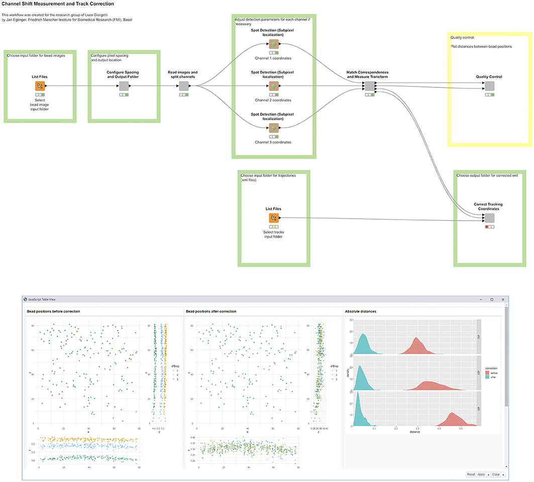
Figure 7. A KNIME workflow for channel-shift correction and particle tracking. The positions of bead detections are shown in three-pane scatter plots, before (left) and after (right) applying channel-shift correction. The density plots show absolute distances between apparent bead locations of two channels (red) and after (cyan) correction.

To measure the channel shift and chromatic aberration, autofluorescent beads were imaged with acquisition settings corresponding to those used in live-cell imaging. In the acquired image stacks, the bead locations were determined at subpixel accuracy using a spot detection algorithm provided by the ImageJ plugin, TrackMate (Tinevez et al., 2017), and the ImgLib2 (Pietzsch et al., 2012, 2) library in Fiji. Subsequently, the channels were registered by aligning these bead locations, using the ImageJ plugin, “Descriptor-based registration” (Preibisch et al., 2010), and the library, “mpicbg;” both are included in Fiji (Schindelin et al., 2012). We implemented all functionality as ImageJ/SciJava command plugins (https://github.com/fmi-faim/fmi-ij2-plugins/) that give rise to autogenerated KNIME nodes. To assess the quality of the correction and aid in choosing a suitable transformation model, we plotted the distances between corresponding bead positions in the different channels before and after correction, using the R scripting integration in KNIME. The deviations between apparent bead locations in different channels provide an estimate of the overall particle localization accuracy in the experiment, which was below 50 nm after correction. The measured transformation for each channel was then used to correct point coordinates derived from tracking labeled genomic loci in live-cell imaging data.

In this use case, according to the strengths of the respective software packages, tracking was performed interactively with TrackMate in ImageJ (i.e., outside KNIME), while the KNIME workflow was used to automate correction of coordinates in the TrackMate results files (in XML format). Instead of correcting coordinates, it is also possible to apply the measured transformation to images for downstream processing. However, as this would involve significantly more computation, we chose to work on the coordinates in this case.

Biological Use Case No. 4: Single-Cell Analysis in Prostate Cancer

Androgen receptor (AR) is a critical protein in the progression of prostate cancer and benign prostate diseases. The activity of AR protein is defined by the activation of target genes such as PSA or AR presence in the nucleus (Wang et al., 2002). Consequently, treatments for prostate cancer are focused on targeting the AR pathway and preventing AR translocation to the nucleus (Higano and Crawford, 2011). Assessing AR localization and activity in response to ligands or drugs normally requires manual nucleus and cytoplasm segmentation. Achieving sufficient data points to determine if an observed phenotype occurs with a given confidence renders manual image segmentation difficult. These limitations inspired us to develop an automated image segmentation and analysis workflow via the KNIME platform in conjunction with ImageJ plugins.

Briefly, our image processing workflow accepts multichannel images (.TIF and .ND2) and requires a nuclear marker/stain in the first channel, with the subsequent channels arranged as desired. First, cells are identified via the nuclear channel by a series of ImageJ plugins that perform image and illumination correction. The data are then passed to the Global Thresholder node (default: Otsu method) to threshold the nuclear signal, Morphological Image Operations node to dilate nuclear signal (i.e., dilate the threshold mask), the Fill Holes node to create a smooth nuclear mask, and finally, the Waehlby Cell Clump Splitter node to separate closely clustered nuclei. The nuclear masks generated by our workflow are then dilated with the Morphological Image Operations node to create a nuclear mask larger than the original. To create the cytoplasmic measurement mask—here referred to as the “cytoplasmic ring”—the larger, dilated nuclear masks and the original smaller nuclear masks are next processed by the Voronoi Segmentation node to produce a ring-shaped mask located in the cytoplasm of a tracked cell. Simultaneously, the other channels are processed through ImageJ macro nodes to subtract the background before obtaining measurements for the nuclear and cytoplasmic compartments. In the final step, the nuclear and cytoplasmic masks are applied to the non-nuclear channels (i.e., the measurement channels) to measure the signal in the nuclear and cytoplasmic compartments, respectively.

In this experiment, we tested AR-positive LNCaP cells with the potent synthetic AR ligand R1881, which induces AR translocation to the nucleus (Figure 8A). Using KNIME and the image processing workflow that we developed, we were able to measure this cytoplasmic-to-nuclear translocation over hundreds of cells. Plotting these data in an xy scatter plot (Figures 8B, C) reveals the nuclear translocation of AR in response to the R1881 synthetic ligand. This software will allow us to test future therapeutic agents targeting the AR pathway and AR activation in benign prostate diseases and prostate cancer.

FIGURE 8

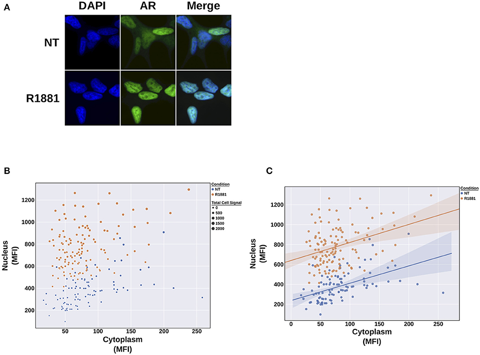
Figure 8. R1881 treatment shows nuclear translocation of the androgen receptor in LNCaP cells. (A) LNCaP cells were either left non-treated or treated with 1 nM R1881. Under R1881 treatment conditions, androgen receptor (AR) localization shifts from nuclear and cytoplasmic to primarily nuclear. (B) xy scatter plot of the mean fluorescence intensity (MFI) of the cytoplasm (x) and the nucleus (y). The size of the point denotes sum of the cytoplasmic and nuclear signal (i.e., total cell signal). Treating LNCaP cells with R1881 induces a shift into the nucleus and increase in signal inside the nucleus. (C) a linear regression plot depicting the clear separation of the populations.

Materials and Methods

KNIME ImageJ Integration

The KNIME Image Processing extension is built on the same technologies that have driven the latest versions of ImageJ, including ImgLib2, a general-purpose, multidimensional image processing library (Pietzsch et al., 2012); SCIFIO, a framework for reading and writing scientific image formats (Hiner et al., 2016); Bio-Formats, a Java library for reading and writing life sciences image file formats (Linkert et al., 2010); and BigDataViewer (Pietzsch et al., 2015), a reslicing browser for terabyte-sized multiview image sequences. This infrastructure enables code reuse across tools beyond KNIME and ImageJ, facilitating consistency across a broader range of software incorporating the same underlying algorithms. This technology selection allows KNIME and ImageJ to directly share data, avoiding costly data serialization operations. ImageJ routines are called in-process, in contrast to many interprocess integrations, especially cross-language ones, which require duplicating data at the expense of additional computation time and disk space.

The KNIME Image Processing extension (https://kni.me/e/Uq6QE1IQIqG4q_mp) can be found on the “Community Extension (trusted)” update site. KNIME Image Processing–ImageJ Integration extension (https://kni.me/e/jwXXJ1i4i6fknco2) is part of Community Extension (experimental). Detailed installation instructions can be found in the Extension and Integration Guide (https://docs.knime.com/2019-06/analytics_platform_extensions_and_integrations/). The KNIME Image Processing extension source code can be found on GitHub (https://github.com/knime-ip/knip, https://github.com/knime-ip/knip-imagej2).

Depending on the needs of the developer, several possibilities exist for extending the KNIME Analytics Platform with additional functionality based on the KNIME Image Processing ecosystem. The most flexible approach is to write a native KNIME node (see https://www.knime.com/blog/the-five-steps-to-writing-your-own-knime-extension). For ImageJ-related extensions, the simpler mechanism of writing an ImageJ command plugin and wrapping it as a KNIME node is a powerful option—see A Blueprint for Image Segmentation Using ImageJ and KNIME Analytics Platform; and Wrapping ImageJ Commands. However, autogeneration of KNIME nodes from ImageJ commands requires them to conform to certain input and output parameter types: not all ImageJ plugins can currently be executed with KNIME. Furthermore, the ImageJ command must declare itself to support headless operation via the headless=true parameter to ensure compatibility with KNIME's “configure once, execute often” paradigm. An example implementation of an ImageJ2 command can be found at https://github.com/knime-ip/knip-imagej2/tree/0.11.6/org.knime.knip.imagej2.buddydemo/src/org/knime/knip/imagej2/buddydemo. For further details, please see https://www.knime.com/community/imagej.

Biological Use Cases

Biological Use Case No. 1: Detection of Subcellular Structures

Focal adhesion complexes were visualized through total internal reflection fluorescence (TIRF) confocal microscopy with a Nikon Multi-Excitation TIRF using Apo TIRF 60 × /1.49 objective using 0.7-s frame capture on a Andor Xyla sCMOS after 488 nm diode laser excitation in single TIRF mode. Fluorescent-labeled vinculin is localized to the contact point between the cell and the surface below. Tiff files were exported from the Nikon Elements software for further processing. After image normalization, two parallel tracks were used to generate separate labels for the focal adhesion complexes, the periphery of the cell, and the center of the cell. Label arithmetic was subsequently used to delineate which focal adhesion complexes were at the center and which were in the periphery. The KNIME workflow is available on KNIME Hub (https://kni.me/w/7yXlo4oq91qSBWeU); image data is published on Figshare (https://doi.org/10.6084/m9.figshare.9936281.v2).

Biological Use Case No. 2: Histological Detection of CD166 in Tissue Sections

Formalin-fixed, paraffin-embedded bladder tumors were sectioned (6 μm) and processed for immunostaining as described previously (Hansen et al., 2013; Arnold et al., 2017). Briefly, the cell surface adhesion molecule was detected within the tissue using conventional 3,3' diaminobenzidine (DAB; brown) staining. The tissue was counterstained using hematoxylin (blue nuclear stain). Images were captured with the Leica SCN400 Slide Scanner using a HC PLAN APO 20 × /0.7 (dry) objective into.scn tiled file format. Image tiles (1,000 × 1,000 pixels) were extracted using Aperio Imagescope and saved in JPEG2000 format. The areas of the tissue that contain DAB stain were identified through a trainable pixel classification scheme. To achieve this, the image is split into its three individual channels and processed with a series of ImageJ functions to generate an image that reflects the DAB pixel values after subtraction of background signal from the other three channels. In the pixel classification node, the data are split into a training and test set. Using the interactive annotator, labels annotating the pixels of interest are created, while pixel features are extracted in a parallel. The selected pixel features are used to train a model, which is subsequently applied to both training and test images. Selected pixels are subsequently transformed to a label, which is mapped back to the original images to visualize positive areas. The KNIME workflow and datasets are available on KNIME Hub (https://kni.me/w/QVjrs0Vj7xG48Pcr). Before opening this workflow, you need to add the nightly software site to your KNIME installation (see https://knime.com/wiki/knime-image-processing-nightly-build for details). Once the site is enabled, upon opening the workflow, KNIME will search for the required extension and install it automatically.

This study was carried out in accordance with the recommendations of the Vanderbilt Institutional Review Board (IRB). The protocol was approved by the IRB under protocol no. 150278 “Assessment of cell migration in cancer.” Where necessary, all subjects gave written informed consent in accordance with the Declaration of Helsinki.

Biological Use Case No. 3: Channel-Shift Correction and Particle Tracking

For chromatic shift correction, autofluorescent beads were acquired using the VisiView software (Visitron) on a Nikon Eclipse Ti-E inverted microscope equipped with a CFI APO TIRF 100×/1.49 oil objective lens (Nikon) and three Evolve 512 Delta EMCCD cameras (Photometrics). For live-cell tracking of genomic loci, cell lines were prepared as described earlier (Masui et al., 2011; Tiana et al., 2016) and imaged at a frame interval of 30 s.

The KNIME workflow is available on KNIME Hub (https://kni.me/w/F3K1YgZKt_923UgH); image data are included with the workflow. The ImageJ command plugins (see Wrapping ImageJ Commands as KNIME Nodes) used in this analysis are wrapped in the FMI KNIME Plugins extension, which is provided by the FMI KNIME Plugins update site (https://community.knime.org/download/ch.fmi.knime.plugins.update): this extension must be installed via the File ffl Install KNIME Extensions… dialog before executing the workflow. The workflow consists of several steps (Figure 7): (1) configuration (file input and output locations, metadata), (2) image reading and channel splitting, (3) configurable spot detection, (4) spot matching and transformation measurement, (5) quality control (distance measurement and plotting), and (6) applying the correction onto tracking data.

Biological Use Case No. 4: Single-Cell Analysis in Prostate Cancer

Immunofluorescence (IF) was performed on LNCaP cells using Cell Signaling Technology's protocol (Abcam, Cambridge, United Kingdom). Cells were fixed in 4% paraformaldehyde, permeabilized, and washed. Cells were then incubated with the primary antibody AR (1:600, Cell Signaling Technology; Cat. No. 5365) at 4°C overnight. The next day, this was followed by antirabbit conjugated to AlexaFluor 488 (Thermo Fisher Scientific, Cat. No. A-21206). DAPI was used as a nuclear counterstain at 1:250. fluorescein isothiocyanate (FITC) (500 ms) and DAPI (125 ms) channels were then acquired using a Nikon Eclipse 80i microscope with a Retiga 2000R at 40× magnification. Subsequent data—available via Figshare (https://doi.org/10.6084/m9.figshare.9934205.v1)—were then analyzed using the KNIME workflow available on the KNIME Hub (https://kni.me/w/QMky8ZEz3dzja42q). This study was carried out in accordance with biosafety protocol B00000511 approved by the University of Wisconsin-Madison Institutional Biosafety Committee.

Discussion

The KNIME Image Processing extension with its ImageJ integration offers many benefits in interoperability, efficiency, and functionality when deployed to solve bioimage analysis problems. Ideally, the decision to use the KNIME Analytics Platform will not limit the user to just one software solution but, quite the contrary, open up the possibility to combine a wide array of other integrated tools and software to achieve the best result. The goal of the KNIME Analytics Platform is to provide a common foundation from which users and developers alike can explore and utilize a wide ecosystem of analysis tools. This approach leads to better image analysis outcomes while also enabling new combinations of functionality that would not be feasible otherwise.

Not only does an open, extensible, and integrated platform enable users to benefit from readily available tools, it also empowers developers to further enhance the platform with their own reusable algorithms and tools. The ImageJ and KNIME Image Processing teams together are continuing to work on making it even easier for researchers to integrate custom functionalities across an array of open-source platforms, including ImageJ scripting and ImageJ Ops (Table 1). Future directions include the following.

TABLE 1

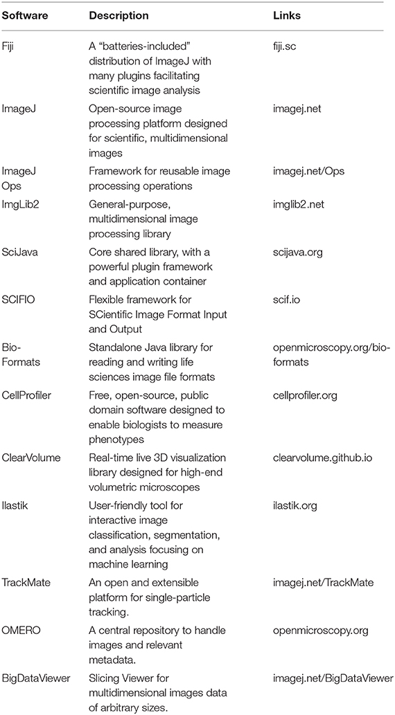
Table 1. Representative integrated tools and libraries related to bioimage data analysis.

Facilitating Deployment

One of the most important factors of ImageJ's success is its easy extensibility and sharing of custom code with other researchers, leading to a great wealth of plugins for many tasks. Most available plugins are distributed to users via so-called update sites, either hosted individually or by ImageJ itself. Although the KNIME Analytics Platform also includes a robust update site mechanism, it imposes a higher technical barrier than ImageJ does. Hence, in the future, we want to make it easier to share and install ImageJ plugins as KNIME nodes for developers with even less technical backgrounds and training.

Large Image Support

The KNIME Image Processing extension's core infrastructure will also be improved to handle new types of image data. For instance, advances in microscope technology in the last few years have not only lead to an increase in the amount of image datasets but also a substantial increase in the size of single images. Multiview light-sheet microscopy (Huisken and Stainier, 2009), for example, allows researchers to create (nearly) isotropic three-dimensional volumes over time, which easily comprise hundreds of gigabytes. This relatively new modality of images requires the development of not only new tools to visualize and explore the data but also architectures to efficiently process the data (Preibisch et al., 2010, 2014; Schmid and Huisken, 2015). Therefore, our future work includes the integration of tools for processing extremely large images, for example through use of cacheable, block-based ImgLib2 images (https://github.com/imglib/imglib2-cache) as the KNIME Image Processing extension's primary data structure.

Scripting

One of the most critical features for users of ImageJ is the capability to record and write scripts in various supported scripting languages such as JavaScript, Groovy, Jython, and ImageJ's own macro language (https://imagej.net/Scripting). Such scripts enable ImageJ users to define workflow-like behavior via sequential execution of ImageJ functions. A future version of KNIME ImageJ integration will add the ability to create full-fledged KNIME nodes via ImageJ scripting. Similar to the automatic node generation from ImageJ command plugins (see Wrapping ImageJ Commands as KNIME Nodes), these scripts will automatically become nodes seamlessly integrated into the KNIME Analytics Platform.

Accessing ImageJ functionality via the KNIME Analytics Platform not only enhances the interoperability of different existing bioimaging applications but also directly inherits further advantages, including improved reproducibility and documentation of results, a common and user-friendly graphical user interface, and the ability to process large amounts of image data, potentially combining with data from entirely different domains. These powerful integrations and the other aforementioned advantages make the KNIME Analytics Platform an effective gateway for ImageJ users to create both simple and complex workflows for biological image data analysis, empowering scientists of various backgrounds with state-of-the-art methods and tools to propel science forward together.

Data Availability Statement

KNIME Analytics Platform and the KNIME Image Processing extension are free/libre open source software (FLOSS) licensed under the GNU General Public License (GPL) (https://www.knime.com/downloads/full-license), with source code available on Bitbucket (https://bitbucket.org/KNIME/) and GitHub (https://github.com/knime-ip/), respectively. ImageJ and its supporting libraries are open-source software collections with permissive licensing (https://imagej.net/Licensing). All KNIME workflows presented in this paper are published to the KNIME Hub (https://hub.knime.com/) with links inline in the body of the article. Corresponding datasets for KNIME workflows for biological use cases 1, 2, and 4 can be found via Figshare (https://doi.org/10.6084/m9.figshare.c.4687004.v1). Corresponding datasets for biological use case #3 are available via KNIME Hub (https://kni.me/w/F3K1YgZKt_923UgH).

Ethics Statement

This study was carried out in accordance with the recommendations of the Vanderbilt Institutional Review Board (IRB). The protocol was approved by the IRB under protocol #150278 Assessment of cell migration in cancer. Where necessary, all subjects gave written informed consent in accordance with the Declaration of Helsinki.

Author Contributions

CD, CR, MB, and KE conceptualized and designed the study. CD, CR, and MH did the primary code development presented with support from SH and ED on KNIME and ImageJ use cases, respectively. JE, EE, DM, WR, NS, and AZ contributed to the experiments and to descriptions in the paper. All authors contributed to the manuscript text.

Funding

We acknowledge funding from the Chair for Bioinformatics and Information Mining (MB), German Network for Bioinformatics (de.NBI) grant number no. 031A535C (MB), the Morgridge Institute for Research (KE), Chan Zuckerberg Initiative (CR and KE), NIH U54 DK104310 (WR), NIH R01 AI110221 (NS), NIH R01 CA218526 (AZ), and NIH RC2 GM092519-0 (KE). We also acknowledge NIH T32 CA009135 (EE) and a Science & Medicine Graduate Research Scholars Fellowship through the University of Wisconsin-Madison (EE).

Conflict of Interest

CD, SH, and MB have a financial interest in KNIME GmbH, the company developing and supporting KNIME Analytics Platform.

The remaining authors declare that the research was conducted in the absence of any commercial or financial relationships that could be construed as a potential conflict of interest.

Acknowledgments

The authors are grateful for code contributions and design discussions from many software developers including (in alphabetical order): Tim-Oliver Buchholz, Barry DeZonia, Gabriel Einsdorf, Andreas Graumann, Jonathan Hale, Florian Jug, Adrian Nembach, Tobias Pietzsch, Johannes Schindelin, Simon Schmid, Daniel Seebacher, Marcel Wiedenmann, Benjamin Wilhelm, and Michael Zinsmaier. We furthermore acknowledge the strong support of the software communities covered in this manuscript, in particular the developers and users of the KNIME Analytics Platform, ImgLib2, ImageJ, and Fiji. For biological use case no. 1, we thank Katie Hebron for providing the images. For biological use case no. 3, we thank Tania Distler, Marco Michalski, and Luca Giorgetti for providing image and tracking data.

References

Afgan, E., Baker, D., van den Beek, M., Bouvier, D., Cech, M., Chilton, J., et al. (2018). The galaxy platform for accessible, reproducible and collaborative biomedical analyses: 2018 update. Nucleic. Acids. Res. 44, W3–W10. doi: 10.1093/nar/gkw343

CrossRef Full Text | Google Scholar

Aiche, S., Sachsenberg, T., Kenar, E., Walzer, M., Wiswedel, B., Kristl, T., et al. (2015). Workflows for automated downstream data analysis and visualization in large-scale computational mass spectrometry. Proteomics 15, 1443–1447. doi: 10.1002/pmic.201400391

PubMed Abstract | CrossRef Full Text | Google Scholar

Allan, C., Burel, J. M., Moore, J., Blackburn, C., Linkert, M., Loynton, S., et al. (2012). OMERO: flexible, model-driven data management for experimental biology. Nat. Methods 9, 245–253. doi: 10.1038/nmeth.1896

PubMed Abstract | CrossRef Full Text | Google Scholar

Arganda-Carreras, I., Kaynig, V., Rueden, C., Eliceiri, K. W., Schindelin, J., Cardona, A., et al. (2017). Trainable weka segmentation: a machine learning tool for microscopy pixel classification. Bioinformatics 33, 2424–2426. doi: 10.1093/bioinformatics/btx180

PubMed Abstract | CrossRef Full Text | Google Scholar

Arnold, E., Shanna, A., Du, L., Loomans, H. A., Starchenko, A., Su, P. F., et al. (2017). Shed urinary ALCAM is an independent prognostic biomarker of three-year overall survival after cystectomy in patients with bladder cancer. Oncotarget 8, 722–741. doi: 10.18632/oncotarget.13546

CrossRef Full Text | Google Scholar

Beisken, S., Meinl, T., Wiswedel, B., de Figueiredo, L. F., Berthold, M., and Steinbeck, C. (2013). KNIME-CDK: workflow-driven cheminformatics. BMC Bioinformatics 14:257. doi: 10.1186/1471-2105-14-257

PubMed Abstract | CrossRef Full Text | Google Scholar

Berthold, M. R., Cebron, N., Dill, F., Gabriel, T. R., Kötter, T., Meinl, T., et al. (2008). “KNIME: the konstanz information miner,” in Data Analysis, Machine Learning and Applications. Studies in Classification, Data Analysis, and Knowledge Organization, eds C. Preisach, H. Burkhardt, L. Schmidt-Thieme, and R. Decker (Berlin; Heidelberg: Springer), 319–326.

Google Scholar

Cardona, A., and Tomancak, P. (2012). Current challenges in open-source bioimage informatics. Nat. Methods 9, 661–665. doi: 10.1038/nmeth.2082

PubMed Abstract | CrossRef Full Text | Google Scholar

Carpenter, A. E., Kamentsky, L., and Eliceiri, K. W. (2012). A call for bioimaging software usability. Nat. Methods 9, 666–670. doi: 10.1038/nmeth.2073

PubMed Abstract | CrossRef Full Text | Google Scholar

Dietz, C., and Berthold, M. R. (2016). KNIME for open-source bioimage analysis: a tutorial. Adv. Anat. Embryol. Cell Biol. 219, 179–197. doi: 10.1007/978-3-319-28549-8_7

PubMed Abstract | CrossRef Full Text | Google Scholar

Döring, A., Weese, D., Rausch, T., and Reinert, K. (2008). SeqAn an efficient, generic C++ library for sequence analysis. BMC Bioinformatics 9:11. doi: 10.1186/1471-2105-9-11

PubMed Abstract | CrossRef Full Text | Google Scholar

Eliceiri, K. W., Berthold, M. R., Goldberg, I. G., Ibáñez, L., Manjunath, B. S., Martone, M. E., et al. (2012). Biological imaging software tools. Nat. Methods 9, 697–710. doi: 10.1038/nmeth.2084

PubMed Abstract | CrossRef Full Text | Google Scholar

Fillbrunn, A., Dietz, C., Pfeuffer, J., Rahn, R., Landrum, G. A., and Berthold, M. R. (2017). KNIME for reproducible cross-domain analysis of life science data. J. Biotechnol. 261, 149–156. doi: 10.1016/j.jbiotec.2017.07.028

PubMed Abstract | CrossRef Full Text | Google Scholar

Gudla, P. R., Nakayama, K., Pegoraro, G., and Misteli, T. (2017). SpotLearn: convolutional neural network for detection of fluorescence in situ hybridization (FISH) signals in high-throughput imaging approaches. Cold Spring Har. Symp. Quant. Biol. 82, 57–70. doi: 10.1101/sqb.2017.82.033761

PubMed Abstract | CrossRef Full Text | Google Scholar

Gunkel, M., Eberle, J. P., and Erfle, H. (2017). “Fluorescence-based high-throughput and targeted image acquisition and analysis for phenotypic screening,” in Light Microscopy: Methods and Protocols, eds Y. Markaki and H. Harz (New York, NY: Springer New York), 269–280.

Google Scholar

Gunkel, M., Flottmann, B., Heilemann, M., Reymann, J., and Erfle, H. (2014). Integrated and correlative high-throughput and super-resolution microscopy. Histochem. Cell Biol. 141, 597–603. doi: 10.1007/s00418-014-1209-y

PubMed Abstract | CrossRef Full Text | Google Scholar

Hansen, A. G., Freeman, T. J., Arnold, S. A., Starchenko, A., Jones-Paris, C. R., Gilger, M. A., et al. (2013). Elevated ALCAM shedding in colorectal cancer correlates with poor patient outcome. Cancer Res. 73, 2955–2964. doi: 10.1158/0008-5472.CAN-12-2052

PubMed Abstract | CrossRef Full Text | Google Scholar

Higano, C. S., and Crawford, E. D. (2011). New and emerging agents for the treatment of castration-resistant prostate cancer. Urol. Oncol. 29, S1–S8. doi: 10.1016/j.urolonc.2011.08.013

PubMed Abstract | CrossRef Full Text | Google Scholar

Hiner, M. C., Rueden, C. T., and Eliceiri, K. W. (2016). SCIFIO: an extensible framework to support scientific image formats. BMC Bioinformatics 17:521. doi: 10.1186/s12859-016-1383-0

PubMed Abstract | CrossRef Full Text | Google Scholar

Huang, L.-K., and Wang, M.-J. J. (1995). Image thresholding by minimizing the measures of fuzziness. Pattern Recognit. 28, 41–51. doi: 10.1016/0031-3203(94)E0043-K

CrossRef Full Text | Google Scholar

Huisken, J., and Stainier, D. Y. (2009). Selective plane illumination microscopy techniques in developmental biology. Development 136, 1963–1975. doi: 10.1242/dev.022426

PubMed Abstract | CrossRef Full Text | Google Scholar

Landrum, G. (2013). Rdkit: Open-Source Cheminformatics Software. Available online at: http://www.rdkit.org

Google Scholar

Linkert, M., Rueden, C. T., Allan, C., Burel, J.-M., Moore, W., Patterson, A., et al. (2010). Metadata matters: access to image data in the real world. J. Cell Biol. 189, 777–782. doi: 10.1083/jcb.201004104

PubMed Abstract | CrossRef Full Text | Google Scholar

Masui, O., Bonnet, I., Le Baccon, P., Brito, I., Pollex, T., Murphy, N., et al. (2011). Live-cell chromosome dynamics and outcome of X chromosome pairing events during ES cell differentiation. Cell 145, 447–458. doi: 10.1016/j.cell.2011.03.032

PubMed Abstract | CrossRef Full Text | Google Scholar

Mazanetz, M. P., Marmon, R. J., Reisser, C. B., and Morao, I. (2012). Drug discovery applications for knime: an open source data mining platform. Curr. Top. Med. Chem. 12, 1965–1979. doi: 10.2174/156802612804910331

PubMed Abstract | CrossRef Full Text | Google Scholar

Pietzsch, T., Preibisch, S., Tomancák, P., and Saalfeld, S. (2012). ImgLib2–generic image processing in Java. Bioinformatics 28, 3009–3011. doi: 10.1093/bioinformatics/bts543

PubMed Abstract | CrossRef Full Text | Google Scholar

Pietzsch, T., Saalfeld, S., Preibisch, S., and Tomancak, P. (2015). BigDataViewer: visualization and processing for large image data sets. Nat. Methods 12, 481–483. doi: 10.1038/nmeth.3392

PubMed Abstract | CrossRef Full Text | Google Scholar

Preibisch, S., Amat, F., Stamataki, E., Sarov, M., Singer, R. H., Myers, E., et al. (2014). Efficient bayesian-based multiview deconvolution. Nat. Methods 11, 645–648. doi: 10.1038/nmeth.2929

PubMed Abstract | CrossRef Full Text | Google Scholar

Preibisch, S., Saalfeld, S., Schindelin, J., and Tomancak, P. (2010). Software for bead-based registration of selective plane illumination microscopy data. Nat. Methods 7, 418–419. doi: 10.1038/nmeth0610-418

PubMed Abstract | CrossRef Full Text | Google Scholar

Rueden, C. T., Ackerman, J., Arena, E. T., Eglinger, J., Cimini, B. A., Goodman, A., et al. (2019). Scientific community image forum: a discussion forum for scientific image software. PLoS Biol. 17:e3000340. doi: 10.1371/journal.pbio.3000340

PubMed Abstract | CrossRef Full Text | Google Scholar

Rueden, C. T., Schindelin, J., Hiner, M. C., DeZonia, B. E., Walter, A. E., Arena, E. T., et al. (2017). ImageJ2: imagej for the next generation of scientific image data. BMC Bioinformatics 18:529. doi: 10.1186/s12859-017-1934-z.

PubMed Abstract | CrossRef Full Text | Google Scholar

Schindelin, J., Arganda-Carreras, I., Frise, E., Kaynig, V., Longair, M., Pietzsch, T., et al. (2012). Fiji: an open-source platform for biological-image analysis. Nat. Methods 9, 676–682. doi: 10.1186/s12859-017-1934-z

PubMed Abstract | CrossRef Full Text | Google Scholar

Schindelin, J., Rueden, C. T., Hiner, M. C., and Eliceiri, K. W. (2015). The imagej ecosystem: an open platform for biomedical image analysis. Mol. Reprod. Dev. 82, 518–529. doi: 10.1002/mrd.22489

PubMed Abstract | CrossRef Full Text | Google Scholar

Schmid, B., and Huisken, J. (2015). Real-time multi-view deconvolution. Bioinformatics 31, 3398–3400. doi: 10.1093/bioinformatics/btv387

PubMed Abstract | CrossRef Full Text | Google Scholar

Schneider, C. A., Rasband, W. S., and Eliceiri, K. W. (2012). NIH image to imagej: 25 years of image analysis. Nat. Methods 9, 671–675. doi: 10.1038/nmeth.2089

PubMed Abstract | CrossRef Full Text | Google Scholar

Tiana, G., Amitai, A., Pollex, T., Piolot, T., Holcman, D., Heard, E., et al. (2016). Structural fluctuations of the chromatin fiber within topologically associating domains. Biophys. J. 110, 1234–1245. doi: 10.1016/j.bpj.2016.02.003

PubMed Abstract | CrossRef Full Text | Google Scholar

Tinevez, J. Y., Perry, N., Schindelin, J., Genevieve, M. H., Reynolds, G. D., Laplantine, E., et al. (2017). TrackMate: an open and extensible platform for single-particle tracking. Methods 115, 80–90. doi: 10.1016/j.ymeth.2016.09.016

PubMed Abstract | CrossRef Full Text | Google Scholar

Wang, M. C., Valenzuela, L. A., Murphy, G. P., and Chu, T. M. (2002). Purification of a human prostate specific antigen. J. Urol. 167, 960–964. doi: 10.1016/S0022-5347(02)80311-1

CrossRef Full Text | Google Scholar

Weigert, M., Schmidt, U., Boothe, T., Müller, A., Dibrov, A., Jain, A., et al. (2018). Content-aware image restoration: pushing the limits of fluorescence microscopy. Nat. Methods 15, 1090–1097. doi: 10.1038/s41592-018-0216-7

PubMed Abstract | CrossRef Full Text | Google Scholar

Wollmann, T., Erfle, H., Eils, R., Rohr, K., and Manuel, G. (2017). Workflows for microscopy image analysis and cellular phenotyping. J. Boitechnol. 261, 70–75. doi: 10.1016/j.jbiotec.2017.07.019

PubMed Abstract | CrossRef Full Text | Google Scholar