Groundwater Hydrograph Decomposition With the HydroSight Model

Introduction

Groundwater is an important natural resource that supplies water to humans (Döll, 2009), especially as the primary source of drinking water for over two billion people (Famiglietti, 2014). In arid and semiarid regions, groundwater is also used for agricultural irrigation. At the global level, 50% of the domestic water supply, 40% of the industrial water supply and 20% of the irrigation water supply originate from groundwater (Zektser and Lorne, 2004). However, global groundwater depletion has been increasing since the 1960 (Wada et al., 2010). Many countries and regions now face serious problems of excessive groundwater depletion, such as North Africa, North China, North America, the Middle East, South and Central Asia, and Australia (Konikow and Kendy, 2005). For example, groundwater depletion in the United States during 1900–2008 is estimated totals approximately 1,000 cubic kilometers (km³) (Konikow, 2013). Groundwater depletion rate in North China based on GRACE was 2.2 ± 0.3 cm/yr from 2003 to 2010, which is equivalent to a volume of 8.3 ± 1.1 km³/yr (Feng et al., 2013). Groundwater is often poorly monitored and managed (Famiglietti, 2014). This has led to notable social and economic impacts (Gleeson et al., 2012). As a result, more efforts and attention are required to better understand and manage groundwater resources.

Continuous groundwater level decline in unconfined and confined aquifers over a long period is an important depletion indicator (Zektser and Lorne, 2004). Groundwater level decline can not only impose negative influences on local economic and social development, but could also impose significant influences on natural streamflow and groundwater-dependent ecosystems (Wada et al., 2010; Fu et al., 2019). It has been widely recognized that groundwater level fluctuation is influenced not only by natural processes, such as precipitation, evaporation and river water stages (Zhou et al., 2020), but also by anthropogenic activities, such as groundwater abstraction (Shapoori et al., 2015a) and land use and land cover change (Yue et al., 2016; Cheng et al., 2017; Abiye et al., 2018). Therefore, it is necessary to detect these drivers and decompose groundwater hydrographs into individual drivers to support groundwater resource management and regional development.

A well-known method is time series analysis which has been widely adopted in groundwater hydrology to interpolate, simulate and predict groundwater levels and further quantify the effects of various drivers of groundwater level fluctuation (Peterson and Western, 2014; Peterson and Western, 2018; Obergfell et al., 2019). This method is relatively simple and requires few parameters, and the model is easily constructed and produces reliable results. The Hydrograph Analysis: Rainfall And Time Trends (HARTT) model proposed by Ferdowsian et al. (2001), Ferdowsian et al. (2002) and Ferdowsian and Pannell (2009) is a representative time series model for groundwater level modelling. Another time series approach model is the transfer function noise (TFN) model developed by von Asmuth et al. (2002) and von Asmuth et al. (2008). This model is based on predefined impulse response functions and simulates groundwater head observations by weighting input historical forcing data and estimating the noise component. TFN models, in contrast to the HARRT model, do not require groundwater level observation data obtained at regular time steps, and they do not assume a stationary climate (Peterson and Western, 2014). Therefore, the TFN model is readily applied in groundwater hydrograph modelling because groundwater observation data are not always acquired at regular time steps. This method has been applied in many studies, including the estimation of groundwater recharge (Obergfell et al., 2019) and aquifer hydraulic properties (Shapoori et al., 2015b) and even the decomposition of the observed groundwater head into different hydrological stresses (Peterson and Western, 2011; Shapoori et al., 2015c). In this study, the TFN model developed by Peterson and Western (2014) was adopted to separate the contributions of land cover change and groundwater pumping from that of rainfall variation to the observed groundwater level fluctuation.

The Gnangara groundwater system is one of the most important groundwater sources in Western Australia and is vital to the local drinking water supply, supplying over 40% of Perth’s drinking water each year (Merz, 2009), as well as supporting nationally significant groundwater-dependent ecosystems, such as lakes, wetlands, woodlands and cave ecosystems (Western Australian Planning Commission, 2001). The Gnangara groundwater resources are a key factor to achieve sustainable social and economic growth in the region, and they provide approximately 60% of the potable water supply to the city of Perth (with a population 1.5 million people) (Elmahdi and McFarlane, 2009). However, the groundwater levels in this region have been found to decline in the unconfined (superficial aquifer with groundwater moves slowly) and confined aquifers (Leederville with a maximum thickness of more than 600 m and Yarragadee aquifers with a maximum thickness of more than 2000 m), over the last 40 years due to a combination of rainfall decline, groundwater abstraction for public and private water supply purposes (Iftekhar and Fogarty, 2017), evapotranspiration, and interception by pine plantations (Bekesi et al., 2009; Strobach, 2013). It has been widely accepted that the sustainability of the Gnangara groundwater resources and groundwater-dependent ecosystems is greatly threatened by the continued decline in groundwater levels (Xu, 2008). However, the relative contributions of these factors to the groundwater level decline remain uncertain. Therefore, quantitative estimation of the impact of the individual drivers on groundwater level dynamics is necessary for scientific and effective groundwater resource management in the Gnangara region.

The HydroSight program employed in this study is a highly flexible statistical toolbox developed by Peterson and Western (2014). It integrates multiple models, such as soil moisture and time series models, into one model provides an efficient means to build a wide range of groundwater time-series models and separate the impacts of different factors from climate on groundwater level without knowledge of programming knowledge (http://peterson-tim-j.github.io/HydroSight/). Based on this tool, this study focuses on long-term groundwater level change analysis in unconfined superficial aquifer to identify the controlling factors and quantitatively decompose groundwater hydrograph into different drivers, such as rainfall variability, land cover change (represented by the normalized difference vegetation index (NDVI)) and groundwater pumping (for public and private water supply purposes), in the Gnangara region. This study has implications for groundwater resource management and regional development.

Study Area

Site Location

The Gnangara region is a basin consisting of water-holding sands and gravels interspersed with clays in the coastal plain of the northern part of Perth, Western Australia (Figure 1). It covers an area of 2,200 km² and is bounded by the Gingin Brook and Moore River to the north, the Swan River to the south, the Darling Scarp, Ellen Brook and Swan Valley to the east, and the Indian Ocean to the west (Davidson, 1995; Western Australian Planning Commission, 2001). This region experiences a Mediterranean climate with hot, dry summers and mild, wet winters. The long-term (1900–2017) mean annual rainfall is 758 mm and the mean annual potential evapotranspiration reaches 1,386 mm (calculated based on the daily rainfall and potential evapotranspiration which is extracted from the SILO Data Drill database, see the detail in 2.2.1). Approximately 80% of the rainfall and 23% of the potential evapotranspiration are concentrated from May to September (Figure 2). A dry climate period following 1968 was evaluated by cumulative deviation from the mean rainfall (CDFM) technique (Figure 2). Over the last 47 years (1970–2017), rainfall has declined by 13% below the long-term average (1900–2017), which has influenced the local ecosystem (Wilson et al., 2012). The long-term mean annual rainfall was considered to determine the spatial distribution of rainfall in the Gnangara region via the empirical Bayesian kriging in ArcGIS 10.5 (Figure 3A). Figure 3A shows that the rainfall is high in the south and central part of the Gnangara region (up to 865 mm) and is low in north part of the Gnangara region (as low as 688 mm).

FIGURE 1

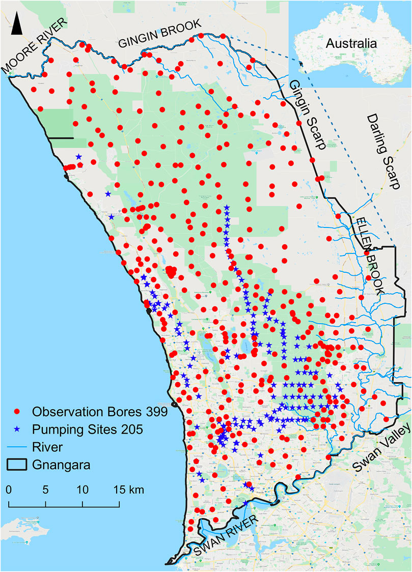
FIGURE 1. Location of the observation and pumping sites in the Gnangara region, Western Australia.

FIGURE 2

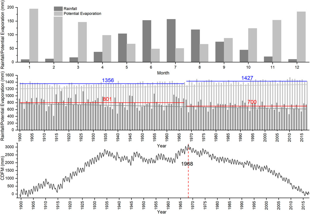
FIGURE 2. Long-term averages of the monthly rainfall, annual rainfall and potential evapotranspiration, and dry climatic periods by cumulative deviation from mean rainfall (CDFM) in the Gnangara region.

FIGURE 3

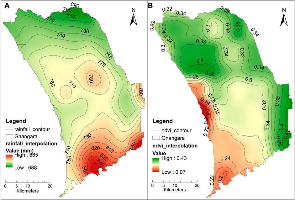
FIGURE 3. Contour map of the rainfall (A) and NDVI (B) in the Gnangara region.

In the Gnangara groundwater system, plantation forestry is one of the major land use types (land use map in 1992 and 2018 extracted from Bureau of Rural Sciences (2006) and Australian Bureau of Agricultural and Resource Economics and Sciences (2018), Supplementary Figure S1). Approximately 17,000 ha of the area contains currently mature maritime pine (Pinus pinaster) plantations, located in the centre of the system (Forest Products Commission, 2009). Mature pines consume much water because the transpiration rate of pines is 23% higher than that of the native banksia woodland surrounding the pine plantation (Carbon et al., 1982; Tremayne, 2010). Urbanized areas mainly occur in the southwest and southeast of the system. Other land use types, such as pastures, are found along the eastern and northern margins of the system (Australian Bureau of Agricultural and Resource Economics and Sciences, 2018). The long-term mean annual NDVI at various sites was adopted to determine the spatial distribution of the NDVI in the Gnangara region via the empirical Bayesian kriging in ArcGIS 10.5 (Figure 3B) (with Root Mean Squared Error of 0.003). Figure 3B shows that high NDVI values largely occurred in the north and east of the Gnangara region, which are mainly covered with pine and banksia plantations and pastures. Low NDVI were mainly found in the south and middle west of the Gnangara region where urban areas are located.

The groundwater resources in the Gnangara region are mainly from winter rain. A high proportion of the precipitation infiltrates into the soil and recharges local groundwater due to the sandy soils with a high permeability occurring in the study area (Western Australian Planning Commission, 2001). The groundwater resources are usually abstracted for public water supply purposes, private water use, park and garden watering, industrial and commercial use, horticultural and agricultural irrigation, and domestic use. Approximately 42% of the extracted groundwater is used for the public water supply (Department of Water, 2009a).

The Gnangara groundwater system comprises four different hydrogeological aquifers and the 3D Aquifer Visualization of the Gnangara region can be found in http://www.bom.gov.au/water/groundwater/explorer/3d-aquifer-visual.shtml. The shallowest, unconfined superficial aquifer (its top surface is commonly termed the Gnangara Mound) which stretches across the coastal plain, with an average thickness of 45 m, a maximum thickness of 75 m and a depth to groundwater ranging from 3 to 20 m. From east to west, the sediments of the superficial aquifer generally vary from being predominantly clayey adjacent to the Darling Fault and Gingin Scarp, to a sandy succession in the central coastal plain area, and to sand and limestone within the coastal belt. The hydraulic properties of the superficial aquifer vary significantly depending on geology. The horizontal hydraulic conductivity increased from western and eastern margin to central with values of 0.1, 15, and 50 m/day in Guildford Clay, Bassendean Sand, Tamala limestone. The shallow, semi-confined Mirrabooka aquifer which is mainly occurs in the southern and eastern regions of the Gnangara region and varies in thickness to a maximum thickness of 160 m, and its horizontal hydraulic conductivity of this aquifer ranges from 4 to 10 m/day. The deep, partially confined Leederville aquifer below the superficial aquifer, extends beneath the entire coastal plain except in the north near the Swan Estuary and in the south-east corner, and is typically several hundred meters thick, consisting of discontinuous interbedded sandstones, siltstones and shales with horizontal hydraulic conductivity of the sandstone beds about 10 m/day and that of the siltstone and shale beds about 1 × 10^–6 m/day. The Yarragadee aquifer is the deepest and major confined aquifer underlying the Perth Region and extending to the north and south within the Perth Basin. It is a multilayered aquifer often more than 2000 m thick, consisting of discontinuous interbedded sandstones, siltstones and shales with the average horizontal hydraulic conductivities range between 1 × 10^–6 and 10 m/day., and it offers a vast storage and a robust supply of groundwater (Davidson and Yu, 2008; Department of Water, 2009a; Environmental Protection Authority, 2017). The Gnangara Mound developed because the vertical rainfall infiltration rate (about 1 m/day) exceeds the horizontal groundwater flow rate (ranges from 50 m/year to 1000 m/year) in the aquifer (Davidson, 1995; Davidson and Yu, 2008). Groundwater recharge of the superficial aquifer is highly variable and depends on the local rainfall, land use, and geological conditions (Davidson and Yu, 2008; Department of Water, 2009a). The superficial aquifer is predominantly recharged by rainfall in winter with some upward recharge, occurring from the underlying Leederville and Yarragadee aquifers (Department of Water, 2009a). Groundwater is naturally discharged into wetlands, rivers, springs and ocean, and groundwater undergoes vegetation transpiration and leaks into underlying aquifers during groundwater movement. Additional discharge is associated with groundwater abstraction (Davidson and Yu, 2008; Department of Water, 2009a).

Data Source

Climate Data

Climate data (1900–2017), including the daily precipitation and FAO56 potential evapotranspiration (FAO Penman-Monteith equation, Allen et al. (1998)), were extracted from the SILO Data Drill database created by the Queensland Government Department of Science, Information Technology and Innovation (DSITI). This dataset provides 0.05° gridded daily data and are constructed by spatially interpolating the observational data with methods of a thin plate smoothing spline and ordinary kriging (Jeffrey et al., 2001) and can be accessed on the Internet at https://www.longpaddock.qld.gov.au/silo/. Minimum and maximum temperatures, solar radiation and vapor pressure prior to 1956 were interpolated by an anomaly interpolation technique (Zajaczkowski and Jeffrey, 2020). At each observation site, the acquired climate data exhibit a daily time-step and start at 20 years prior to the first observation date of the groundwater level.

Land Cover Data

The NDVI (Normalized Difference Vegetation Index) - high resolution gridded (0.05° * 0.05° grid) monthly NDVI dataset (1992–2017) used as the land cover change data in this study was obtained from the Australian Bureau of Meteorology website (http://www.bom.gov.au/metadata/catalogue/view/ANZCW0503900404.shtml). The satellite data originated from the Advanced Very High-Resolution Radiometer (AVHRR) instruments onboard the National Oceanic and Atmospheric Administration (NOAA) series of satellites operated by the US (http://noaasis.noaa.gov/NOAASIS/ml/avhrr.html). The NOAA-11, -14, -16 and -18 satellites were considered. The NDVI was used to examine the vegetation cover changes because the vegetation and non-vegetation area is easy to identify and historical land use information cannot be obtained. The NDVI value ranges from −1 to +1, where positive values indicate vegetation features and negative values indicate non-vegetation features (Gandhi et al., 2015).

Groundwater Monitoring Data

Groundwater monitoring data were retrieved from 325 observation bores in the unconfined superficial aquifer within the Gnangara region (Figure 1). The observation records are irregular and the data from 1992 to 2014 are used in this study. This dataset was provided by the Department of Water and Environmental Regulation, Government of Western Australia. The details of cite description can be downloaded for free from https://water.wa.gov.au/maps-and-data/monitoring/water-information-reporting.

Groundwater Abstraction

A groundwater abstraction dataset (2,324 pumping sites) collected from the different aquifers (mostly pertaining to from superficial aquifer) in the Gnangara region, from 1992–2014, was used in this study. These groundwater pumping data referred to the extraction for public and private water supply purposes. The groundwater abstraction data were obtained from the Department of Water and Environmental Regulation, Government of Western Australia.

Methods

The Transfer Function Noise Model

The original TFN model was developed by von Asmuth et al. (2002) to simulate the groundwater level. This model includes three components: a deterministic component simulating the groundwater level due to the combined effect of all external factors, a residual series of the groundwater level and a constant component of the local drainage level. The Pearson type III distribution function was introduced by von Asmuth et al. (2002) to establish the precipitation and evapotranspiration impulse response functions. A revised version of the Pearson type III distribution function was adopted and five weaknesses in use for climatic stressors had been improved by Peterson and Western (2014). The first modification was to minimize the parameter covariance. The second modification was the calibration reproducibility was improved by undertaking a log 10 transformation of the parameters. The third modification was to reduce the impulse response function value at the start of the climate record. The fourth modification was to address the integration of the function from the first climate observation to negative infinity. The fifth modification was minimizing rounding errors in the numerical estimation of the integrals. Finally, Eq. 1 details the linear TFN model comprising two components of precipitation and evaporation:

$h_t=\underset{-\infty }{\overset{t}{{\displaystyle \int }}}{P}_{\tau }\theta \left(t-\tau \right)d\tau -\underset{-\infty }{\overset{t}{{\displaystyle \int }}}{f}_E{E}_{\tau }\theta \left(t-\tau \right)d\tau +n_t+d(1)$

where $P_{\tau }$ [LT⁻¹] and $E_{\tau }$ [LT⁻¹] are the daily precipitation and the daily potential evapotranspiration, respectively, and $f_E$ [−] is a dimensionless parameter scaling the transfer function for application to the evapotranspiration signal. $\theta \left(t-\tau \right)$ is the impulse response function which was defined by von Asmuth and Bierkens (2005). $n_t$[L] is the residual series of groundwater level at time t, and is calculated by the observed groundwater head at time t subtracted from the modeled groundwater head at time t, d[L] is the constant component for local drainage level. To consider the groundwater level response to land cover change, von Asmuth et al. (2008) added a third integral to the time series model for the land cover change stressor, which involves a weighting the evapotranspiration integral by two parameters of the evaporation factor parameter $f_L$ that depending on the soil and land cover and the historic fraction of vegetation clearing $L_{\tau }$ (Eq. 2):

$h_t=\underset{-\infty }{\overset{t}{{\displaystyle \int }}}{P}_{\tau }\theta \left(t-\tau \right)d\tau -\underset{-\infty }{\overset{t}{{\displaystyle \int }}}{f}_E{E}_{\tau }\theta \left(t-\tau \right)d\tau -\underset{-\infty }{\overset{t}{{\displaystyle \int }}}{f}_L{L}_{\tau }{E}_{\tau }\theta \left(t-\tau \right)d\tau +n_t+d(2)$

However, the linear TFN model does not simulate the groundwater head well because of the nonlinearity between precipitation and groundwater head (Peterson and Western, 2014). Therefore, a vertically lumped soil moisture model (Eq. 3) was introduced into Eq. 1. The model is highly flexible and contains one to five parameters (KlemeŠ, 1986).

$\frac{dS}{dt}=\text{P}{\left(1-\frac{S}{\widehat{S_{cap}}}\right)}^{\alpha }-\widehat{k_{sat}}{\left(\frac{S}{\widehat{S_{cap}}}\right)}^{\widehat{\beta }}-E_t{\left(\frac{S}{\widehat{S_{cap}}}\right)}^{\gamma }(3)$

where S [L] is the soil moisture at time $t$ [T], $\widehat{S_{cap}}$ [L] is the antilog (log10)-transformed parameter related to the maximum soil moisture capacity $S_{cap}$ [L], $\widehat{k_{sat}}$ [LT⁻¹] is the antilog (log10)-transformed parameter related to the maximum vertical soil saturated conductivity $k_{sat}$ [LT⁻¹], $E_t$ [LT⁻¹] is the potential evapotranspiration rate at time $t$, $\alpha$ is a dimensionless parameter controlling the fraction of precipitation available for infiltration as the catchment wetness, $\widehat{\beta }$ is the antilog (log10) transformed dimensionless parameter controlling the free drainage as the catchment wetness, and $\gamma$ is a dimensionless parameter controlling soil evapotranspiration.

In the process of transforming the precipitation and potential evapotranspiration time series data into the required TFN model input, the precipitation $P_{\tau }$ in Eq. 1 can be replaced with the free drainage ${\left(\frac{S}{\widehat{S_{cap}}}\right)}^{\widehat{\beta }}$ or infiltration rate ${\left(1-\frac{S}{\widehat{S_{cap}}}\right)}^{\alpha }$, and the potential evapotranspiration $E_t$ can be replaced with the soil evapotranspiration ${\left(\frac{S}{\widehat{S_{cap}}}\right)}^{\gamma }$or groundwater potential evapotranspiration$E_t\left(1-\frac{S}{\widehat{S_{cap}}}\right)$. Two impulse response functions ${\theta }_P$ and ${\theta }_E$ for precipitation and evapotranspiration, respectively, were adopted in the time series model.

To consider for the groundwater level response to groundwater pumping, Shapoori et al. (2015a) and Shapoori et al. (2015c) added a third integral to the time series model (Eq. 4). Shapoori et al. (2015c) showed that models with and without groundwater evaporation produced similar results. Therefore, the second integral of groundwater evaporation was omitted in the models of this study.

$h_t=\underset{-\infty }{\overset{t}{{\displaystyle \int }}}{\left(\frac{S}{\widehat{S_{cap}}}\right)}^{\widehat{\beta }}{\theta }_P\left(t-\tau \right)d\tau -\underset{-\infty }{\overset{t}{{\displaystyle \int }}}{E}_t\left(1-\frac{S}{\widehat{S_{cap}}}\right){\theta }_E\left(t-\tau \right)d\tau -\underset{-\infty }{\overset{t}{{\displaystyle \int }}}{Q}_{\tau }{\theta }_{H\parallel F}\left(t-\tau \right)d\tau +n_t+d(4)$

where $Q_{\tau }$ [L³T⁻¹] is the daily pumping rate. The response function ${\theta }_{H\parallel F}$ can either be the Hantush’s equation for a leaky aquifer (Hantush, 1956; Eq. 5) or the Ferris and Knowles’ well equation for a nonleaky aquifer (Ferris and Knowles, 1963; Eq. 6). The Ferris and Knowles’ well equation without groundwater potential evapotranspiration was selected in this study due to the groundwater levels in most bores occurring deeper than 1 m according to tests conducted by Shapoori et al. (2015a):

${\theta }_H\left(t\right)=\frac{a}{t}exp\left(-\frac{b^2}{t}-c^{2}t\right)(5)$

${\theta }_F\left(t\right)=\frac{a}{t}exp\left(-\frac{b^2}{t}\right)(6)$

where a, b and c are parameters that only have a physical meaning if the basic Hantush assumptions are satisfied.

According to Peterson and Western (2014), there are 84 nonlinear TFN models based on 16 soil moisture models available within HydroSight. Eqs 3, 7 (Peterson and Western, 2014), Eq. 8 (Peterson and Western, 2014), and Eq. 9 (Siriwardena et al., 2011) are four model structures used in this study and is named as structure “cccc,” “c1c1,” “c0cc,” “inf101.” Structure cccc means all parameters are calibrated. Structure c1c1 means fixing $\alpha$ = $\gamma =1$. Structure c0cc means fixing $\alpha$ = $1$. Structure inf1c1 means fixing $\alpha$ = $\gamma =1 and \beta =0$. Free drainage was chosen to transform the precipitation time series data into the required TFN model input. The Ferris and Knowles’ well equation was selected as the response function.

$\frac{dS}{dt}=\text{P}\left(1-\frac{S}{\widehat{S_{cap}}}\right)-\widehat{k_{sat}}{\left(\frac{S}{\widehat{S_{cap}}}\right)}^{\widehat{\beta }}-E_t\left(\frac{S}{\widehat{S_{cap}}}\right)(7)$

$\frac{dS}{dt}=\text{P}-\widehat{k_{sat}}{\left(\frac{S}{\widehat{S_{cap}}}\right)}^{\widehat{\beta }}-E_t\left(\frac{S}{\widehat{S_{cap}}}\right)(8)$

$\frac{dS}{dt}=\text{P}\left(1-\frac{S}{\widehat{S_{cap}}}\right)-E_t\left(\frac{S}{\widehat{S_{cap}}}\right)(9)$

Model Calibration and Evaluation

Following Shapoori et al. (2015a) and Shapoori et al. (2015c), the first 70% and last 30% of the observation records were designated as the calibration and evaluation periods, respectively. To identify individual parameter which produces the best possible fit to the hydrograph, the default calibration methods in the toolbox of Shuffled Complex Evolution with Principal Components Analysis - the University of California at Irvine (SP-UCI), developed by Chu et al. (2011), were used. SP-UCI is a global optimization algorithm based on the Shuffled Complex Evolution (SCE-UA) method (Duan et al., 1992) to address high-dimensional and complex problems.

Model Performance Assessment

The Akaike information criterion with correction (AICc) and Bayesian information criterion (BIC) (Burnham and Anderson, 2004) were used to account for the number of model parameters. The lower AICc and BIC indicates the better model. Moreover, the Nash-Sutcliffe efficiency (NSE) has been widely used to assess the goodness fit of a hydrograph (Ritter and Muñoz-Carpena, 2013; van der Spek and Bakker, 2017). Therefore, to assess the TFN model performance, the NSE (Nash and Sutcliffe, 1970) and unbiased NSE (Shapoori et al., 2015a) were adopted in the calibration and evaluation periods, respectively. NSE ranges from −∞ to 1. The model is more accurate when the NSE value is closer to 1. At NSE = 1, the modelled data are a perfect match to the observed data (only if the measurements are free of errors). At NSE = 0, the modelled data are as accurate as the mean of the observed, and if NSE <0, the modelled data are less accurate than the mean observed data. Model performance can be evaluated as unsatisfactory if NSE ≤ 0.5, model performance can be evaluated as satisfactory if 0.50 < NSE≤0.65; model performance can be evaluated as good if 0.65 < NSE≤0.75; model performance can be evaluated as very good if 0.75 < NSE≤0.1 (Moriasi et al., 2007; Moriasi et al., 2015).

Radius of Influence

Based on the current data on the study area, the Dupuit equation (Dupuit, 1863) was selected to calculate the radius of influence of pumping wells. In the confined aquifer, the Dupuit equation (Eq. 10) was used to calculate the radius of influence of pumping wells. In the unconfined aquifer, the Dupit equation (Eq. 11) (Dupuit, 1863) was used to calculate the radius of influence of pumping wells.

$\text{r}={10}^{\frac{s_1{\log }_{10}{r}_2-s_2{\log }_{10}{r}_1}{\left(s_1-s_2\right)}}(10)$

$\text{r}={10}^{\frac{s_1\left(2H-s_1\right){\log }_{10}{r}_2-s_2\left(2H-s_2\right){\log }_{10}{r}_1}{\left(s_1-s_2\right)\left(2H-s_1-s_2\right)}}(11)$

where $\text{r}$ [m] is the radius of influence of a pumping bore, $s_1$ and $s_2$ [m] are the drawdowns in the observation bores, $r_1$ and $r_2$ [m] are the distances between the observation and pumping bores, and $H$ [m] is the thickness of the aquifer. In this study, the thickness of the unconfined aquifer was determined according to Smith and Pollock (2010).

Results

Model Structure Comparison

To determine the most applicable model structure, four soil moisture model structures (structures cccc, c1c1, cocc and inf101) were tested in all bores for climate-only analysis. For AICc and BIC, there are not obvious differences between these four model structures, but structure cccc showed worse than other three model structures (Figure 4A). The climate-only analysis means the groundwater level is considered only influenced by rainfall. The NSE values of 325 bores using these four soil moisture models are listed in a box plot is shown in Figure 4B. During the calibration period, model structure inf101 performed the worst, with the lowest mean, median values of the NSE. The model structure cccc performed the best with the highest mean value of NSE in calibration but performed the worst with the lowest mean value of NSE. The model structure c0cc performed as good as model structure c1c1. Therefore, either model structure c1c1 with less parameters than c0cc was appropriate in this study. In this study, model structure c1c1 (Eq. 7) was chosen to model all the bores in the Gnangara region in all subsequent groundwater level analyses.

FIGURE 4

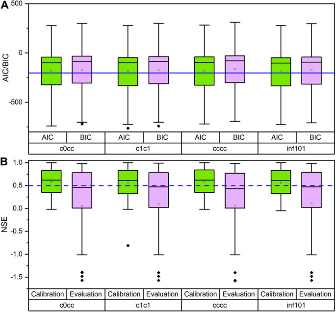
FIGURE 4. Box plot of AICc, BIC (A) and NSE (B) results of the four soil model structures in the climate-only analysis. Note: Structure cccc means all parameters of $k_{sat}$, α, β, and γ are calibrated. Structure c1c1 means α = γ = 1. Structure c0cc means α = 1. Structure inf101 means α = γ = 1 and β = 0.

Model Performance

Climate Only

Sixty percent of the bores in climate-only (C) analysis during the calibration period produced an acceptable performance (NSE >0.5), of which 36% of the bores performed very good, 10% of the bores performed good and 14% of the bores performed satisfactorily. In addition, 40% of the bores performed unsatisfactorily. During the evaluation period, 48 and 52% of total bores yielded an acceptable and unsatisfactory groundwater head modelling performance, respectively.

Spatially, bores producing an acceptable model performance in climate-only analysis predominantly occurred in the southeastern Gnangara, followed by the northern Gnangara, and an unsatisfactory performance was predominantly produced in central-western and northwestern Gnangara and the coastal area of the Gnangara region during the calibration period (Supplementary Figure S2). The spatial distribution of model performance during the evaluation period is similar with that during the calibration period. However, an unsatisfactory performance increased in south area of the Gnangara region (Supplementary Figure S2).

Climate and Land Cover

The model performance was improved during both the calibration and evaluation periods when the NDVI was added to the TFN model. The acceptable performance increased from 60 to 62%, especially the good and satisfactory performance level with an improvement of 2% during the calibration period. In addition, the unsatisfactory performance level was reduced by 2% during the calibration period. However, the acceptable performance level decreased from 48 to 47% during the evaluation period.

Among the 325 bores in the Gnangara region, an acceptable performance was largely attained in the south, southeast and north of the Gnangara region during the calibration and evaluation periods in the climate and land cover (C + L) analysis (Supplementary Figure S2). An unsatisfactory performance during the calibration and evaluation periods was predominantly distributed is mainly attained in the central-western and northwest of the Gnangara region (Supplementary Figure S2).

Figure 5 shows the spatial distribution and magnitude of the NSE improvement considering the land cover data were considered. The improvement was calculated by subtracting the NSE value of the climate-only analysis from the NSE value of the climate and land cover analysis. The model performance had decreased when the NSE change value was smaller than −0.1. The model performance remained stable when the NSE change value varied between −0.1 and 0.1. The model performance had improved when the NSE change value was larger than 0.1. During the calibration period, the NSE value at 17 bores had improved with the NSE change values ranging from 0.1 to 1.85 and 18 bores had been reduced by values ranging from −8.62 to −0.1. Most of the bores (290) remained stable, with NSE change values ranging from -0.1 to 0.1. During the evaluation period, the NSE value at 21 bores had improved with NSE change values ranging from 0.1 to 0.85, and at 19 bores, the performance had decreased with NSE change values ranging from -0.52 to −0.1. Most of the bores (285) remained stable, with NSE change values ranging from −0.1 to 0.1. In calibration and evaluation period, the NSE improved mainly at bores in northern Gnangara and the NSE declined mainly at bores in the northern parts of the Gnangara region.

FIGURE 5

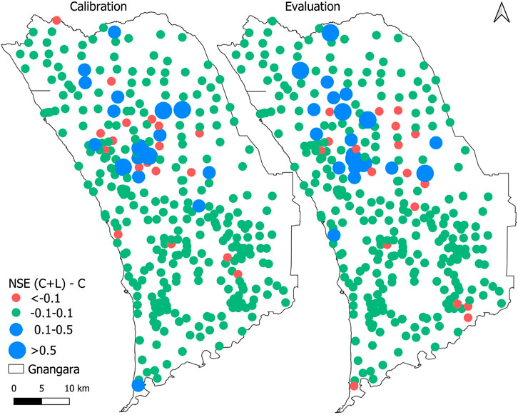
FIGURE 5. Difference in NSE between the climate-only (C) analysis and the climate and land cover (C + L) analysis.

Climate and Groundwater Pumping

According to the empirical Dupuit equation, the radius of influence of the pumping wells in the confined and unconfined aquifers ranged from 708 to 9,303 m, and 1,302 pumping sites were determined to influence 271 observation sites. At these 271 observation sites, the groundwater pumping stressor was included to assess its contribution to the groundwater level changes. The corresponding modelling results of the C analysis and C + L analyses were separated and compared to climate and pumping analysis (C + P) results during the calibration and evaluation periods.

To validate the pumping well influence on the groundwater head, models with multiple bores and only the nearest bore were applied. The NSE of these two models are shown in Figure 6. During both the calibration and evaluation periods, the models containing one bore and multiple bores did not exhibit notable differences, but the model with one bore attained a slightly better performance than the model with multiple bores. Therefore, the model with one bore was applied in the climate and pumping stressor analysis.

FIGURE 6

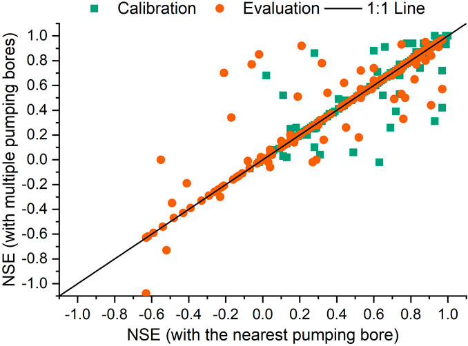
FIGURE 6. Comparison NSE results between the climate and pumping analysis with the nearest pumping bore and multiple pumping bores.

During the calibration period, 60% of the bores produced an acceptable modelling performance, and 40% of the bores produced an unsatisfactory modelling performance in the C analysis (Figure 7). The acceptable model performance level had been improved by 3 and 19% in the C + L and C + P analyses, respectively. Especially for the very good performance rate had improved by 21% in the C + P analyses (Figure 7). Moreover, unsatisfactory model performance rate has been reduced by 2 and 18% for C + L and C + P analysis. During the evaluation period, the acceptable model performance rate increased slightly from 48% in the C analysis to 50% in the C + P analysis. In the C + L analyses, the acceptable model performance rate was even reduced by 3% (Figure 7). In general, the pumping analysis results were slightly better than the land cover analysis results during both the calibration and evaluation periods.

FIGURE 7

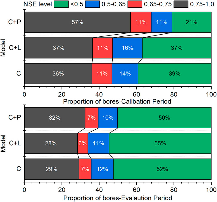
FIGURE 7. Proportion of bores with different NSE levels of the climate-only (C) analysis, climate and land cover (C + L) analysis, and climate and pumping (C + P) analyses.

Among the 271 bores in the Gnangara region, an acceptable and unsatisfactory model performance predominantly occurred in the south and north (coastal region), respectively, of the study area in the C analysis (Supplementary Figure S3). In central and north area, the model performance level increased when the pumping stressor were considered (Supplementary Figure S3). The model performance level was improved at a few bores in north area for C + L analysis. During the evaluation period, the unsatisfactory performance level was much higher that during the calibration period, especially in the bores of central, coastal and north part (Supplementary Figure S3).

Figure 8 shows the spatial distribution and magnitude of the NSE improvement when the land cover and pumping data were considered. The improvement was calculated by subtracting the NSE value of the climate-only analysis from the NSE value obtained when the land cover and pumping data were included in the model, respectively. During the calibration period, most of the bores (140) remained stable, with NSE values ranging from −0.1 to 0.1. At 18 bores, the performance improved with NSE change values ranging from 0.1 to 0.85, and at 17 bores, the performance decreased with NSE change values ranging from −0.52 to −0.1 in the C + L analyses. During the evaluation period, 15 bores with an increased NSE value were found, with the NSE improvement ranging from 0.1 to 1.85, while 16 bores with a reduced NSE value were found with NSE reduction ranging from −0.1 to -8.62 during the calibration period. And 240 bores keep a stable NSE values. In the C + P analysis, the number of bores with an increased NSE in both the calibration (98, range: 0.1–0.98) and evaluation periods (59, range: 0.1–27.27) was larger than that in the C + L analysis. Moreover, the number of bores with an NSE reduction increased to 59 during the evaluation periods (range: 9.82∼−0.1) compared to that during the calibration (15 bores) period. The bores with an NSE improvement in the C + L analysis were largely distributed in the upper part of the bores area during the calibration and evaluation periods (Figure 8). The bores with an NSE reduction and increase in the C + L analysis were mainly foundin north area of the Gnangara region. In the C + P analysis, the areas in the southwestern Gnangara with a high concentration of pumping wells, the model performance level did not exhibit a notable improvement. Areas with an NSE improvement primarily occurred in the north and central area of the Gnangara region.

FIGURE 8

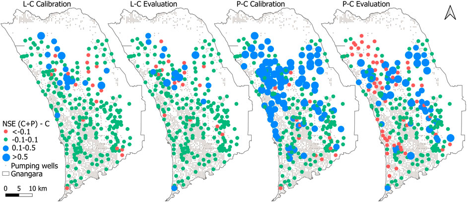
FIGURE 8. Improvement in NSE of the climate and land cover, and the climate and pumping analyses.

Drivers’ Contribution

Contribution in Space

To determine the spatial distribution of the contribution of each stressor to the groundwater level changes, the multiyear average rainfall, land cover, and pumping contribution rate of bores with NSE exceeding 0.5 (acceptable model performance) during both the calibration and evaluation periods were used to generate the spatial distribution of the contribution rate in the Gnangara region by the Inverse Distance Weighted method in ArcGIS 10.1 (Figures 9, 10).

FIGURE 9

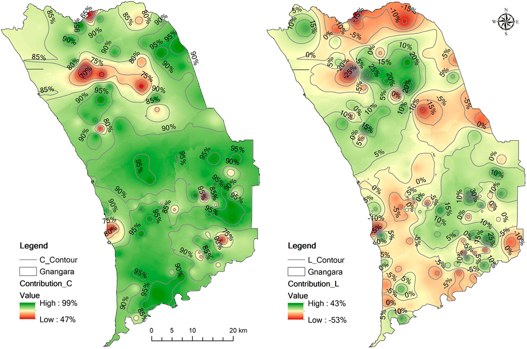
FIGURE 9. Spatial distribution of the rainfall and land cover (as suggested by the NDVI) contributions to the groundwater level changes in the Gnangara region.

FIGURE 10

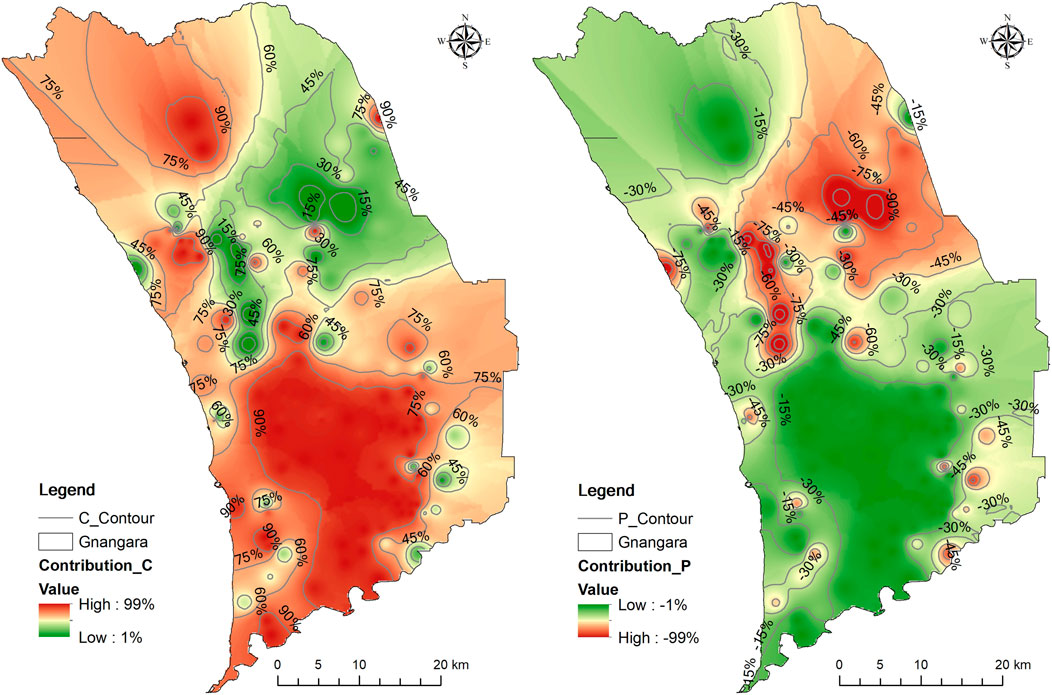
FIGURE 10. Spatial distribution of the rainfall and pumping contributions to the groundwater level changes in the Gnangara region.

As shown in Figure 9, the multi-year mean contributions of rainfall and land cover to the groundwater level changes ranged from 44 to 99% and from -53 to 43%, respectively. A large rainfall contribution rate was mainly found in central and southern Gnangara region. In contrast to the rainfall recharge contribution, the land cover contribution can either be positive or negative. A positive land cover contribution (green area) was largely distributed in upper central and southeastern Gnangara region. In certain areas, such as the southwestern and central-western areas (light yellow area), the land cover contribution was very small. In the south-western, north margin, central-eastern parts (red areas) of Gnangara region, the contribution was negative.

As shown in Figure 10, the multi-year mean contributions of rainfall and pumping to the groundwater level changes ranged from 1 to 99% and from −1% to −99%, respectively. Large rainfall recharge contribution to the groundwater level changes mainly occurred in the southwestern and northwestern parts of the Gnangara region. In contrast to the rainfall recharge contribution, the pumping contribution to the groundwater level changes was negative. The bores most affected by pumping occurred in the north-eastern parts of the Gnangara region.

Contribution in Time

Over time, the multi-site mean contributions of climate change and land cover on groundwater level were 90 and 2% with ranges of 89–90% and 2.1–2.3%, respectively. The multi-site mean contributions of climate change and pumping were 77% and -23% with ranges of 68–99% and −1%∼−32%, respectively. In the whole Gnangara region, the trend of the rainfall contribution slightly decreased from 1992 to 2014 (Figure 11A). The land cover contribution rate was stable from 1992 to 2014. The pumping contribution rate decreased from 1992 to 2014. However, the pumping contribution rate is negative, that means the pumping activities lowers the groundwater decline. Moreover, the trend of the contribution of factors on groundwater level were calculated. Seventy-four percent of the rainfall contribution rate trend showed decline (<=−0.01) over time and 26% of the rainfall contribution rate trend showed stable (0) for C + L analysis. Eighteen percent of the land cover contribution rate trend showed decline over time, 70% of the land cover contribution rate trend showed stable, and 12% of the land cover contribution rate trend showed increase (≥0.01) for C + L analysis. Sixty percent of the rainfall contribution rate trend showed decline over time and 40% of the rainfall contribution rate trend showed stable for C + P analysis. Fifty-eight percent of the pumping contribution rate trend showed decline over time, 42% of the pumping contribution rate trend showed stable for C + P analysis.

FIGURE 11

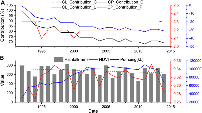
FIGURE 11. Contribution rates in the climate-only (C), climate and land cover (C + L), and climate and pumping (C + P) analyses to the groundwater level changes (A). Rainfall, NDVI and groundwater pumping in the Gnangara region (B).

Model Parameters

The variability of critical fitted parameters of the model was presented in a box plot (Figure 12) and the spatial distribution of the fitting parameters was presented in Figure 13. Figure 12 showed that the Ksat, β, and Scap between C + L and C + P analysis is slight. Parameter of Ksat (maximum vertical conductivity) ranged from 0.01 to 10 m/day with mean of 0.47 and 0.61 m/day for C + L and C + P analysis, respectively. Parameter of β(power term for drainage rate) ranged from 1 to 10 with mean of 3.59 and 3.56 for C + L and C + P analysis, respectively. Parameter of Scap (soil moisture storage capacity) ranged from 0.01 to 1 m with mean of 0.18 and 0.21 m for C + L and C + P analysis, respectively. Spatially, Figure 13 showed about 60% bores has the Ksat of 0.01–0.2 m/day for both C + L and C + P analysis. And larger Ksat (more than 2 m/day) was found in the northern Gnangara for C + L analysis and in both southern and northern Gnangara for C + P analysis. Parameter of β in spatial showed slight difference between C + L and C + P analysis and the larger β is mainly occurred in the north area of the Gnangara region. 84 and 76% bores has the Scap of 0.01–0.2 m. The bores with Scap larger than 0.4 m is dispersedly distributed in the study area.

FIGURE 12

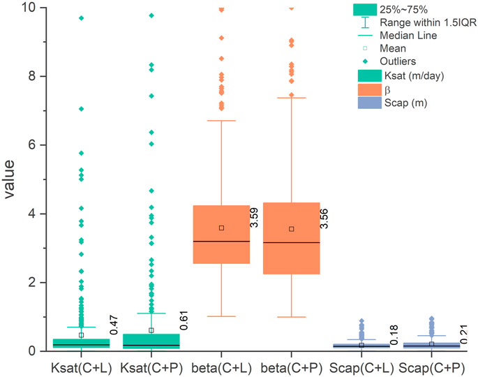
FIGURE 12. Box plot of the calibrated parameters of the model.

FIGURE 13

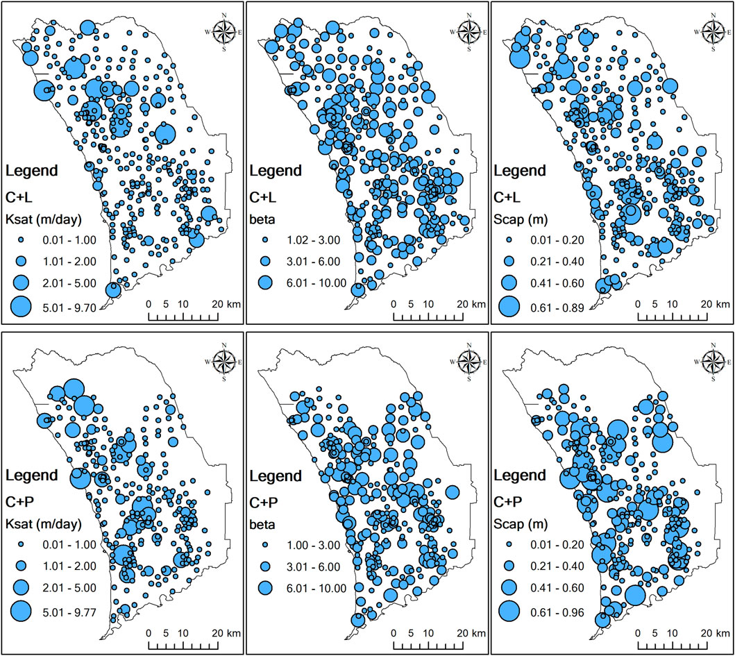
FIGURE 13. Spatial distribution of the calibrated parameters of the model.

Discussion

Groundwater Hydrograph Decomposition Evaluation

The spatial distribution of the acceptable model performance level (in the southern Gnangara) in the climate-only analysis was consistent with the area with a high rainfall. Additionally, the areas with a large rainfall recharge contribution were largely found in the area with a high rainfall (Figure 3), while a small rainfall recharge contribution occurred in the area with a low rainfall. The rainfall always keeps higher contribution (47–99 and 1%–99%) than land cover (−53–43%) and groundwater pumping (−1% to −99%) contribution after the NDVI and groundwater pumping were included into the model, respectively. Generally, the area rainfall more than 770 mm have the contribution rate more than 75%. These results indicated that the spatial distribution of the rainfall recharge contribution to groundwater was consistent with the rainfall distribution based on a comparison of the rainfall recharge contribution graph (Figures 9, 10) and rainfall graph were compared (Figure 3). Temporally, the rainfall contribution rate continually decreased and were higher than land cover and pumping contribution rate (Figure 11A), which is closely related to the rainfall reduction over time (Figure 11B). All of the above results indicate that the climate (precipitation) is the main factor influencing the groundwater level in the Gnangara region (dominating the groundwater level changes). Yesertener (2005) and Gallardo (2013) also proposed that climate change is the primary factor influencing the groundwater level decline in the Gnangara region based on the cumulative deviation from main rainfall (CDFM) analysis method. This finding has been verified, and the contribution of climate change to the groundwater level changes in time and space have been quantified.

The model performance was improved at some bores in northern Gnangara when the land cover data were added to the model, indicating that the land cover change also exerts an impact on groundwater level changes. However, the land cover contribution on groundwater level was stable over time and the contribution rate kept at 2%. Although the land cover had changed in some area over time, the NDVI changes for the whole region is little (Figure 11B). This demonstrated that the land cover changes had influence on local long-term groundwater level changes, but the influence is limited and is stable over time. The locations of the sites with an improved model performance generally agreed with the vegetated area in the northern Gnangara region (suggested by high NDVI) (Figure 3B). In the central of the northern Gnangara region, the land cover contribution rate was higher and the NDVI was lower than surrounding areas, indicating a negative relationship between land cover changes and groundwater level changes. These indicated that the groundwater level in the northern Gnangara region was closely related to the local vegetation conditions. Although the land cover contribution rate is positive in central of the northern Gnangara region, the positive trend over time was decreasing because of the increased areas of conservation and natural environments, especially the minimal use area (Bureau of Rural Sciences, 2006; Australian Bureau of Agricultural and Resource Economics and Sciences, 2018). In the margin of northern Gnangara region, the land cover changes lower the groundwater level due to the land use of grazing modified pastures reduced and the other minimal land use increased (Bureau of Rural Sciences, 2006; Australian Bureau of Agricultural and Resource Economics and Sciences, 2018). The plantation forests area reduced from 1992 to 2018 (Bureau of Rural Sciences, 2006; Australian Bureau of Agricultural and Resource Economics and Sciences, 2018). However, in the plantation forests area in land use map 2018, the land cover contribution rate is up to −53%. This is likely closely associated with the high density of pine plantations in these areas (Yesertener, 2007; Gallardo, 2013). In the southwestern area of the Gnangara region, urban use is the main land use, but the contribution is negative, that means other factors such as groundwater abstraction influenced the groundwater level.

The model performance was significantly improved after the pumping data were added to the model. In the south area of the study area, the model performance remained high. In the western part of the study area, which is the coastal region, the model performance remained unsatisfactory, although the land cover or pumping data were included. In the coastal areas, the climate, land cover and pumping exert limited impacts on the groundwater level changes, and other factors such as seawater intrusion, may impose major impact on the groundwater level changes. The limited changes in the groundwater level along the coast also occur due to the extremely high hydraulic conductivity of the Tamala limestone and proximity to the discharge zone (Costall et al., 2020). Other possibility of limited groundwater level changes may be from the boundary conditions (Morgan et al., 2012). As the C, C + L, and C + P analysis results indicated, the model performance was improved when the pumping data were considered, especially during the calibration period. However, the model performance was slightly improved when the land cover data were considered, and the performance at some sites was reduced. Moreover, the large pumping contribution (negative) to the groundwater level changes occurred in the northeast of the Gnangara region and did not always occur near the pumping sites, indicating that the distance between the bores and pumping wells and the density of the pumping wells are not critical elements in the determination of the pumping contribution to the groundwater level changes. In the southwestern Gnangara, the contribution rate mainly ranged between −15% and −40% (Figure 10). However, the groundwater pumping contribution continually increased over time due to the sustained groundwater abstraction (Figure 11B). It is obvious that groundwater pumping is highest in the 2011, and the pumping contribution on groundwater level is also highest with contribution value of −32% (Figure 11B). Results indicated that sustained groundwater pumping over time has a significant influence on groundwater level decline. Depletion of groundwater levels is a global phenomenon and is defined as long term water level declination caused by sustained groundwater pumping over time (Tularam and Krishna, 2009). More attention should be paid to manage the groundwater pumping activities to ensure the sustainable use of groundwater.

The fitted parameter of the maximum vertical conductivity of the model in this study has a value range 0.01–9.8 m/day and the maximum vertical conductivity of most of the bores is concentrated in range of 0.01–2 m/day. Salama et al. (2005) and Department of Water (2009b) calculated the hydraulic conductivity in the Gnangara, ranging from 0.56 to 6.38 m/day and from 0.01 to 5 m/day, respectively. The similar results indicated the results of fitted parameters of the maximum vertical conductivity is accepted and the results of the model are credible. Moreover, the fitted parameter of Ksat and Scap showed slight difference in C + L and C + P analysis, indicating that the maximum vertical conductivity and soil moisture storge capacity are important parameter of the model.

Uncertainties and Limitations

The approach adopted in this study is based on various assumptions and has limitations, which constrain the results of the groundwater hydrograph decomposition. It should be noted that this method assumes that the drivers (climate, land cover, and groundwater pumping) of the groundwater level changes are independent of each other, and the land cover and pumping were added into the model, respectively. However, the considered drivers interact with each other, which may complicate the evaluation results. Climate change (rainfall change) could lead to changes in vegetation, thus affecting groundwater recharge, and groundwater pumping may lead to groundwater level changes, thereby negatively impacting vegetation (Şen, 2015). Many factors influence groundwater level changes, but only three major drivers were considered to establish the model in this study. Other drivers such as bush fires, pine clearing, and groundwater evaporation, were not examined. And the surface water-groundwater interaction is also an important cause of groundwater level changes in many areas (Wang et al., 2014). Moreover, this model assumed that the aquifer is homogeneous, but the thickness, permeability and water-bearing structure of the aquifer affect the accuracy of the modelling results.

In this study, model was constructed for each individual observation bore of the Gnangara region. Then, for the whole Gnangara region, the groundwater level changes and its main factors can be assessed by interpolating the results of each bore. In the model construction, an optimal model structure fitted for the study area was used for each model to reduce the model running time and improve the model operation efficiency. In fact, one model structure cannot ensure the satisfactory model results of each site. Therefore, model performance in spatial is not always satisfactory. However, in the process of interpolation, only the satisfactory model performance was used to reduce the errors in spatial.

Other limitations arise from the dataset used. NDVI was selected as the representation of the land cover impact on the groundwater level changes. The NDVI may not be accurate enough to express all of the land cover situation. However, the vegetation and non-vegetation area is easy to identify and historical land use information cannot be obtained. Furthermore, the groundwater level data at certain sites were fragmented or the number of observations was insufficient, but the established models allowed the simulation of irregular water level observations.

Conclusion

Understanding and interpreting changes in groundwater level is essential for long term management of both a groundwater resource and urban development. The present study quantitatively clarifies the impacts of three drivers, namely, climate change, land cover change and groundwater pumping (for public and private use) on the long-term groundwater level changes with HydroSight model. And the unconfined aquifer of Gnangara region in Western Australia was used as a case study.

Based on the three established independent models (climate-only analysis, climate and land cover analysis, and climate and pumping analysis models), climate always plays the most important role and positively contributes to the observed groundwater level changes. And groundwater decline in this region is mainly caused by the reduction in rainfall recharge over time. In the whole region, the contribution of the groundwater pumping to groundwater level decline is larger than that of land cover change. Temporally, from 1992 to 2014, the contribution of rainfall on the groundwater level of the Gnangara region decreased because the rainfall decreased over time. The mean pumping contribution rate is −23%, and the impact of groundwater pumping on the groundwater level decline continually increased from 1992 to 2014 because of the sustained groundwater pumping. The land cover changes had influence on long-term groundwater level changes, but the influence is limited and is stable over time with contribution rate of 2%. Spatially, in the southern Gnangara region, the groundwater level changes were mainly influenced by rainfall and pumping activities. In the northern Gnangara region, the groundwater level changes were influenced by the combination of rainfall, land cover and groundwater pumping.

The results of this study suggest that the improved groundwater hydrograph decomposition method is effective and can be easily applied in other regions due to its highly flexible. And this method improved the efficiency of data utilization, especially for the region which the groundwater head record is irregular. And the best-fit model for a certain study area can be obtained by trying different model structures. The findings of this study have important implications for research on the influence of various drivers on groundwater level changes and also provide notable guidance for local governments to rationally allocate and utilize groundwater resources. In areas where the groundwater level is mostly affected by groundwater pumping, other water resources should be utilized, such as rainfall runoff collected during the wet season for park irrigation, seawater desalinized, and surface water quality improved, while the groundwater abstraction reduction could ease the stress resulting from groundwater level decline.

Data Availability Statement

The original contributions presented in the study are included in the article/Supplementary Material, further inquiries can be directed to the corresponding author.

Author Contributions

FK contributed to the conceptualization, ideas, methodology, software programming, validation, original paper draft and visualization. JS supervised the project, helped results analysis, contributed to financial support. RSC, OB, DS and JPP contributed to study area definition, methods selection and results discussion. All authors contributed to manuscript revision, read, and approved the submitted version.

Funding

This study was jointly supported by the Key Research and Development Program of Shaanxi (Grant No. 2019ZDLSF05-02).

Conflict of Interest

The authors declare that the research was conducted in the absence of any commercial or financial relationships that could be construed as a potential conflict of interest.

Publisher’s Note

All claims expressed in this article are solely those of the authors and do not necessarily represent those of their affiliated organizations, or those of the publisher, the editors and the reviewers. Any product that may be evaluated in this article, or claim that may be made by its manufacturer, is not guaranteed or endorsed by the publisher.

Acknowledgments

The first author acknowledges the Chinese Scholarship Council for supporting his Ph.D. study at CSIRO Land and Water.

Supplementary Material

The Supplementary Material for this article can be found online at: https://www.frontiersin.org/articles/10.3389/fenvs.2021.736400/full#supplementary-material

References

Abiye, T., Masindi, K., Mengistu, H., and Demlie, M. (2018). Understanding the Groundwater-Level Fluctuations for Better Management of Groundwater Resource: A Case in the Johannesburg Region. Groundwater Sustainable 7, 1–7. doi:10.1016/j.gsd.2018.02.004

CrossRef Full Text | Google Scholar

Allen, R. G., Pereira, L. S., Raes, D., and Smith, M. (1998). Crop Evapotranspiration-Guidelines for Computing Crop Water Requirements-FAO Irrigation and Drainage Paper 56. Fao. Rome 300 (9), D05109.

Google Scholar

Australian Bureau of Agricultural and Resource Economics and Sciences (2018). Catchment Scale Land Use Mapping for Western Australia 2018, Canberra, Australia: Department of Agriculture and Water Resources: Australian Bureau of Agricultural and Resource Economics and Sciences. [Dataset].

Bekesi, G., McGuire, M., and Moiler, D. (2009). Groundwater Allocation Using a Groundwater Level Response Management Method-Gnangara Groundwater System, Western Australia. Water Resour. Manage. 23 (9), 1665–1683. doi:10.1007/s11269-008-9346-5

CrossRef Full Text | Google Scholar

Bureau of Rural Sciences (2006). 1992/93 Land Use of Australia, Version 3, Canberra: Bureau of Rural Sciences. [Dataset]

Burnham, K. P., and Anderson, D. R. (2004). Multimodel Inference. Sociol. Methods Res. 33 (2), 261–304. doi:10.1177/0049124104268644

CrossRef Full Text | Google Scholar

Carbon, B. A., Roberts, F. J., Farrington, P., and Beresford, J. D. (1982). Deep Drainage and Water Use of Forests and Pastures Grown on Deep Sands in a Mediterranean Environment. J. Hydrol. 55 (1), 53–63. doi:10.1016/0022-1694(82)90120-2

CrossRef Full Text | Google Scholar

Cheng, L., Zhang, L., Chiew, F. H. S., Canadell, J. G., Zhao, F., Wang, Y.-P., et al. (2017). Quantifying the Impacts of Vegetation Changes on Catchment Storage-Discharge Dynamics Using Paired-Catchment Data. Water Resour. Res. 53 (7), 5963–5979. doi:10.1002/2017WR020600

CrossRef Full Text | Google Scholar

Chu, W., Gao, X., and Sorooshian, S. (2011). A New Evolutionary Search Strategy for Global Optimization of High-Dimensional Problems. Inf. Sci. 181 (22), 4909–4927. doi:10.1016/j.ins.2011.06.024

CrossRef Full Text | Google Scholar

Costall, A. R., Harris, B. D., Teo, B., Schaa, R., Wagner, F. M., and Pigois, J. P. (2020). Groundwater Throughflow and Seawater Intrusion in High Quality Coastal Aquifers. Sci. Rep. 10 (1), 9866. doi:10.1038/s41598-020-66516-6

PubMed Abstract | CrossRef Full Text | Google Scholar

Davidson, W. A., and Yu, X. (2008). “Perth Regional Aquifer Modelling System (PRAMS) Model Development: Hydrogeology and Groundwater Modelling,” in Hydrogeological Record Series HG 20 (Western Australia: Department of Water, Government of Western Australia).

Google Scholar

Davidson, W. A. (1995). Hydrogeology and Groundwater Resources of the Perth Region, Western Australia. Perth, Western Australia: Geological Survey of WA.

Department of Water (2009a). “Gnangara Groundwater Areas Allocation Plan,” in Water Resource Allocation Planning Series (Perth, Western Austrlia: Department of Water, Government of Western Australia).

Google Scholar

Department of Water (2009b). “Perth Regional Aquifer Modelling System (PRAMS) Model Development_ Calibration of the Coupled Perth Regional Aquifer Model PRAMS 3.0,” in Hydrogeological Record Series HG 28 (Western Australia: Department of Water).

Google Scholar

Döll, P. (2009). Vulnerability to the Impact of Climate Change on Renewable Groundwater Resources: a Global-Scale Assessment. Environ. Res. Lett. 4 (3), 035006. doi:10.1088/1748-9326/4/3/035006

CrossRef Full Text | Google Scholar

Duan, Q., Sorooshian, S., and Gupta, V. (1992). Effective and Efficient Global Optimization for Conceptual Rainfall-Runoff Models. Water Resour. Res. 28 (4), 1015–1031. doi:10.1029/91wr02985

CrossRef Full Text | Google Scholar

Dupuit, J. É. J. (1863). Études théoriques et pratiques sur le mouvement des eaux dans les canaux découverts et à travers les terrains perméables: avec des considérations relatives au régime des grandes eaux, au débouché à leur donner, et à la marche des alluvions dans les rivières à fond mobile. Paris, France: Dunod.

Elmahdi, A., and McFarlane, D. (2009). “A Decision Support System for a Groundwater System Case Study: Gnangara Sustainability Strategy Western Australia,” in 18th World IMACS Congress and MODSIM09 International Congress on Modelling and Simulation, 13–17 July 2009, Cairns, Australia: Modelling and Simulation Society of Australia and New Zealand and International Association for Mathematics and Computers in Simulation, 3803–3809.

Google Scholar

Environmental Protection Authority (2017). Environmental Management of Groundwater from the Gnangara Mound-Annual Compliance Report 2017. Editor D.o. Water (Perth, Western Australia: Department of Water).

Famiglietti, J. S. (2014). The Global Groundwater Crisis. Nat. Clim Change 4 (11), 945–948. doi:10.1038/nclimate2425

CrossRef Full Text | Google Scholar

Feng, W., Zhong, M., Lemoine, J.-M., Biancale, R., Hsu, H.-T., and Xia, J. (2013). Evaluation of Groundwater Depletion in North China Using the Gravity Recovery and Climate Experiment (GRACE) Data and Ground-Based Measurements. Water Resour. Res. 49 (4), 2110–2118. doi:10.1002/wrcr.20192

CrossRef Full Text | Google Scholar

Ferdowsian, R., and Pannell, D. (2009). “Explaining Long-Term Trends in Groundwater Hydrographs,” in 18th World IMACS/MODSIM Congress (Cairns, Australia), 13–17.

Google Scholar

Ferdowsian, R., Pannell, D. J., McCarron, C., Ryder, A., and Crossing, L. (2001). Explaining Groundwater Hydrographs: Separating Atypical Rainfall Events from Time Trends. Soil Res. 39 (4), 861–876. doi:10.1071/SR00037

CrossRef Full Text | Google Scholar

Ferdowsian, R., Ryder, A., George, R., Bee, G., and Smart, R. (2002). Groundwater Level Reductions under lucerne Depend on the Landform and Groundwater Flow Systems (Local or Intermediate). Soil Res. 40 (3), 381–396. doi:10.1071/SR01014

CrossRef Full Text | Google Scholar

Ferris, J., and Knowles, D. (1963). The Slug-Injection Test for Estimating the Coefficient of Transmissibility of an Aquifer, Washington, DC: US Gov.Print.Off. US geological survey water-supply paper.

Forest Products Commission (2009). Gnangara Groundwater System Plantation Species Assessment : Final Report. Perth, Western Australia: Forest Products Commission.

Fu, G., Crosbie, R. S., Barron, O., Charles, S. P., Dawes, W., Shi, X., et al. (2019). Attributing Variations of Temporal and Spatial Groundwater Recharge: A Statistical Analysis of Climatic and Non-climatic Factors. J. Hydrol. 568, 816–834. doi:10.1016/j.jhydrol.2018.11.022

CrossRef Full Text | Google Scholar

Gallardo, A. H. (2013). Groundwater Levels under Climate Change in the Gnangara System, Western Australia. J. Water Clim. Change 4 (1), 52–62. doi:10.2166/wcc.2013.106

CrossRef Full Text | Google Scholar

Gandhi, G. M., Parthiban, S., Thummalu, N., and Christy, A. (2015). Ndvi: Vegetation Change Detection Using Remote Sensing and Gis - A Case Study of Vellore District. Proced. Comput. Sci. 57, 1199–1210. doi:10.1016/j.procs.2015.07.415

CrossRef Full Text | Google Scholar

Gleeson, T., Alley, W. M., Allen, D. M., Sophocleous, M. A., Zhou, Y., Taniguchi, M., et al. (2012). Towards Sustainable Groundwater Use: Setting Long-Term Goals, Backcasting, and Managing Adaptively. Groundwater 50 (1), 19–26. doi:10.1111/j.1745-6584.2011.00825.x

CrossRef Full Text | Google Scholar

Hantush, M. S. (1956). Analysis of Data from Pumping Tests in Leaky Aquifers. Trans. AGU 37 (6), 702–714. doi:10.1029/tr037i006p00702

CrossRef Full Text | Google Scholar

Iftekhar, M. S., and Fogarty, J. (2017). Impact of Water Allocation Strategies to Manage Groundwater Resources in Western Australia: Equity and Efficiency Considerations. J. Hydrol. 548, 145–156. doi:10.1016/j.jhydrol.2017.02.052

CrossRef Full Text | Google Scholar

Jeffrey, S. J., Carter, J. O., Moodie, K. B., and Beswick, A. R. (2001). Using Spatial Interpolation to Construct a Comprehensive Archive of Australian Climate Data. Environ. Model. Softw. 16 (4), 309–330. doi:10.1016/S1364-8152(01)00008-1

CrossRef Full Text | Google Scholar

KlemeŠ, V. (1986). Operational Testing of Hydrological Simulation Models. Hydrological Sci. J. 31 (1), 13–24. doi:10.1080/02626668609491024

CrossRef Full Text | Google Scholar

Konikow, L. F., and Kendy, E. (2005). Groundwater Depletion: A Global Problem. Hydrogeol J. 13 (1), 317–320. doi:10.1007/s10040-004-0411-8

CrossRef Full Text | Google Scholar

Konikow, L. F. (2013). Groundwater Depletion in the United States (1900−2008): U.S. Geological Survey Scientific Investigations Report 2013−5079, 63. Available at: http://pubs.usgs.gov/sir/2013/5079 Accessed July 25, 2021.

Merz, S. K. (2009). Development of Local Area Groundwater Models - Gnangara Mound_Lake Bindiar Model Report, Malvern, Australia: Department of Water, Western Australia.

Morgan, L. K., Werner, A. D., and Simmons, C. T. (2012). On the Interpretation of Coastal Aquifer Water Level Trends and Water Balances: A Precautionary Note. J. Hydrol. 470-471, 280–288. doi:10.1016/j.jhydrol.2012.09.001

CrossRef Full Text | Google Scholar

Moriasi, D. N., Arnold, J. G., Liew, M. W. V., Bingner, R. L., Harmel, R. D., and Veith, T. L. (2007). Model Evaluation Guidelines for Systematic Quantification of Accuracy in Watershed Simulations. Trans. ASABE 50 (3), 885–900. doi:10.13031/2013.23153

CrossRef Full Text | Google Scholar

Moriasi, D. N., Gitau, M. W., Pai, N., and Daggupati, P. (2015). Hydrologic and Water Quality Models: Performance Measures and Evaluation Criteria. Trans. ASABE 58 (6), 1763–1785. doi:10.13031/trans.58.10715

CrossRef Full Text | Google Scholar

Nash, J. E., and Sutcliffe, J. V. (1970). River Flow Forecasting through Conceptual Models Part I - A Discussion of Principles. J. Hydrol. 10 (3), 282–290. doi:10.1016/0022-1694(70)90255-6

CrossRef Full Text | Google Scholar

Obergfell, C., Bakker, M., and Maas, K. (2019). Identification and Explanation of a Change in the Groundwater Regime Using Time Series Analysis. Groundwater 57, 886–894. doi:10.1111/gwat.12891

PubMed Abstract | CrossRef Full Text | Google Scholar

Peterson, T., and Western, A. (2011). “Time-series Modelling of Groundwater Head and its De-composition to Historic Climate Periods,” in Proceedings of the 34th World Congress of the International Association for Hydro-Environment Research and Engineering: 33rd Hydrology and Water Resources Symposium and 10th Conference on Hydraulics in Water Engineering, Brisbane, Australia, 6 June-1 July (Engineers Australia), 1677.

Google Scholar

Peterson, T. J., and Western, A. W. (2014). Nonlinear Time-Series Modeling of Unconfined Groundwater Head. Water Resour. Res. 50 (10), 8330–8355. doi:10.1002/2013wr014800

CrossRef Full Text | Google Scholar

Peterson, T. J., and Western, A. W. (2018). Statistical Interpolation of Groundwater Hydrographs. Water Resour. Res. 54(7), 4663–4680. doi:10.1029/2017WR021838

CrossRef Full Text | Google Scholar

Ritter, A., and Muñoz-Carpena, R. (2013). Performance Evaluation of Hydrological Models: Statistical Significance for Reducing Subjectivity in Goodness-Of-Fit Assessments. J. Hydrol. 480, 33–45. doi:10.1016/j.jhydrol.2012.12.004

CrossRef Full Text | Google Scholar

Salama, R. B., Silberstein, R., and Pollock, D. (2005). Soils Characteristics of the Bassendean and Spearwood Sands of the Gnangara Mound (Western Australia) and Their Controls on Recharge, Water Level Patterns and Solutes of the Superficial Aquifer. Water Air Soil Pollut. Focus 5 (1-2), 3–26. doi:10.1007/s11267-005-7396-8

CrossRef Full Text | Google Scholar

Şen, Z. (2015). “Chapter Six - Climate Change, Droughts, and Water Resources,” in Applied Drought Modeling, Prediction, and Mitigation. Editor Z. Şen (Boston: Elsevier), 321–391.

Google Scholar

Shapoori, V., Peterson, T. J., Western, A. W., and Costelloe, J. F. (2015a). Decomposing Groundwater Head Variations into Meteorological and Pumping Components: a Synthetic Study. Hydrogeol J. 23 (7), 1431–1448. doi:10.1007/s10040-015-1269-7

CrossRef Full Text | Google Scholar

Shapoori, V., Peterson, T. J., Western, A. W., and Costelloe, J. F. (2015b). Estimating Aquifer Properties Using Groundwater Hydrograph Modelling. Hydrol. Process. 29(26), 5424–5437. doi:10.1002/hyp.10583

CrossRef Full Text | Google Scholar

Shapoori, V., Peterson, T. J., Western, A. W., and Costelloe, J. F. (2015c). Top-down Groundwater Hydrograph Time-Series Modeling for Climate-Pumping Decomposition. Hydrogeol J. 23 (4), 819–836. doi:10.1007/s10040-014-1223-0

CrossRef Full Text | Google Scholar

Siriwardena, L., Peterson, T., and Western, A. (2011). “A State-wide Assessment of Optimal Groundwater Hydrograph Time Series Models,” in International Congress on Modeling and Simulation, 19th International Congress on Modeling and Simulation, 12–16 December 2011. Perth, Australia, 2121–2127.

CrossRef Full Text | Google Scholar

Smith, A., and Pollock, D. (2010). “Artificial Recharge Potential of the Perth Region Superficial Aquifer: Lake Preston to Moore River,” in CSIRO: Water for a Healthy Country Research Flagship, Canberra, Australia.

Google Scholar

Strobach, E. (2013). Hydrogeophysical Investigation of Water Recharge into the Gnangara Mound. Perth, Australia: Curtin University.

Tremayne, A. (2010). Changes to Water Balance Due to Urbanisation. Perth, Australia: University of Western Australia.

Tularam, A., and Krishna, M. (2009). Long Term Consequences of Groundwater Pumping in Australia: A Review of Impacts Around the globe, 4 (2), 151–166.

van der Spek, J. E., and Bakker, M. (2017). The Influence of the Length of the Calibration Period and Observation Frequency on Predictive Uncertainty in Time Series Modeling of Groundwater Dynamics. Water Resour. Res. 53 (3), 2294–2311. doi:10.1002/2016wr019704

CrossRef Full Text | Google Scholar

von Asmuth, J. R., and Bierkens, M. F. P. (2005). Modeling Irregularly Spaced Residual Series as a Continuous Stochastic Process. Water Resour. Res. 41 (12), W12404. doi:10.1029/2004wr003726

CrossRef Full Text | Google Scholar

von Asmuth, J. R., Bierkens, M. F. P., and Maas, K. (2002). Transfer Function-Noise Modeling in Continuous Time Using Predefined Impulse Response Functions. Water Resour. Res. 38 (12), 23-1–23-12. doi:10.1029/2001wr001136

CrossRef Full Text | Google Scholar

von Asmuth, J. R., Maas, K., Bakker, M., and Petersen, J. (2008). Modeling Time Series of Ground Water Head Fluctuations Subjected to Multiple Stresses. Groundwater 46 (1), 30–40. doi:10.1111/j.1745-6584.2007.00382.x

CrossRef Full Text | Google Scholar

Wada, Y., van Beek, L. P. H., van Kempen, C. M., Reckman, J. W. T. M., Vasak, S., and Bierkens, M. F. P. (2010). Global Depletion of Groundwater Resources. Geophys. Res. Lett. 37 (20), L20402–n. doi:10.1029/2010gl044571

CrossRef Full Text | Google Scholar

Wang, P., Yu, J., Pozdniakov, S. P., Grinevsky, S. O., and Liu, C. (2014). Shallow Groundwater Dynamics and its Driving Forces in Extremely Arid Areas: a Case Study of the Lower Heihe River in Northwestern China. Hydrol. Process. 28 (3), 1539–1553. doi:10.1002/hyp.9682

CrossRef Full Text | Google Scholar

Western Australian Planning Commission (2001). “Gnangara Land Use and Water Management Strategy Final Report,” in Ministry for the Environment (2005) Proposed National Standard for Human Drinking-Water Sources Perth Australia: Western Australian Planning Commission.

Google Scholar

Wilson, B. A., Valentine, L. E., Reaveley, A., Isaac, J., and Wolfe, K. M. (2012). Terrestrial Mammals of the Gnangara Groundwater System, Western Australia: History, Status, and the Possible Impacts of a Drying Climate. Aust. Mammalogy 34 (2), 202. doi:10.1071/am11040

CrossRef Full Text | Google Scholar

Xu, C. (2008). Water Balance Analysis for the Gnangara Mound under Corporation Abstraction Scenarios of 105, 135 and 165 GL/A. Leederville. Western Australia, Australia: W.A.: Water Corporation.

Yesertener, C. (2005). Impacts of Climate, Land and Water Use on Declining Groundwater Levels in the Gnangara Groundwater Mound, Perth, Australia. Australas. J. Water Resour. 8 (2), 143–152. doi:10.1080/13241583.2005.11465251

CrossRef Full Text | Google Scholar

Yesertener, C. (2007). “Assessment of the Declining Groundwater Levels in the Gnangara Groundwater mound,” in Hydrogeological Record Series, Report HG14. (Perth, Western Australia: Department of Water, Government of Western Australia).

Google Scholar

Yue, W., Wang, T., Franz, T. E., and Chen, X. (2016). Spatiotemporal Patterns of Water Table Fluctuations and Evapotranspiration Induced by Riparian Vegetation in a Semiarid Area. Water Resour. Res. 52 (3), 1948–1960. doi:10.1002/2015WR017546

CrossRef Full Text | Google Scholar

Zajaczkowski, J., and Jeffrey, S. J. (2020). Potential Evaporation and Evapotranspiration Data provided by SILO, Department of Environment and Science, Queensland Government. [Dataset].

Zektser, I. S., and Lorne, E. (2004). “Groundwater Resources of the World: and Their Use,” in IhP Series on Groundwater (Paris, France: Unesco). doi:10.1142/9789812702753_0061

CrossRef Full Text | Google Scholar

Zhou, P., Wang, G., and Duan, R. (2020). Impacts of Long-Term Climate Change on the Groundwater Flow Dynamics in a Regional Groundwater System: Case Modeling Study in Alashan, China. J. Hydrol. 590, 125557. doi:10.1016/j.jhydrol.2020.125557

CrossRef Full Text | Google Scholar