Classification of Cancer Types Using Graph Convolutional Neural Networks

Introduction

Cancer has been the leading cause of death in the United States (U.S.) and cancer mortality is 163.5 per 100,000 people. About 1.7 million new cases of cancer were diagnosed in the United States and 609,640 people died from cancer in 2018. Further, about 38.4% of the U.S. population will be diagnosed with cancer at some point during their lifetimes based on the 2013–2015 data. This has led to an estimated $147.3 billion in cancer care in 2017. The cancer care cost will likely increase as the population ages and cancer prevalence increases thus causing more expensive cancer treatments to be adopted as standards of care [1]. Extensive research has shown that early-stage cancer diagnoses predict cancer treatment outcomes and improve survival rates [2–5]. Therefore, early-stage screening and identifying cancer types before arising symptoms have significant social and economic impacts.

Newly adopted technologies and facilities have generated huge amounts of cancer data which has been deposited into the cancer research community. In the past decade, the analysis of publicly available cancer data has led to some machine learning models [6–11]. Recently, deep-learning-based models for cancer type classification and early-stage diagnosis have been reported. Li et al. proposed a k-nearest neighbor algorithm coupled with a genetic algorithm for gene selection and achieved >90% prediction accuracy for 31 cancer types based on The Cancer Genome Atlas (TCGA) dataset in 2017 [10]. Later on, Ahn et al. designed a fully connected deep neural network trained by 6,703 tumor samples and 6,402 normal samples and assessed an individual gene's contribution to the final classification in 2018 [12]. Lyu et al. proposed a convolutional neural network (CNN) model with a 2-dimensional (2-D) mapping of the gene expression samples as input matrices and achieved >95% prediction accuracy for all 33 TCGA cancer types [13]. Since the gene expression profiles are represented by 1-dimensional data and CNN models prefer a 2-dimensional image type data, Lyu reorganized the original 103,81 × 1 gene expression based on the chromosome number assuming that adjacent genes are more likely to interact with each other. With this positioned sequence, the 1-dimensional (1-D) data was reshaped into a 102 × 102 image by adding some zeros at the last line of the image. Our group has developed a deep learning model, an auto-encoder system with embedded pathways and functional gene-sets to classify different cancer subtypes [14]. This research suggested that embedding the 1-D data with respect to their functional groups might be a promising approach. However, gene expression data are inherently unstructured but given that gene expression profiles measure the outcomes of gene-gene regulatory networks at the mRNA level, they should reside in a manifold defined by the functional relationship of genes. Our group also developed a CNN model that classified normal tissue and 33 cancer types from the TCGA dataset randomly imposing the gene expression data into a (2-D) space to achieve a 93.9–95% accuracies [15]. In contrast, the CNN models proposed in the existing work are originally designed for data in the Euclidean domain such as images. As a result, they struggle to learn the manifold of the gene expression data.

Graph convolutional neural network (GCNN) was developed recently to model data defined in non-Euclidean domains such as graphs [16]. GCNNs perform convolution on the input graph through the graph Laplacian instead of on the fixed grid of 1-D or 2-D Euclidean-structured data. GCNNs have been applied in studies of social networks and physical systems [17–20]. Recently, GCNN models have been applied to predict metastatic breast cancer events and to integrate the protein-protein interaction database (STRING) into breast cancer study [21–24]. This motivated us to investigate GCNN models for expression-based cancer type classification.

In addition to designing a proper deep learning model for gene expression data, another challenge in cancer type classification is to identify cancer-specific gene markers, disentangled with tissue-specific markers. This is because these primary cancer types are uniquely associated with their tissues/organs of origin and therefore the tissue-specific markers have the same discriminating power as cancer-specific markers. It is non-trivial to determine if a discriminate gene in a cancer type classifier is cancer- or tissue-specific.

To investigate GCNN for cancer type prediction and identify cancer-specific markers, we proposed and trained four GCNNs models using the entire collection of TCGA gene expression data sets, including 10,340 tumor samples from 33 cancer types and 731 normal samples from various tissues of origin. Graphs of the four models were generated, namely, the co-expression network, the co-expression+singleton network, the PPI network, and the PPI+singleton network. The models proposed successfully classified tumor samples without confusion from normal tissue samples, suggesting the markers identified are likely cancer-specific without dependency on tissues. Also, we examined the co-expression graph model and effects of each gene on the accuracy of cancer type prediction using in silico gene perturbation, where we set one gene's expression level to 0 or 1 in one sample before fed into the established model per simulation and then examined the perturbation in prediction accuracy of all cancer types. We expected that the largest changes in the accuracy of predicting a cancer type would yield the most discriminative marker genes to a designated cancer type.

Materials and Methods

Data Preparation

RNA-seq data were downloaded from TCGA and processed as described previously [15]. Briefly, we downloaded the dataset using an R/Bioconductor package TCGAbiolinks [25]. The dataset includes the entire collection of 11,071 samples containing 10,340 samples from 33 cancer types and 731 normal samples from 23 different tissues with 18 of those samples not having a tissue of origin but identified as non-cancer as of December 2018. The specific numbers of cancer and normal samples in each cancer type are shown in Figure 1. We note that normal tissue samples in a specific cancer study are referred to as the corresponding tissue types, not necessary from a matching tumor in the same study. For example, normal tissue samples in the BRCA study represent normal breast tissue. All of the abbreviations in this study are listed at the end of the manuscript.

FIGURE 1

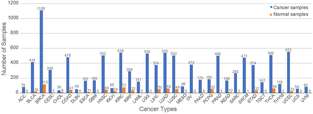
Figure 1. The distribution of the samples for each tumor group. The samples are separated from cancerous and normal tissue samples.

The 56,716 genes' expression levels are in the log₂(FPKM+1) unit where FPKM is the number of fragments per kilobase per million mapped reads. To reduce the complexity of the model, a total of 7,091 most informative genes were selected, which had a mean expression level >0.5 and a standard deviation >0.8. We standardized the gene expression between 0 and 1 in this study to ensure the convergence of the model.

Graph Generated by Co-expressions

Two different input graphs were generated, a co-expression graph and a PPI graph from the STRING database (https://string-db.org/) [22, 23]. To create the co-expression graph, Spearman correlation was calculated using MATLAB (Mathworks Inc., MA) to generate a correlation matrix between each gene in the dataset. Spearman Correlation is a widely adopted method to assess monotonic linear or non-linear relationships in sequencing data [26]. If the correlation between two genes is >0.6 with a p < 0.05, a weight of 1 is placed in an adjacency matrix, otherwise 0. If there is no correlation >0.6 with a given gene, then that gene is removed from the gene list, leading to a total of 3,866 genes in the co-expression graph. The graph structure is represented by a 3,866 by 3,866 adjacency matrix, W_co−expr.

Graph Generated by PPI Database

All 7,091 genes were fed into the BioMart databased to find the corresponding unique Ensembl protein IDs [27]. All human protein interactions were downloaded from the STRING website [22, 23]. Due to the existence of non-coding genes in the TCGA dataset and a limited amount of proteins in the STRING database, a total of 4,444 genes were selected to build the graph. Connections among the genes with medium confidence in the STRING database were considered. If a connection between two genes is considered, a weight of 1 will be placed in an adjacency matrix. The PPI graph is represented by a 4,444 by 4,444 adjacency matrix, W_PPI. The string database is selected for the PPI interactions due to the quantity and quality of data coverage, convenient visualization support, and user-friendly file exchange format [28].

Graph Generated by Singleton Nodes

All 7,091 genes were used in PPI and singleton node graph where all 2,647 genes not included in the PPI graph were treated as singleton nodes. The 7,091 by 7,091 adjacency matrix included the 4,444 by 4,444 adjacency matrix W_PPI from the PPI graph at the upper-left corner and zeros in other places. The same occurs in the co-expression and singleton graph. The additional 3,225 genes that are not included in the co-expression graph are included as singleton nodes where W_co−expr upper-left corner and zeros in other places to generate a 7,091 by 7,091 adjacency matrix.

Proposed GCNN Models

The GCNN includes an input graph represented by the adjacency matrix, graph convolutional layer (coarsening and pooling), and a hidden layer fully connected to a softmax output layer as shown in Figure 2. We trained four different ChebNet based on the co-expression, co-expression+singleton, PPI, and PPI+singleton networks.

FIGURE 2

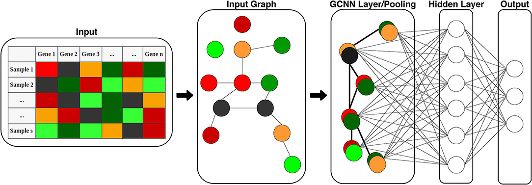
Figure 2. Structure of the proposed GCNN model. The model includes two parts: graph convolution and a fully connected output layer for classification. Input is 1D gene expression levels of TCGA samples and the adjacency matrix of genes (input graph). The graph is then pooled into a single GCNN layer to be fed into the hidden and output layers.

Background on ChebNet

ChebNet is a computationally efficient implementation of GCNN, which approximates the computationally complex global filter on the graph by fast localized filters by using Chebyshev's polynomials. To explain ChebNet for our problem, consider that the gene expression data, x ∈ Rⁿ can be mapped to a graph, G = (V, E) where V is a list of vertices or nodes, E is a list of edges between the nodes, and n denotes the number of gene/nodes. The adjacency matrices generated previously were used to encode the connections, i.e., the edge weights between vertices. Let W = (w_ij) ∈ R ^{n × n} represent the matrix of edge weights and the graph Laplacian of W can express as

$\begin{array}{ll}L=I_n-D^{-\frac{1}{2}}W{D}^{-\frac{1}{2}},\text{L}\in {\text{R}}^{\text{nxn}}& (1)\end{array}$

where D is the diagonal matrix with D_ii = $\sum _j{w}_{ij}$, and I_n is an n × n identity matrix. The graph Laplacian L is a self-adjoint positive-semidefinite operator and therefore allows an eigendecomposition L = UΛU^T, where U=[u₁, u₂, …, u_n] represents n eigenvectors of L and Λ= diag[λ₁, λ₂, …, λ_n] is a diagonal matrix composed of the eigenvalues of L [29]. Such decomposition admits a spectral-domain operation similar to the Fourier transform in the Euclidean. Application of a filter G to the input signal x on the graph can be calculated by the convolution of G and x, which can be computed in the spectral domain according to in the following equation,

$\begin{array}{ll}\text{y }=g(\text{L})\text{x }=g\left(\text{U}\Lambda {\text{U}}^T\right)\text{x }=\text{U}g(\Lambda ){\text{U}}^T\text{x},& (2)\end{array}$

where g_θ is the spectral representation of the filter that gets increasingly complex with the dimension of the input data and the number of neighboring nodes.

To reduce the complexity, a polynomial expansion of g can be obtained as

$\begin{array}{ll}{g}_{\theta }(\Lambda )={\sum }_{k=0}^{K-1}{\theta }_k{\Lambda }_k,& (3)\end{array}$

where ${\Lambda }_k=\mathrm{\text{diag}}\left[{\lambda }_1^k,{\lambda }_2^k,\dots ,{\lambda }_n^k\right]$and θ_k are the polynomial coefficients. It is shown [29] that this expansion yields local filters with manageable computation. A Chebyshev approximation T_m(x) of order m have been proposed in Defferrard et al. for this expansion and is represented by

$\begin{array}{ll}{T}_m(x)=2x{T}_{m-1}(x)-T_{m-2}(x),& (4)\end{array}$

where T₀ (x) = 1 and T₁(x) = x [29, 30]. Then, the local filter described in (3) can be expressed as

$\begin{array}{ll}{g}_{\theta }(\Lambda )={\sum }_{k=0}^{K-1}{\theta }_k{\text{T}}_k(\hat{\Lambda }),& (5)\end{array}$

where $\hat{\Lambda }$ is a scaled Λ defined fas

$\begin{array}{ll}\hat{\Lambda }==2\Lambda /{\lambda }_{max}-I_n,& (6)\end{array}$

that maps the eigenvalues in [−1,1]. This makes the Chebyshev expansion to have ${\hat{x}}_0$ =x and ${\hat{x}}_1=\hat{L}x$ which greatly decreases the computational cost. This resulting implementation is called ChebNet.

Graph Convolutional Network

Kipf et al. further simplified this ChebNet by keeping the filter to be an order of 1 and set θ = θ₀ = −θ₁ to prevent overfitting. This reduced (2) into [18]

$\begin{array}{ll}\text{y}=\theta \left(I_n+D^{-\frac{1}{2}}W{D}^{-\frac{1}{2}}\right)x.& (7)\end{array}$

A normalization with $\hat{W}=W+1$ and ${\hat{D}}_{ii}=\sum _j{\hat{W}}_{ij}$ is applied that leads to the final expression for the filtering as

$\begin{array}{ll}y=\theta \left({\hat{D}}^{-\frac{1}{2}}\hat{W}{\hat{D}}^{-\frac{1}{2}}\right)x& (8)\end{array}$

This resulting implementation is also referred to as graph convolutional network (GCN).

Coarsening, Pooling, and Output Layer

A greedy algorithm was used for layer coarsening, which reduced the number of nodes roughly by half. The greedy rule chose an unselected node to be paired with another unpaired neighbor node and their vertices being summed together. When pooling and coarsening a singleton node, the node grouped with a random node that was unpaired.

The output nodes of the final GCNN layer served as the input to a single dense fully connected layer with a ReLu function which then led to the output layer with a softmax function to get the probabilities.

Loss Function, Optimization, and Hyperparameter Selection

Categorical cross-entropy was used as the loss function and the Adam optimizer was selected for all four GCNN models. Random Search was used to find the optimal pooling, learning rate, size of the hidden layer, and batch size. The hyperparameters were selected based on the highest accuracy and lowest loss function with multiple model parameters providing similar results. The parameters chosen remained consistent throughout the four models. The epoch and batch size was chosen as 20 and 200, respectively. Only one coarsened GCNN layer was used with 1 filter, an average pooling of 2, and one hidden layer was selected after the GCNN layer of 1,024 nodes. The only hyperparameter that changed was the learning rate which increased from 0.001 to 0.005 in the singleton graphs. 5-fold cross-validation was used to train and test the model.

Computational Gene Perturbation Post-modeling Analysis of GCNN Model

Determining the most influential gene to each cancer type or normal tissue classification is an important task for model analysis and verification, yet very difficult for the GCNN model due to the collapse of nodes in the graph. Inspired by Ahn's model analysis for a single type of cancer, a computational gene perturbation analysis for multiple cancer classes was used in this study [12]. The pseudocode is shown in Figure 3. The gene perturbation post-modeling analysis examined how much the predictions of a trained model changed before and after a gene was perturbed in computer simulations, where significant prediction accuracy change suggested the importance of the gene in the classification.

Step 1: Screen samples

FIGURE 3

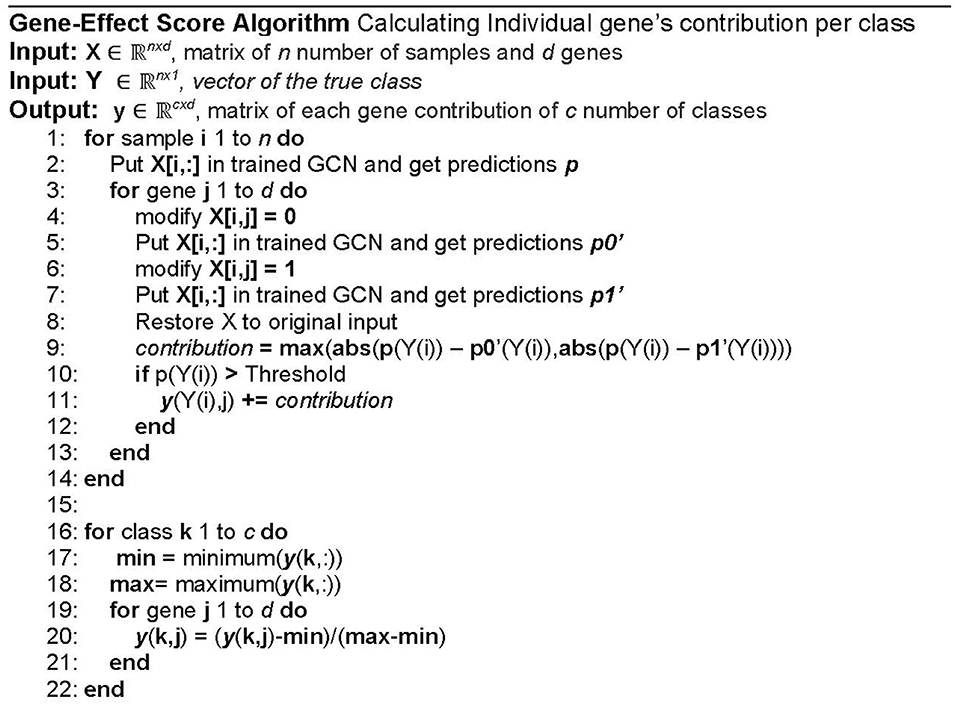
Figure 3. The pseudocode for the in silico gene perturbation post-modeling analysis.

A sample without a satisfactory prediction (>0.5) given by the GCNN model was removed from this analysis since it did not represent the class adequately. A threshold of 0.5 was chosen since any prediction greater than that guaranteed that classification.

Step 2: Calculate the contribution score of each gene to 34 classification types

In the perturbation post-modeling analysis, each gene was set to the lowest value (0) and then the highest value (1) at a time to see how the expression change would affect the prediction accuracy of the trained model for each sample after the screening. The newly obtained prediction accuracies caused by a gene were compared to the original prediction accuracy from the model for the cancer type labeled by TCGA data. The larger prediction accuracy change of the labeled cancer type was chosen as a contribution score of that gene for that cancer type. The process was repeated for each gene in all cancer types and normal samples, resulting in a contribution score for each gene of all 34 classification groups (33 for cancer types and normal type). The contribution scores were represented by a matrix with dimensions of the number of classes (34) by the number of genes.

Step 3: Normalization

The final contributions were normalized to their respective class resulting in their gene-effect score between 0 (lowest effect) to 1 (highest effect). The normalization was done to standardize the score onto the same scale because some tumor types have more samples thus having more contributions to that class. Min-max normalization was chosen since we only cared for the magnitude, not the direction in which the prediction changes—positively (higher confidence) or negatively (lower confidence). Min–max normalization equation is also shown in the pseudocode as shown in Figure 3. An additional class was added to investigate genes that may be associated with multiple cancer types. A summary statistic termed “Overall Cancer” was calculated by adding the gene-effect scores from all 34 cancer types resulting in scores between 0 and 34.

Results

All of the four models were implemented with Google's TensorFlow package 1.14.1 in python and all codes are available at https://github.com/RicardoRamirez2020/GCN_Cancer.

Accuracy of Predicting Cancer Types

Inputs for co-expression, co-expression+singleton, PPI, and PPI+singleton GCNN are 3,866 by 1, 7,091 by 1, 4,444 by 1, and 7,091 by 1 vectors, respectively. The property of the four graphs and the key hyperparameters for four GCNN models based on the graphs are all shown in Table 1. Though the co-expression graph has fewer nodes, it contains more links than the PPI based graphs, suggesting possible long convergence time.

TABLE 1

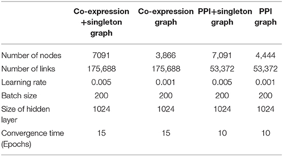
Table 1. Property of four graphs established and the hyperparameters for four GCNN models trained by combined tumor and normal samples.

The prediction accuracy of each GCNN model is shown in Table 2. The PPI+singleton GCNN model performed the best on average and peak values of accuracy. In addition, it was the most stable with the lowest standard deviation as shown in Table 2.

TABLE 2

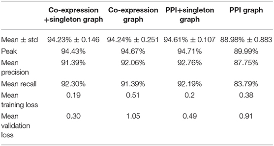
Table 2. Performance of predicting cancer types of four GCNN models trained by combined tumor and normal samples.

The four GCNN models were trained with a combined 11,071 tumor and non-tumor samples initially. To evaluate the training procedure and their robustness against overfitting, we examined loss functions for four models as shown in Supplement 1 using 5-fold cross-validation for training and validation. The validation loss of PPI+singleton GCNN converged to a value <0.5 after 5 epochs with no obvious overfitting (Supplements 1G,H). The co-expression GCNN model demonstrated a similar convergence speed as the PPI+singleton model while having a little higher loss (Supplements 1A,B) and its singleton counterpart having similar convergence speed but a lower loss (Supplements 1C,D). The PPI GCNN model had the longest convergence time but lowest validation loss (>0.5) among the four models (Supplements 1E,F).

The prediction accuracy of the PPI GCNN model was the lowest (88.98% ± 0.88%, mean ± std)% as shown in Table 2. The PPI graph only included genes that were mappable to proteins and have interactions based on the STRING database. Therefore, non-coding genes were not included in the PPI graph. In addition, the protein interaction network might not capture all gene regulations and activities at the transcriptomic level, which might be an explanation of the low performance of the PPI GCNN model. Similarly, another recent PPI based GCNN model for breast cancer subtype classification reported a prediction accuracy of 85%, suggesting the PPI graph itself may not be a complete graph representation for gene expression profiles from TCGA [24]. The GCNN model with the PPI+singleton graph included all the 7,091 genes and demonstrated a >5% increase in prediction accuracy compared with the PPI graph with a smaller accuracy variation as shown in Table 2, suggesting that the additional 2,647 genes could be important in determining cancer type.

Prediction accuracy of the co-expression GCNN model (94.24% ± 0.25%) is comparable to the PPI+singleton GCNN model (94.61% ± 0.11%) and both were better than the PPI GCNN model. While adding singleton nodes helped the PPI graph to achieve better classification, the co-expression graph with singleton nodes did not show a similar effect. GCNN model based on co-expression + singleton graph and co-expression graph demonstrated similar results. This might partially be due to the fact that the PPI network only included 4,444 protein-coding genes from 7,091 selected genes in this study. Adding singleton nodes to PPI brought back the role of non-coding genes that were not in the STRING database and thus improved the performance. In the co-expression graph, 2,315 genes were part of the PPI network, and 1,551 were other genes not inside the PPI network, probably included non-coding genes, which provided additional classification accuracy and robustness. Surprisingly, singleton nodes represented genes not passing the co-expression test and did not have a major impact on the cancer type classification, alluding that transcriptomic regulations between genes and their differential activities played a critical and sufficient role in cancer type prediction. The common genes in both singleton, PPI, and co-expression graphs are shown in Figure 4.

FIGURE 4

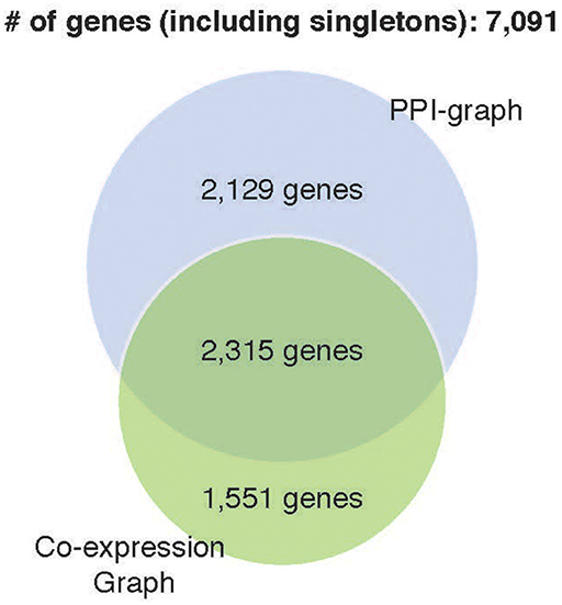
Figure 4. Venn diagram of genes included in four GCNN models. Both singleton graphs contain 7,091 genes. The PPI graph contains 4,444 from the 7,091 genes. The co-expression graph contains 3,866 from the 7,091 genes. The intersection of the PPI graph and the co-expression graph is 2,315 genes.

Further evaluation of micro-averaged precision-recall statistics of the co-expression and co-expression+singleton GCNN models with 34 output classes yielded very interesting observations shown in Figures 5, 6. The largest discrepancy in the precision-recall value appeared for tumor type rectum adenocarcinoma (READ) in all four models. This is due to a large number of READ samples were misclassified into COAD (colon adenocarcinoma), causing a much higher recall level. A total of 68, 16, 95.2, and 72.9%, out of 166 READ samples were classified into COAD cancer type by the co-expression, co-expression+singleton, PPI, and PPI+singleton GCNN model respectively (confusion matrices in Figures 7, 8, and further illustrated in Supplements 2–5). Meanwhile, 6.9, 30.9, 0.2, and 6.4% of 478 COAD samples are misclassified into READ types. Adenocarcinomas of colon or rectum (a passageway connects the colon to anus) are two cancers having different staging procedures, and subsequent treatment, while different molecular aberrations were identified for both of them [31], the overall expression profiles of READ and COAD are similar, probably lead to the higher misclassification. The much more tumor samples in COAD group (n = 478) vs. 166 in READ resulted in model training to bias toward a classification of colon adenocarcinoma when confusion occurred, rather than to rectal adenocarcinoma.

FIGURE 5

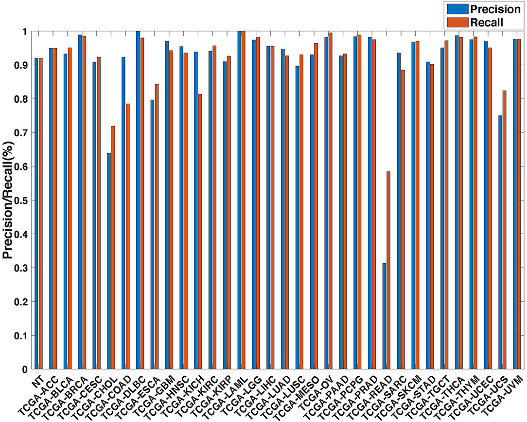
Figure 5. Precision (blue) and recall (red) of the co-expression GCNN models trained with combined 33 different cancer types and normal samples.

FIGURE 6

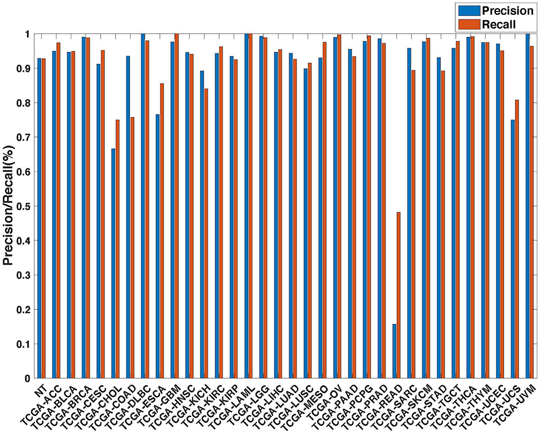
Figure 6. Precision (blue) and recall (red) of the co-expression+singleton GCNN models trained with combined 33 different cancer types and normal samples.

FIGURE 7

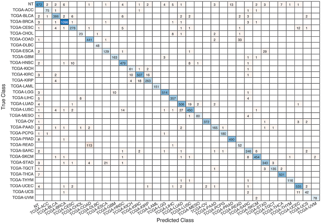
Figure 7. Confusion matrix of all samples predicted by the co-expression GCNN model with combined 33 different cancer types and normal samples.

FIGURE 8

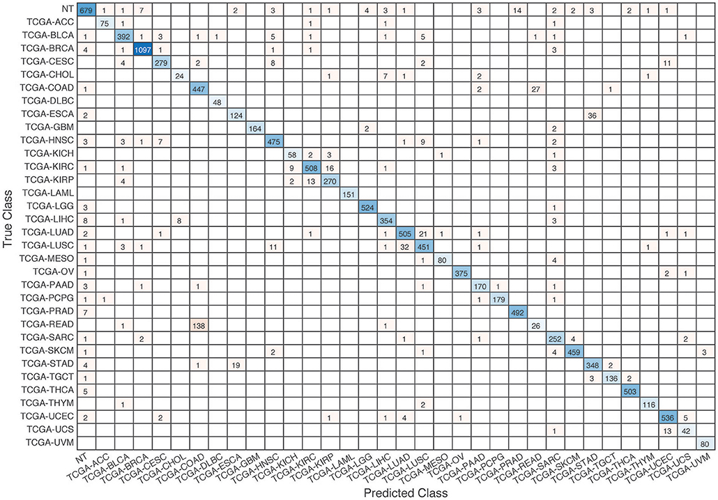
Figure 8. Confusion matrix of all samples predicted by the coexpression+singleton GCNN model with combined 33 different cancer types and normal samples.

Similarly, cholangiocarcinoma (CHOL), a type of liver cancer that forms in the bile duct, has only 36 tumor samples, while 22.2, 22.2, 19.4, and 13.9% of the 36 samples were misclassified into hepatocellular carcinoma (LIHC) by the co-expression, co-expression+singleton, PPI, and PPI+singleton model, respectively. Since cholangiocarcinoma can affect any area of bile ducts, either inside or outside the liver, it is often mixed with both cancerous tissues, thus difficult to separate these two types of cancer. Among 4 models, the PPI+singleton GCNN models performed pretty well to separate these two types of liver cancer with an accuracy of 72% for CHOL and 95% for LIHC, and the co-expression graph resulted in 34% for CHOL and 94.4% for LIHC (Supplement 5 and Figure 7).

Lastly, Uterine carcinosarcoma (UCS) had only 56 tumor samples, frequently confused with the uterine corpus endometrioid carcinoma (UCEC), two types of uterine cancers collected in the TCGA cohort.

UCS classification performed poorly (misclassification rate of 25, 25, 58.9, and 21.4% for co-expression, co-expression+singleton, PPI model, and PPI+singleton GCNN model, respectively), and most of these misclassified samples were in UCEC as expected. We also noted that there were no normal tissues collected within UCS type, the GCNN model might not learn to remove tissue-specific markers.

Not all samples from the same organ classified together. There are three types of kidney cancers, kidney chromophobe (KICH), kidney clear cell carcinoma (KIRC), and kidney papillary cell carcinoma (KIRP) in the TCGA dataset, and two lung cancers, lung adenocarcinoma (LUAD) and lung squamous cell carcinoma (LUSC) in the TCGA cohort. The co-expression GCNN model classified KICH, KIRC, KIRP, LUAD, and LUSC with accuracy rates at 93.8, 94, 91, 94.6, and 89.6%, while the PPI+singleton model has the accuracy at 90.7, 94.6, 93.8, 95.3, and 91.2%. Other GCNN models have comparable performance.

Cancer-Specific Classification

Previous studies have demonstrated promising classification results on TCGA data. Hoadley et al. have identified 28 distinct molecular subtypes arising from the 33 different tumor types analyzed across at least four different TCGA platforms including chromosome-arm-level aneuploidy, DNA hypermethylation, mRNA, and miRNA expression levels and reverse-phase protein arrays [32]. Their results illustrated significant molecular similarities among anatomically related cancer types. Meanwhile, other recent studies have demonstrated the successful classification of cancer types using either clustering or deep learning algorithms [10, 13]. However, these studies did not include normal samples in the classification and there remained a doubt on whether these classifications were tissue-specific or cancer-specific. Anh and our group have recently reported the classification of the tumor and normal tissues that suggest possible cancer-specific classification [12, 15].

To verify the cancer-specific classification of the GCNN algorithm, the co-expression GCNN model was used to separate all 1,221 breast tissue samples from the TCGA dataset, among which 113 were normal samples and 1,108 were cancerous. The result showed a mean accuracy of (99.34% ± 0.47%) using 5-fold cross-validation. Overall, about 92% (672 out of 731) normal tissues classified correctly into NT groups, regardless of their origins, suggesting the GCNN models identify cancer-specific samples' class designation without using biomarkers related to specific tissues.

Post-modeling Analysis

Post-modeling analysis of the co-expression GCNN was performed for two reasons. There was no significant difference in accuracy between the coexpression graph and either the PPI+singleton or coexpression+singleton graph. In addition, in silico gene perturbation in a combined co-expression + singleton graph heavily favored singleton nodes, while connected nodes would be compensated by its connected neighbors. Therefore, considering the PPI graph's worst classification performance, the post-modeling analysis was performed on the co-expression GCNN.

A total of 428 potential markers found in the 34 classes with a gene-effect score ≥0.3 (see Methods section), giving an average of approximately 38 genes per class. None of the 428 genes are unique to one specific class, indicating that the co-expression GCNN model relied on the combinations of genes to perform the cancer type classification. The threshold for the gene-effect score of 0.3 was selected based on their histogram of all gene-effect scores (Supplement 6). Thymoma (THYM), testicular germ cell tumors (TGCT), glioblastoma multiforme (GBM), and cervical cancer (CESC) has <10 marker genes with their gene-effect scores >0.3, while mesothelioma (MESO), sarcoma (SARC), and skin cutaneous melanoma (SKCM) had the largest number of genes (>100)s affecting the prediction accuracy in the co-expression GCNN model as shown in Figure 9.

FIGURE 9

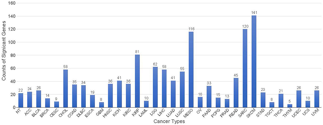
Figure 9. The number of genes significantly affect each cancer type classification with a gene-effect score >0.3.

The top 20 genes selected for breast cancer and the top 20 “Overall Cancer” summary statistics were shown in Table 3. The features learned in breast cancer were interesting: the first 9 genes were Y chromosome related, suggesting that the network learned gender feature first since TCGA breast cancer were obtained all from females. The 11 remaining genes were reported in breast cancer studies, however, whether their functions were actually learned by the GCNN model were yet to be discovered. Genes from the “Overall Cancer” column are those effective in multiple cancer classification.

TABLE 3

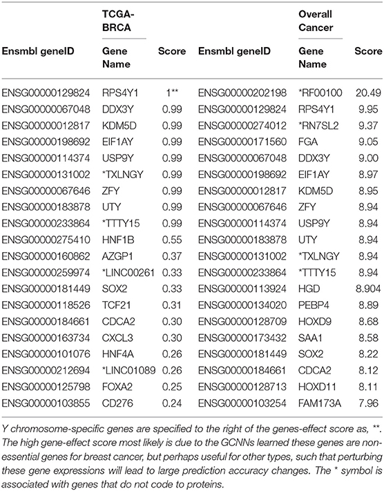
Table 3. Top 20 Genes in Breast Cancer and Overall Cancer Scores.

Discussion

This is the first study to establish a data-driven model for cancer type classification using a graph convolutional neural network approach. The proposed method successfully integrated four different graphs into the deep learning framework. The models were trained by gene expressions from the entire TCGA collections and achieved cancer type prediction accuracy at 94.6%, which is better than or comparable to other machine learning algorithms previously reported [10, 13, 15]. Our GCNN model successfully integrated normal and tumor samples together to further enrich for cancer-specific prediction. Our unique implementation of model interpretation is also novel, where an in silico gene perturbation procedure was executed to evaluate the role of each gene in classification through a novel gene-effect scoring method.

In the study presented here, a total of 7,091 genes from the complete TCGA dataset were chosen with a mean >0.5 and a standard deviation >0.8. Obviously, changing the threshold on mean and standard deviation could generate different numbers of genes to be selected. Our earlier deep learning studies suggested that genes selected captured sufficient information for the proposed objectives [15, 33], however, the sensitivity of the chosen threshold for the GCNN models may require further investigation. The graph complexity was also tested with similarly, multiple different correlations thresholds to generate co-expression graphs. Correlation of 0.6 with a p < 0.05 gave the best results, the model had a sufficient number of discriminative genes to classify each cancer type but not overly generalized where the Laplacian of the graph lost its significant meaning. Meanwhile, if the correlation threshold is too high, some discriminative genes may be excluded from the graph. Though it might be computationally costly, these thresholds can be included as learning parameters in our future studies.

FPKM unit was used in this study because it is one of the normalized measures available from the TCGA data portal (GDC) and it is widely used in official TCGA publications. Another gene expression unit, TPM, or transcriptions per million, is another measure of gene abundance potentially with higher consistency among samples. We downloaded TPM data from the UCSC TumorMap and compared it to the FPKM dataset used in the present study. Among the 6,583 genes and 9,617 samples common between the two datasets (total numbers in our manuscript, 7,091 genes, and 11,071 samples), TPM and FPKM values were greatly consistent (Pearson correlation coefficient, 0.94). Furthermore, 84.8 and 94.1% of the edges in the coexpression network built using FPKM (correlation > 0.6 in FPKM) remained to be highly correlated with correlations >0.6 and 0.5, respectively, in the TPM dataset. A total of 86.1% of genes remained in the coexpression network constructed in the TPM dataset with an identical threshold of correlation >0.6. Thus, we expect the coexpression network and GCNN performance achieved using the TPM dataset to be very similar to FKPM.

The co-expression graph generated using correlation coefficients captures linear regulation relationships predominantly. The mutual information (MI) method including ARACNe and MINDY may serve as an alternative to correlation-based methods to measure gene interactions, especially non-linear relationships [34, 35]. However, due to a requirement of permutations for each gene pair to assess statistical significance, MI consumes tremendously more computation capacity than correlation and thus is hardly possible for a genome-wide search. Therefore, the most successful applications of MI methods are mainly limited to small pre-defined networks, such as transcript factor bindings and miRNA targets (known as the ceRNA regulation). In our previous papers, we compared the two types of methods and showed that correlation-based methods achieved higher performance and efficiency in capturing the dynamic gene regulations using gene expression data [36, 37]. Furthermore, it was reported that gene regulation is typically linear or monotonic and thus correlation-based methods can achieve equivalent or even better performance [38]. Thus, to enable our GCNN model to a genome-wide network that incorporated as much information as possible, we utilized correlation to construct co-expression networks.

In the PPI+singleton GCNN model, isolated genes, such as non-coding genes, are integrated as singleton nodes in the graph. Since these singleton genes may have higher gene-effect scores than the coding genes (2,674 genes are not in PPI-graph), databases for non-coding genes, RNA-RNA interaction, and transcription factors should be considered to establish links between these genes and genes inside the PPI graph for a complete GCNN model. Another possible approach to build a graph for a GCNN model is a literature-derived graph. There are over 4 million cancer-related manuscripts in the PubMed database and building a literature-derived graph will be time-consuming and therefore is not included in this study. Previously, we established a knowledge map of post-myocardial infarction responses by automatically text-mining more than 1 million abstracts from PubMed [39]. We will use literature review tools to build a literature-derived network for cancer study in our future research. One thing worth mentioning is that the deep-learning algorithm is purely a data-driven method and some techniques to integrate biological meaning to the graph-related network may require an overhaul of our current GCNN model design, such as the development of a GCNN model based on the latest results of explainable networks [40, 41].

Data Availability Statement

Publicly available datasets were analyzed in this study. This data can be found here: https://bioconductor.org/packages/release/bioc/html/TCGAbiolinks.html.

Author Contributions

RR and Y-FJ designed the research. RR performed the GCNN algorithm. RR, Y-CC, MM, JR, and AH processed the data and validation. RR, Y-FJ, YH, and YC analyzed the results and drafted the manuscript. All authors contributed to the article and approved the submitted version.

Funding

NCI Cancer Center Shared Resources (NIH-NCI P30CA054174 to YC), NIH (CTSA UL1TR002645 to YC, R01GM113245 to YH, and K99CA248944 to Y-CC), CPRIT (RP160732 to YC, RP190346 to YC and YH), San Antonio Life Science Institute (SALSI Postdoctoral Research Fellowship 2018 to Y-CC), and the Fund for Innovation in Cancer Informatics (ICI Fund to Y-CC and YC).

Conflict of Interest

The authors declare that the research was conducted in the absence of any commercial or financial relationships that could be construed as a potential conflict of interest.

Acknowledgments

The authors acknowledge the support from Valero Scholarship for RR during the past 3 years.

Supplementary Material

The Supplementary Material for this article can be found online at: https://www.frontiersin.org/articles/10.3389/fphy.2020.00203/full#supplementary-material

References

1. Siegel RL, Miller KD, Jemal A. Cancer statistics, 2019. CA Cancer J Clin. (2019) 69:7–34. doi: 10.3322/caac.21551

CrossRef Full Text | Google Scholar

2. Barry MJ. Prostate-specific–antigen testing for early diagnosis of prostate cancer. N Engl J Med. (2001) 344:1373–7. doi: 10.1056/NEJM200105033441806

PubMed Abstract | CrossRef Full Text | Google Scholar

3. Boyle P, Ferlay J. Mortality and survival in breast and colorectal cancer. Nat Clin Pract Oncol. (2005) 2:424. doi: 10.1038/ncponc0288

PubMed Abstract | CrossRef Full Text | Google Scholar

4. Brett G. Earlier diagnosis and survival in lung cancer. Br Med J. (1969) 4:260–2. doi: 10.1136/bmj.4.5678.260

PubMed Abstract | CrossRef Full Text | Google Scholar

5. McPhail S, Johnson S, Greenberg D, Peake M, Rous B. Stage at diagnosis and early mortality from cancer in England. Br J Cancer. (2015) 112:S108. doi: 10.1038/bjc.2015.49

PubMed Abstract | CrossRef Full Text | Google Scholar

6. Kourou K, Exarchos TP, Exarchos KP, Karamouzis MV, Fotiadis DI. Machine learning applications in cancer prognosis and prediction. Comput Struct Biotechnol J. (2015) 13:8–17. doi: 10.1016/j.csbj.2014.11.005

PubMed Abstract | CrossRef Full Text | Google Scholar

7. Statnikov A, Wang L, Aliferis CF. A comprehensive comparison of random forests and support vector machines for microarray-based cancer classification. BMC Bioinformatics. (2008) 9:319. doi: 10.1186/1471-2105-9-319

PubMed Abstract | CrossRef Full Text | Google Scholar

8. Cruz JA, Wishart DS. Applications of machine learning in cancer prediction and prognosis. Cancer Informat. (2006) 2:117693510600200030. doi: 10.1177/117693510600200030

PubMed Abstract | CrossRef Full Text | Google Scholar

9. Liu JJ, Cutler G, Li W, Pan Z, Peng S, Hoey T, et al. Multiclass cancer classification and biomarker discovery using GA-based algorithms. Bioinformatics. (2005) 21:2691–7. doi: 10.1093/bioinformatics/bti419

PubMed Abstract | CrossRef Full Text | Google Scholar

10. Li Y, Kang K, Krahn JM, Croutwater N, Lee K, Umbach DM, et al. A comprehensive genomic pan-cancer classification using The Cancer Genome Atlas gene expression data. BMC Genomics. (2017) 18:508. doi: 10.1186/s12864-017-3906-0

PubMed Abstract | CrossRef Full Text | Google Scholar

11. Holzinger A, Kieseberg P, Weippl E, Tjoa AM. Current advances, trends and challenges of machine learning and knowledge extraction: from machine learning to explainable AI. In: Holzinger A, Kieseberg P, Tjoa AM, Weippl E, editors. Machine Learning and Knowledge Extraction. Cham: Springer International Publishing (2018). p. 1–8.

Google Scholar

12. Ahn T, Goo T, Lee C, Kim S, Han K, Park S, et al. Deep learning-based identification of cancer or normal tissue using gene expression data. In: 2018 IEEE International Conference on Bioinformatics and Biomedicine (BIBM). Madrid (2018). p. 1748–52.

Google Scholar

13. Lyu B, Haque A. Deep learning based tumor type classification using gene expression data. bioRxiv. (2018) 364323. doi: 10.1101/364323

CrossRef Full Text | Google Scholar

14. Chen H.-I, Chiu Y.-C, Zhang T, Zhang S, Huang Y, Chen Y. GSAE: an autoencoder with embedded gene-set nodes for genomics functional characterization. BMC Syst Biol. (2018) 12:142. doi: 10.1186/s12918-018-0642-2

PubMed Abstract | CrossRef Full Text | Google Scholar

15. Mostavi M, Chiu Y.-C, Huang Y, Chen Y. Convolutional neural network models for cancer type prediction based on gene expression. BMC Med Genomics. (2020) 13:1–13. doi: 10.1186/s12920-020-0677-2

PubMed Abstract | CrossRef Full Text | Google Scholar

16. Bronstein MM, Bruna J, LeCun Y, Szlam A, Vandergheynst P. Geometric deep learning: going beyond euclidean data. IEEE Signal Proc Mag. (2017) 34:18–42. doi: 10.1109/MSP.2017.2693418

CrossRef Full Text | Google Scholar

17. Hamilton W, Ying Z, Leskovec J. Inductive representation learning on large graphs. Adv Neural Inform Proc Syst. (2017) 1024–34.

Google Scholar

18. Kipf TN, Welling M. Semi-supervised classification with graph convolutional networks. arXiv preprint arXiv:1609.02907 (2016).

Google Scholar

19. Sanchez-Gonzalez A, Heess N, Springenberg JT, Merel J, Riedmiller M, Hadsell R, et al. Graph networks as learnable physics engines for inference and control. arXiv preprint arXiv:1806.01242 (2018).

Google Scholar

20. Battaglia P, Pascanu R, Lai M, Rezende DJ. Interaction networks for learning about objects, relations and physics. Adv Neural Inform Proc Syst. (2016) 4502–10.

Google Scholar

21. Chereda H, Bleckmann A, Kramer F, Leha A, Beissbarth T. Utilizing molecular network information via graph convolutional neural networks to predict metastatic event in breast cancer. Stud Health Technol Inform. (2019) 267:181–6. doi: 10.3233/SHTI190824

PubMed Abstract | CrossRef Full Text | Google Scholar

22. Szklarczyk D, Morris JH, Cook H, Kuhn M, Wyder S, Simonovic M, et al. The STRING database in 2017: quality-controlled protein-protein association networks, made broadly accessible. Nucleic Acids Res. (2017) 45:D362–8. doi: 10.1093/nar/gkw937

PubMed Abstract | CrossRef Full Text | Google Scholar

23. Szklarczyk D, Franceschini A, Wyder S, Forslund K, Heller D, Huerta-Cepas J, et al. STRING v10: protein–protein interaction networks, integrated over the tree of life. Nucleic Acids Res. (2014) 43:D447–52. doi: 10.1093/nar/gku1003

PubMed Abstract | CrossRef Full Text | Google Scholar

24. Rhee S, Seo S, Kim S. Hybrid approach of relation network and localized graph convolutional filtering for breast cancer subtype classification. arXiv preprint arXiv:1711.05859 (2017). doi: 10.24963/ijcai.2018/490

CrossRef Full Text | Google Scholar

25. Colaprico A, Silva TC, Olsen C, Garofano L, Cava C, Garolini D, et al. TCGAbiolinks: an R/Bioconductor package for integrative analysis of TCGA data. Nucleic Acids Res. (2015) 44:e71. doi: 10.1093/nar/gkv1507

PubMed Abstract | CrossRef Full Text | Google Scholar

26. Siska C, Kechris K. Differential correlation for sequencing data. BMC Res Notes. (2017) 10:54. doi: 10.1186/s13104-016-2331-9

PubMed Abstract | CrossRef Full Text | Google Scholar

27. Smedley D, Haider S, Durinck S, Pandini L, Provero P, Allen J, et al. The BioMart community portal: an innovative alternative to large, centralized data repositories. Nucleic Acids Res. (2015) 43:W589–8. doi: 10.1093/nar/gkv350

PubMed Abstract | CrossRef Full Text | Google Scholar

28. Jeanquartier F, Jean-Quartier C, Holzinger A. Integrated web visualizations for protein-protein interaction databases. BMC Bioinformatics. (2015) 16:195. doi: 10.1186/s12859-015-0615-z

PubMed Abstract | CrossRef Full Text | Google Scholar

29. Defferrard M, Bresson X, Vandergheynst P. Convolutional neural networks on graphs with fast localized spectral filtering. Adv Neural Inform Proc Syst. (2016) 3844–52.

Google Scholar

30. Hammond DK, Vandergheynst P, Gribonval R. Wavelets on graphs via spectral graph theory. Appl Comput Harmonic Anal. (2011) 30:129–50. doi: 10.1016/j.acha.2010.04.005

CrossRef Full Text | Google Scholar

31. Li FY, Lai MD. Colorectal cancer, one entity or three. J Zhejiang Univ Sci B. (2009) 10:219–29. doi: 10.1631/jzus.B0820273

CrossRef Full Text | Google Scholar

32. Hoadley KA, Yau C, Hinoue T, Wolf DM, Lazar AJ, Drill E, et al. Cell-of-origin patterns dominate the molecular classification of 10,000 tumors from 33 types of cancer. Cell. (2018) 173:291–304.e6. doi: 10.1016/j.cell.2018.03.022

PubMed Abstract | CrossRef Full Text | Google Scholar

33. Chiu Y.-C, Chen H.-IH, Zhang T, Zhang S, Gorthi A, Wang L.-J, et al. Predicting drug response of tumors from integrated genomic profiles by deep neural networks. BMC Med Genomics. (2019) 12:18. doi: 10.1186/s12920-019-0569-5

CrossRef Full Text | Google Scholar

34. Margolin AA, Nemenman I, Basso K, Wiggins C, Stolovitzky G, Favera RD, et al. ARACNE: an algorithm for the reconstruction of gene regulatory networks in a mammalian cellular context. BMC Bioinformatics. (2006) 7(Suppl. 1):S7. doi: 10.1186/1471-2105-7-S1-S7

PubMed Abstract | CrossRef Full Text | Google Scholar

35. Wang K, Saito M, Bisikirska BC, Alvarez MJ, Lim WK, Rajbhandari P, et al. Genome-wide identification of post-translational modulators of transcription factor activity in human B cells. Nat Biotechnol. (2009) 27:829–39. doi: 10.1038/nbt.1563

PubMed Abstract | CrossRef Full Text | Google Scholar

36. Hsiao TH, Chiu YC, Hsu PY, Lu TP, Lai LC, Tsai MH, et al. Differential network analysis reveals the genome-wide landscape of estrogen receptor modulation in hormonal cancers. Sci Rep. (2016) 6:23035. doi: 10.1038/srep23035

PubMed Abstract | CrossRef Full Text | Google Scholar

37. Chiu Y.-C, Wang L.-J, Lu T.-P, Hsiao T.-H, Chuang EY, Chen Y. Differential correlation analysis of glioblastoma reveals immune ceRNA interactions predictive of patient survival. BMC Bioinformatics. (2017) 18:132. doi: 10.1186/s12859-017-1557-4

PubMed Abstract | CrossRef Full Text | Google Scholar

38. Song L, Langfelder P, Horvath S. Comparison of co-expression measures: mutual information, correlation, and model based indices. BMC Bioinformatics. (2012) 13:328. doi: 10.1186/1471-2105-13-328

PubMed Abstract | CrossRef Full Text | Google Scholar

39. Nguyen NT, Zhang X, Wu C, Lange RA, Chilton RJ, Lindsey ML, et al. Integrative computational and experimental approaches to establish a post-myocardial infarction knowledge map. PLOS Comput Biol. (2014) 10:e1003472. doi: 10.1371/journal.pcbi.1003472

PubMed Abstract | CrossRef Full Text | Google Scholar

40. Holzinger A, Langs G, Denk H, Zatloukal K, Müller H. Causability and explainability of artificial intelligence in medicine. WIREs Data Mining Knowl Discov. (2019) 9:e1312. doi: 10.1002/widm.1312

PubMed Abstract | CrossRef Full Text | Google Scholar

41. Preuer K, Klambauer G, Rippmann F, Hochreiter S, Unterthiner T. Interpretable deep learning in drug discovery. In: Samek W, Montavon G, Vedaldi A, Hansen LK, Müller K.-R, editors. Explainable AI: Interpreting, Explaining and Visualizing Deep Learning. Cham: Springer International Publishing (2019). p. 331–45.

Google Scholar

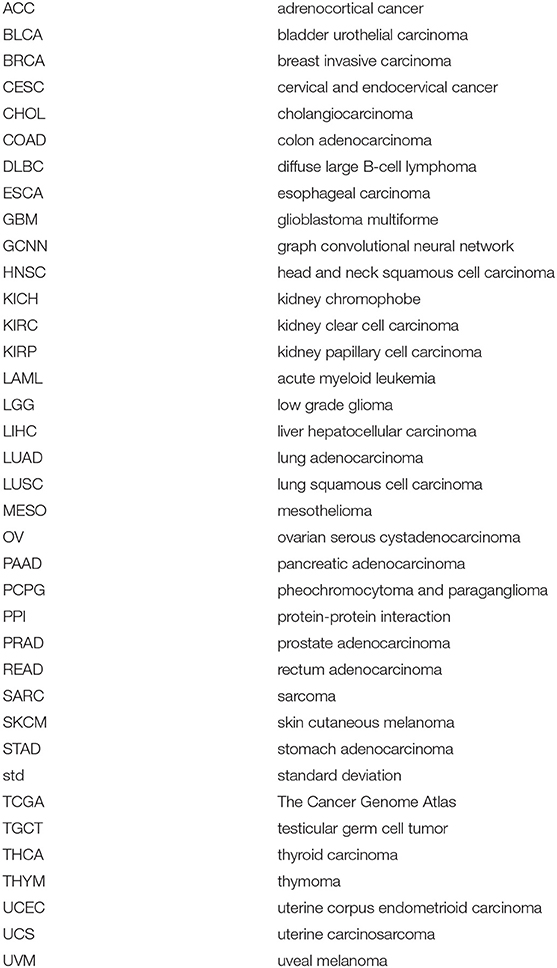
Nomenclature