Muon capture on deuteron using local chiral potentials

1 Introduction

The muon capture on a deuteron, i.e. the process

${\mu }^{-}+d\to n+n+{\nu }_{\mu },(1)$

is one of the few weak nuclear reactions involving light nuclei which, on one side, are experimentally accessible, and, on the other, can be studied using ab initio methods. Furthermore, it is a process closely linked to the proton–proton weak capture, the so-called pp reaction,

$p+p\to d+e^{+}+{\nu }_e,(2)$

which, although being of paramount importance in astrophysics, is not experimentally accessible due to its extremely low rate and can only be calculated. Since the theoretical inputs to study reaction (2) and reaction (1) are essentially the same, the comparison between the experiment and theory for muon capture provides a strong test for the pp studies.

The muon capture reaction (1) can take place in two different hyperfine states, f = 1/2 and 3/2. Since it is well known that the doublet capture rate is about 40 times larger than the quartet one (see, for instance, Ref. [1]), we will consider the f = 1/2 state only, and we will focus on the doublet capture rate, Γ^D. The experimental situation for Γ^D is quite confused, with available measurements which are relatively old. These are the ones of Refs. [2–5], 365 (96) s⁻¹, 445 (60) s⁻¹, 470 (29) s⁻¹, and 409 (40) s⁻¹, respectively. All these data are consistent with each other within the experimental uncertainties, which are, however, quite large. To clarify the situation, an experiment with the aim of measuring Γ^D with 1% accuracy is currently performed at the Paul Scherrer Institute, in Switzerland, by the MuSun Collaboration [6].

Many theoretical studies are available for the muon capture rate Γ^D. A review of the available literature from up to about 10 years ago can be found in Ref. [7]. Here, we focus on the work conducted in the past 10 years. To the best of our knowledge, the capture rate Γ^D has been studied in Refs. [8–12]. The studies of Refs. [9, 11] were performed within the phenomenological approach, using phenomenological potentials and currents. In Ref. [9], the first attempt to use the chiral effective field theory (χEFT) was presented, within the so-called hybrid approach, where a phenomenological nuclear interaction is used in conjunction with χEFT weak nuclear charge and current operators. In the study we present in this contribution, though, we are interested not only in the determination of Γ^D but also an assessment of the theoretical uncertainty. This can be grasped more comfortably and robustly within a consistent χEFT approach. Therefore, we review only the theoretical works of Refs. [8, 10, 12], which were performed within a consistent χEFT. The studies of Refs. [8, 10] were essentially performed in parallel. They both employed the latest (at those times) nuclear chiral potentials and consistent weak current operators. In Ref. [8], the doublet capture rate was found to be Γ^D = 388.1 (4.3) s⁻¹, when the NN chiral potentials of Ref. [13], obtained up to the next-to-next-to-next-to-leading order (N3LO) in the chiral expansion, were used. When only the ${}^{1}S_0$ channel of the final nn scattering state was retained, it was found that ${\mathrm{\Gamma }}^D({}^{1}S_0)=247.7(2.8)$ s⁻¹. In Ref. [10], a simultaneous study of the muon capture on a deuteron and ³He was performed using the same N3LO chiral potentials, but varying the potential cutoff Λ = 500, 600 MeV [13, 14], and consequently refitting consistently for each value of Λ the low-energy constants (LECs) entering into the axial and vector current operators. For the muon capture on a deuteron, it was obtained Γ^D = 399 (3) s⁻¹, the spread accounting for the cutoff sensitivity, as well as uncertainties in the LECs and electroweak radiative corrections. When only the ${}^{1}S_0$ channel is considered, ${\mathrm{\Gamma }}^D({}^{1}S_0)=254.9(1.4)$ s⁻¹, where, in this case, the (small) uncertainty arising from electroweak radiative corrections is not included. In the case of the muon capture on ³He, an excellent agreement with the available extremely accurate experimental datum was found. Although obtained by different groups and with some differences in the axial and vector current operators adopted in the calculations, the results of Refs. [8, 10] for Γ^D and ${\mathrm{\Gamma }}^D({}^{1}S_0)$ should be considered in reasonable agreement. It should be mentioned that in both studies of Refs. [8, 10], a relation between the LEC entering the axial current operator (denoted by d_R) and c_D, one of the two LECs entering the three-nucleon potential (the other one being c_E) was taken from Ref. [15]. Then, the A = 3 binding energies and the Gamow–Teller matrix element of tritium β-decay were used to fix both c_D (and consequently d_R) and c_E for each given potential and cutoff Λ. Unfortunately, the relation between d_R and c_D of Ref. [15] is missing of a factor −1/4, as clearly stated in the Erratum of Ref. [10] (see also the Erratum of Ref. [15]). While the work of Ref. [8] has not yet been revisited, that of Ref. [10] has been corrected, finding very small changes in the final results, which become Γ^D = 398 (3) s⁻¹ and ${\mathrm{\Gamma }}^D({}^{1}S_0)=253.5(1.2)$ s⁻¹.

The most recent and systematic study of reaction (1) in χEFT, even if only retaining the ${}^{1}S_{0}nn$ channel, is that of Ref. [12]. There, ${\mathrm{\Gamma }}^D({}^{1}S_0)$ was calculated using a pool of 42 non-local chiral potentials up to the next-to-next-to-leading order (N2LO), with a regulator cutoff Λ in the range 450–600 MeV and six different energy ranges in the NN scattering database [16]. The consistent axial and vector currents were constructed (with the correct relation between d_R and c_D), and a simultaneous fitting procedure for all the involved LECs was adopted. The final result was found to be ${\mathrm{\Gamma }}^D({}^{1}S_0)=252.8(4.6)(3.9){\mathrm{s}}^{-1}$, in excellent agreement with Ref. [10]. Here, the first error is due to the truncation in the chiral expansion and the second one is due to the uncertainty in the parameterization of the single-nucleon axial form factor (see as follows). Furthermore, in Ref. [17], it has been found that a non-proper treatment of the infrared cutoff when the bound-state wave function is represented in a truncated basis (as in the case of Refs. [9, 10]) can lead to an error of the order of $\sim 1$% in the few-nucleon capture cross sections and astrophysical S-factors (as that of the pp reaction, the case studied in Ref. [17]). Therefore, we believe that it is also important to investigate this issue related to the present muon capture process.

The chiral nuclear potentials involved in all the aforementioned studies are highly non-local and expressed in momentum space. This is less desirable than the r-space in the case of the pp reaction, where the treatment in the momentum space of the Coulomb interaction and the higher-order electromagnetic effects is rather cumbersome. To overcome these difficulties, local chiral potentials expressed in the r-space would be highly desirable. These have been developed only in recent years, as discussed in the recent review of Ref. [18]. These potentials are very accurate and have proven to be extremely successful in describing the structure and dynamics of light and medium-mass nuclei. In particular, we are interested in the work of the models of Ref. [19], the so-called Norfolk potentials, for which, in these years, consistent electromagnetic and weak transition operators have been constructed [20–22]. This local chiral framework has been used to calculate energies [23] and charge radii [24] and various electromagnetic observables in light nuclei, as the charge form factors in A = 6, 12 [24] and the magnetic structure of few-nucleon systems [22]. It has also been used to study weak transitions in light nuclei [25, 26], the muon captures on A = 3, 6 nuclei [27], neutrinoless double β-decay for A = 6, 12 [28] and the β-decay spectra in A = 6 [29], and, finally, the equation of the state of pure neutron matter [30, 31]. However, the use of the Norfolk potentials to study the muon capture on a deuteron and the pp reaction is still lacking. One of the aims of this work is to start this path. Given the fact that ${\mathrm{\Gamma }}^D({}^{1}S_0)$ is the main contribution to Γ^D, and the ${}^{1}S_0$ channel is also the only one of interest for pp fusion [32, 33], we focus our attention only on ${\mathrm{\Gamma }}^D({}^{1}S_0)$. A full calculation of Γ^D, together with the rates for muon capture on A = 3, 6 nuclei, is currently underway. The second aim of the present study is to provide a more robust determination of the theoretical uncertainty than the work of Ref. [10], although probably not as robust as the full work presented in Ref. [12]. However, the procedure we plan to apply in the present work is much simpler and, as shown as follows, with a quite similar outcome. We will consider four sources of uncertainties: 1) the first one is due to model dependence. In this study, the use of the local Norfolk potentials will allow us to take into consideration the uncertainty arising from the cutoff variation, as well as the energy ranges in the NN scattering database up to which the LECs are fitted. In fact, as it will be explained in Section 2.2, we will employ four different versions of the Norfolk potentials, obtained using two different sets of short- and long-range cutoffs, and two different energy ranges, up to 125 MeV or up to 200 MeV, in the NN scattering database. 2) The second source of uncertainty arises from the chiral-order convergence. In principle, this should be investigated by maintaining the same order for potentials and weak nuclear currents. However, at present, the Norfolk potentials, for which weak current operators have been consistently constructed, are those obtained at N3LO. This chiral order is needed to reach good accuracy in the description of the NN systems and of light nuclei. Therefore, it is questionable whether a study of reaction (1) using potentials and currents at a chiral order which does not even reproduce the nuclear systems under consideration, would be of real interest. As a consequence, we will study, in the present work, only the chiral-order convergence for the weak nuclear currents, keeping fixed the chiral order of the adopted potentials. 3) The third source of uncertainty is due to the uncertainty in the parameterization of the single-nucleon axial form factor $g_A(q_{\sigma }^2)$ as a function of the squared four-momentum transfer $q_{\sigma }^2$. This aspect is discussed in detail in Section 2.2. Here, we only notice that the most recent parameterization for the single-nucleon axial form factor is given by

$g_A\left(q_{\sigma }^2\right)=g_A\left(1-\frac{1}{6}{r}_A^2{q}_{\sigma }^2+\cdots \right),(3)$

where the dots indicate higher-order terms, which are typically disregarded, and r_A is the axial charge radius, its square being given by $r_A^2=0.46(16)$ fm² [34]. The large uncertainty on $r_A^2$ will significantly affect the total uncertainty budget, as already found in Ref. [12]. 4) The final source of uncertainty is the one arising from the numerical technique adopted to solve the bound and scattering A = 2 systems. Taking into consideration the arguments of Ref. [17], we have decided to use two methods. The first one is the method already developed by Refs. [9, 10], i.e., a variational method, in which the bound and scattering wave functions are expanded on a known basis and the unknown coefficients of these expansions are obtained using variational principles. The second method is the so-called Numerov method, where the tail of the bound-state wave function is, in fact, imposed “by hand” (see Section 2.3). This last source of uncertainty will be shown to be completely negligible.

The paper is organized as follows: Section 2 presents the theoretical formalism, providing a schematic derivation for ${\mathrm{\Gamma }}^D({}^{1}S_0)$ in Section 2.1, a description of the adopted nuclear potentials and currents in Section 2.2, and a discussion of the methods used to calculate the deuteron and nn wave functions in Section 2.3. The results for ${\mathrm{\Gamma }}^D({}^{1}S_0)$ are presented and discussed in Section 3, and some concluding remarks and an outlook are given in Section 4.

2 Theoretical formalism

We discuss, in this section, the theoretical formalism developed to calculate the muon capture rate. In particular, Section 2.1 gives the main steps of the formalism used to derive the differential and the total muon capture rate on a deuteron in the initial doublet hyperfine state. A through discussion is given by Ref. [9]. Section 2.2 reports the main characteristics of the nuclear potentials and currents we used in the present study. Finally, Section 2.3 presents the variational and the Numerov methods used to calculate the deuteron bound and nn scattering wave functions.

2.1 Observables

The differential capture rate in the doublet initial hyperfine state dΓ^D/dp can be written as [9]

$\frac{d{\mathrm{\Gamma }}^D}{dp}=E_{\nu }^2\left[1-\frac{E_{\nu }}{\left(m_{\mu }+m_d\right)}\right]\frac{p^{2}d\widehat{\mathbf{p}}}{8{\pi }^4}\overline{|T_W{|}^2},(4)$

where p is the nn relative momentum, and

$E_{\nu }=\frac{{\left(m_{\mu }+m_d\right)}^2-4m_n^2-4p^2}{2\left(m_{\mu }+m_d\right)},(5)$

with m_μ, m_n, and m_d being the muon, neutron, and deuteron masses, respectively. The transition amplitude $\overline{|T_W{|}^2}$ reads [9]

$\overline{|T_W{|}^2}=\frac{1}{2f+1}\sum _{s_1{s}_2{h}_{\nu }}\sum _{f_z}|T_W\left(f,f_z;s_1,s_2,h_{\nu }\right){|}^2,(6)$

where f, f_z indicate the initial hyperfine state, fixed here to be f = 1/2, while s₁, s₂, and h_ν denote the spin z-projection for the two neutrons and the neutrino helicity state, respectively. In turn, T_W (f, f_z; s₁, s₂, h_ν) is given by

$\begin{array}{ccc}\hfill T_W(f,f_z;s_1,s_2,h_{\nu })& \equiv \hfill & ⟨nn,s_1,s_2;\nu ,h_{\nu }\mid H_W\mid (\mu ,d);f,f_z⟩\hfill \\ \hfill & \simeq \hfill & \frac{G_V}{\sqrt{2}}{\psi }_{1s}\sum _{s_{\mu }{s}_d}⟨\frac{1}{2}{s}_{\mu },1s_d\mid f{f}_z⟩l_{\sigma }(h_{\nu },s_{\mu })\hfill \\ \hfill & \times \hfill & ⟨{\mathrm{\Psi }}_{p,s_1{s}_2}(nn)\mid j^{\sigma }(\mathbf{q})\mid {\mathrm{\Psi }}_d(s_d)⟩,\hfill \end{array}(7)$

with $G_V$ being the vector coupling constant, chosen to be $G_V=1.14939\times 10^{-5}$ GeV⁻², consistently with what has been used in the fitting procedure of the LECs in the transition currents (see Section 2.2). With $l_{\sigma }$ and $j_{\sigma }$ we indicate the leptonic and hadronic current densities, respectively [9], written as

$l_{\sigma }\left(h_{\nu },s_{\mu }\right)\equiv \bar{u}\left({\mathbf{k}}_{\nu },h_{\nu }\right){\gamma }_{\sigma }\left(1-{\gamma }_5\right)u\left({\mathbf{k}}_{\mu },s_{\mu }\right),(8)$

and

$j^{\sigma }\left(\mathbf{q}\right)=\int \mathrm{d}\mathbf{x}{\mathrm{e}}^{\mathrm{i}\mathbf{q}\cdot \mathbf{x}}{j}^{\sigma }\left(\mathbf{x}\right)\equiv \left(\rho \left(\mathbf{q}\right),\mathbf{j}\left(\mathbf{q}\right)\right).(9)$

Here, the leptonic momentum transfer q is defined as q = k_μ − k_ν ≃ − k_ν. Furthermore, Ψ_d (s_d) and ${\mathrm{\Psi }}_{\mathbf{p},s_1{s}_2}(nn)$ are the initial deuteron and final nn wave functions, respectively, with s_d indicating the deuteron spin z-projection. Finally, in Eq. 7, the function ψ_1s represents the 1s solution of the Schrödinger equation for the initial muonic μ − d atom. Since the muon capture occurs in the region where the deuteron and the muon wave functions overlap, ψ_1s can be approximated as the average over the nuclear volume [9, 35], namely,

$|{\psi }_{1s}|\simeq |{\psi }_{1s}^{\text{av}}|\equiv |{\psi }_{1s}\left(0\right)|=\sqrt{\frac{{\left(\alpha {\mu }_{\mu d}\right)}^3}{\pi }},(10)$

where ψ_1s (0) denotes the Bohr wave function for a point charge e evaluated at the origin, μ_μd is the reduced mass of the (μ, d) system, and α = 1/137.036 is the fine-structure constant.

The final nn wave function can be expanded in partial waves as

$\begin{array}{ccc}\hfill {\mathrm{\Psi }}_{p,s_1{s}_2}(nn)& =\hfill & 4\pi \sum _S⟨\frac{1}{2}{s}_1,\frac{1}{2}{s}_2\mid S{S}_z⟩\hfill \\ \hfill & \times \hfill & \sum _{L{L}_{z}J{J}_z}{i}^L{Y}_{L{L}_z}^{*}(\widehat{\mathbf{p}})⟨S{S}_z,L{L}_z\mid J{J}_z⟩{\bar{\mathrm{\Psi }}}_{nn}^{LSJ{J}_z}(\mathrm{p}),\hfill \end{array}(11)$

where ${\bar{\mathrm{\Psi }}}_{nn}^{LSJ{J}_z}(p)$ is the nn wave function with orbital angular momentum LL_z, total spin SS_z, and total angular momentum JJ_z. In the present work, we restrict our study to the L = 0 state (${}^{1}S_0$ in spectroscopic notation).

Using standard techniques described in Refs. [9, 35], a multipole expansion of the weak charge, ρ(q), and current, j(q), operators can be performed, resulting in

$\langle {\bar{\mathrm{\Psi }}}_{nn}^{LSJ{J}_z}\left(p\right)|\rho \left(\mathbf{q}\right)|{\mathrm{\Psi }}_d\left(s_d\right)\rangle =\sqrt{4\pi }\sum _{\mathrm{\Lambda }\ge 0}\sqrt{2\mathrm{\Lambda }+1}{\mathrm{i}}^{\mathrm{\Lambda }}\times \frac{\langle 1s_d,\mathrm{\Lambda }0|J{J}_z\rangle }{\sqrt{2J+1}}{C}_{\mathrm{\Lambda }}^{\mathit{LSJ}}\left(q\right),(12)$

$\langle {\bar{\mathrm{\Psi }}}_{nn}^{LSJ{J}_z}\left(p\right)|j_z\left(\mathbf{q}\right)|{\mathrm{\Psi }}_d\left(s_d\right)\rangle =-\sqrt{4\pi }\sum _{\mathrm{\Lambda }\ge 0}\sqrt{2\mathrm{\Lambda }+1}{\mathrm{i}}^{\mathrm{\Lambda }}\times \frac{\langle 1s_d,\mathrm{\Lambda }0|J{J}_z\rangle }{\sqrt{2J+1}}{L}_{\mathrm{\Lambda }}^{\mathit{LSJ}}\left(q\right),(13)$

$\begin{array}{ccc}\hfill ⟨{\bar{\mathrm{\Psi }}}_{nn}^{LSJ{J}_z}(p)\mid j_{\lambda }(\mathbf{q})\mid {\mathrm{\Psi }}_d(s_d)⟩& =\hfill & \sqrt{2\pi }\sum _{\mathrm{\Lambda }\ge 1}\sqrt{2\mathrm{\Lambda }+1}{i}^{\mathrm{\Lambda }}\hfill \\ \hfill & \times \hfill & \frac{⟨1s_d,\mathrm{\Lambda }-\lambda \mid J{J}_z⟩}{\sqrt{2J+1}}\hfill \\ \times [-\lambda M_{\lambda }^{LSJ}(q)+E_{\mathrm{\Lambda }}^{LSJ}(q)],\hfill \end{array}(14)$

where λ = ±1, and $C_{\mathrm{\Lambda }}^{\mathit{LSJ}}(q)$, $L_{\mathrm{\Lambda }}^{\mathit{LSJ}}(q)$, $E_{\mathrm{\Lambda }}^{\mathit{LSJ}}(q)$, and $M_{\mathrm{\Lambda }}^{\mathit{LSJ}}(q)$ denote the reduced matrix elements (RMEs) of the Coulomb (C), longitudinal (L), transverse electric (E), and transverse magnetic (M) multipole operators, respectively, as defined in Ref. [9]. Since the weak charge and current operators have scalar/polar-vector (V) and pseudo-scalar/axial-vector (A) components, each multipole consists of the sum of the V and A terms, having opposite parity under space inversions. Given that, in this study, only the ${}^{1}S_0$ contribution is considered, the only contributing multipoles are C₁(A), L₁(A), E₁(A), and M₁(V), where the superscripts LSJ have been dropped. The integration of the matrix elements is performed using $\sim 50$ Gaussian points on the angles and a scaled grid on r with a maximum value r_max ∼ 42 fm. This permits full convergence of the integrals, and the grid of r is large enough that all the low-energy components of the current become negligible.

To calculate the differential capture rate dΓ^D/dp in Eq. 4, we need to integrate over $\widehat{\mathbf{p}}$. This is carried out numerically using the Gauss-Legendre method with a number of points of the order of 10 so that an accuracy of better than 1 part in 10³ can be achieved. Finally, the total capture rate Γ^D is obtained as

${\mathrm{\Gamma }}^D={\int }_0^{p_{\mathit{max}}}\frac{d{\mathrm{\Gamma }}^D}{dp}dp,(15)$

where p_max is the maximum value of the momentum p. To find the smallest needed number of grid points on p to reach convergence, we computed the capture rate by integrating over several grids starting from a minimum value of 20 points up to a maximum of 80. We verified that the results obtained by integrating over 20 or 40 points differ by about 0.1 s⁻¹, while the ones obtained with 40, 60, and 80 points differ by less than 0.01 s⁻¹. Therefore, we have used 60 grid points in all the studied cases mentioned below.

2.2 Nuclear potentials and currents

In this study, we consider four different nuclear interaction models and consistent weak current operators derived in χEFT. We decided to concentrate our attention on the recent local r-space potentials of Ref. [19] (see also Ref. [18] for a recent review). The motivation behind this choice is that, in the future, we plan to use this same formalism to the pp reaction, for which the Coulomb interaction and also electromagnetic higher-order contributions play a significant role at the accuracy level reached by theory. The possibility to work in the r-space is clearly an advantage compared with the momentum space, which would be the unavoidable choice when using non-local potentials. However, in the momentum space, the full electromagnetic interaction between the two protons is not easy to be taken into account. The potentials of Ref. [19], which we will refer to as Norfolk potentials (denoted as NV), are chiral interactions that also include, beyond pions and nucleons, Δ-isobar degrees of freedom explicitly. The short-range (contact) part of the interaction receives contributions at the leading order (LO), next-to-leading order (NLO), and next-to-next-to-next-to-leading order (N3LO), while the long-range components arise from one- and two-pion exchanges, and are retained up to the next-to-next-to-leading order (N2LO). By truncating the expansion at N3LO, there are 26 LECs which have been fitted to the NN Granada database [36–38], obtaining two classes of Norfolk potentials, depending on the range of laboratory energies over which the fits have been carried out: the NVI potentials have been fitted in the range 0–125 MeV, while for the NVII potentials, the range has been extended up to 200 MeV. For each class of potential, two cutoff functions $C_{R_S}(r)$ and $C_{R_L}(r)$ have been used to regularize the short- and long-range components, respectively. These functions have been defined as

$C_{R_S}\left(r\right)=\frac{1}{{\pi }^{\frac{3}{2}}{R}_S^3}{\mathrm{e}}^{-{\left(r/R_S\right)}^2},(16)$

$C_{R_L}\left(r\right)=1-\frac{1}{{\left(r/R_L\right)}^6{\mathrm{e}}^{\left(r-R_L\right)/a_L}+1},(17)$

with a_L ≡ R_L/2. Two different sets of cutoff values have been considered, (R_S; R_L) = (0.7; 1.0) and (0.8; 1.2), and the resulting models have been labeled “a” and “b,” respectively. All these potentials are very accurate: in fact, the χ²/datum for the NVIa, NVIIa, NVIb, and NVIIb potentials are 1.05, 1.37, 1.07, and 1.37 [19], respectively. It should be noted that in Ref. [19], another set of NV potentials labeled NVIc and NVIIc was constructed, with (R_S; R_L) = (0.6; 0.8). The reason for not considering these potential models in this work is that they have been found to lead to a poor convergence in the hyperspherical harmonics method used to calculate the ³H and ³He wave functions needed to predict the Gamow–Teller matrix element in tritium β-decay. This study is, in turn, necessary to fit the aforementioned d_R LEC (see as follows and Ref. [20]). Therefore, for the NVIc and NVIIc potentials, consistent currents are not available, and we have disregarded them in this work.

We now turn our attention to the weak transition operators. When only the ${}^{1}S_{0}nn$ partial wave is included, we have seen that the contributing multipoles are C₁(A), L₁(A), E₁(A), and M₁(V). Consequently, the weak vector charge operator is of no interest in the process under consideration, and we will not discuss it here. The weak vector current entering M₁(V) can be obtained from the isovector electromagnetic current, performing a rotation in the isospin space, i.e., with the substitutions

${\tau }_{i,z}/2\Rightarrow {\tau }_{i,\pm }=\left({\tau }_{i,x}\pm i{\tau }_{i,y}\right)/2,(18)$

${\left({\mathit{\tau }}_i\times {\mathit{\tau }}_j\right)}_z\Rightarrow {\left({\mathit{\tau }}_i\times {\mathit{\tau }}_j\right)}_{\pm }={\left({\mathit{\tau }}_i\times {\mathit{\tau }}_j\right)}_x\pm i{\left({\mathit{\tau }}_i\times {\mathit{\tau }}_j\right)}_y.(19)$

Therefore, we will review the various contributions to the electromagnetic current, even if we are interested only in their isovector components. The electromagnetic current operators up to one loop have been most recently reviewed in Ref. [22]. Here, we only give a synthetic summary. Following the notation of Ref. [22], we denote with Q the generic low-momentum scale. The LO contribution, at the order Q⁻², consists of the single-nucleon current, while at the NLO or order Q⁻¹, there is the one-pion-exchange (OPE) contribution. The relativistic correction to the LO single-nucleon current provides the first contribution of order Q⁰ (N2LO). Furthermore, since the Norfolk interaction models retain explicitly Δ-isobar degrees of freedom, we take into account also the N2LO currents originating from explicit Δ intermediate states. Finally, the currents at order Q¹ (N3LO) consist of 1) terms generated by minimal substitution in the four-nucleon contact interactions involving two gradients of the nucleon fields and by non-minimal couplings to the electromagnetic field; 2) OPE terms induced by γπN interactions of sub-leading order; and 3) one-loop two-pion-exchange terms. A thorough discussion of all these contributions as well as their explicit expressions is given in Ref. [22]. Here, we only remark that 1) the various contributions are derived in momentum space and have power–law behavior at large momenta, or short range. Therefore, they need to be regularized. The procedure adopted here, as in Ref. [22], is to carry out first the Fourier transforms of the various terms. This results in r-space operators which are highly singular at vanishing inter-nucleon separations. Then, the singular behavior is removed by multiplying the various terms by appropriate r-space cutoff functions, identical to those of the Norfolk potentials of Ref. [19]. More details are given in Refs. [21, 22]. 2) There are 5 LECs in the electromagnetic currents which do not enter the nuclear potentials and need to be fitted using electromagnetic observables. These LECs enter the current operators at N3LO; in particular, two of them are present in the currents arising from non-minimal couplings to the electromagnetic field, and three of them are present in the sub-leading isoscalar and isovector OPE contributions. In this study, these LECs are determined by a simultaneous fir to the A = 2–3 nuclei magnetic moments and the deuteron threshold electrodisintegration at backward angles over a wide range of momentum transfers [22]. In this work, we used the LECs labeled with set A in Ref. [22].

The axial current operators used in the present work are the ones of Ref. [20]. They include the LO term of order Q⁻³, which arises from the single-nucleon axial current, and the N2LO and N3LO terms (scaling as Q⁻¹ and Q⁰, respectively), consisting of the relativistic corrections and Δ contributions at N2LO, and of OPE and contact terms at N3LO. It should be noted that at NLO, here of order Q⁻², there is no contribution in χEFT. The explicit r-space expression of these operators is given in Ref. [20]. Here, we only remark that all contributions have been regularized at a short and long range consistently with the regulator functions used in the Norfolk potentials. Furthermore, the N3LO contact term presents a LEC, here denoted by z₀ (but essentially equal to the d_R LEC mentioned in Section 1), defined as

$z_0=\frac{g_A}{2}\frac{m_{\pi }^2}{f_{\pi }^2}\frac{1}{{\left(m_{\pi }{R}_S\right)}^3}\left[-\frac{m_{\pi }}{4g_A{\mathrm{\Lambda }}_{\chi }}{c}_D+\frac{m_{\pi }}{3}\left(c_3+2c_4\right)+\frac{m_{\pi }}{6m}\right].(20)$

Here, g_A = 1.2723 (23) is the single-nucleon axial coupling constant, m = 938.9 MeV is the nucleon mass, m_π = 138.04 MeV and f_π = 97.4 MeV are the pion mass and decay constant, respectively, Λ_χ ∼ 1 GeV is the chiral-symmetry breaking scale, and c₃ = −0.79 and c₄ = 1.33 are two LECs entering the ππN Lagrangian at N2LO and taken from the fit of the pion-nucleon scattering data with Δ-isobar as explicit degrees of freedom [39]. As mentioned previously, c_D is one of the two LECs which enter the three-nucleon interaction, the other being denoted by c_E. The two LECs c_D (and consequently z₀) and c_E have been fitted to simultaneously reproduce the experimental trinucleon binding energies and the central value of the Gamow–Teller matrix element in tritium β-decay. The explicit values for c_D are −0.635, −4.71, −0.61, and −5.25 for the NVIa, NVIb, NVIIa, and NVIIb potentials, respectively.

The nuclear axial charge has a much simpler structure than the axial and vector currents, and we have used the operators as derived in Ref. [40]. At LO, i.e., at the order Q⁻², it retains the one-body term, which gives the most important contribution. At NLO (order Q⁻¹), the OPE contribution appears, which, however, has been found to be almost negligible in this study. The N2LO contributions (order Q⁰) exactly vanish, and at N3LO (order Q¹), there are two-pion-exchange terms and new contact terms where new LECs appear. N3LO has not been included in the calculation, since the new LECs have not been fixed yet. However, we have found the contribution of C₁(A) to be two orders of magnitude smaller than the one from the other multipoles. Therefore, the effect of the axial current correction at N3LO can be safely disregarded.

All the axial charge and current contributions are multiplied by the single-nucleon axial coupling constant, $g_A(q_{\sigma }^2)$, written as a function of the squared of the four-momentum transfer $q_{\sigma }^2$. Contrary to the triton β-decay, in the case of the muon capture on a deuteron, the four-momentum transfer is quite large. The dependence of $g_A(q_{\sigma }^2)$ on $q_{\sigma }^2$ is, therefore, crucial and, as already mentioned in Section 1, is a source of theoretical uncertainty in this study. In the past, it has been used for $g_A(q_{\sigma }^2)$, a dipole form [9], but in Ref. [41], it has been argued that the dipole form introduces an uncontrolled systematic error in estimating the value of the axial form factor. Alternatively, it has been proposed to use the small-momentum expansion, which leads to the expression of Eq. 3. In our study, we decided to use the new parameterization for $g_A(q_{\sigma }^2)$ of Eq. 3, but with a slightly smaller uncertainty on the axial charge radius r_A compared with Ref. [41], as discussed in Ref. [34]. In this work, r_A has been chosen as the weighted average of the values obtained by two independent procedures having approximately the same accuracy, about 50%. One procedure is the one of Ref. [41] and used for the axial form factor a convergent expansion given by

$g_A\left(q_{\sigma }^2\right)=\sum _{k=0}^{k_{\mathit{max}}}{a}_{k}z{\left(q_{\sigma }^2\right)}^k,(21)$

where the variable $z(q_{\sigma }^2)$ is defined as

$z\left(q_{\sigma }^2\right)=\frac{\sqrt{t_{\mathit{cut}}-q_{\sigma }^2}-\sqrt{t_{\mathit{cut}}-t_0}}{\sqrt{t_{\mathit{cut}}-q_{\sigma }^2}+\sqrt{t_{\mathit{cut}}-t_0}},(22)$

with $t_{\mathit{cut}}=9m_{\pi }^2$ and − ∞ < t₀ < t_cut. In Eq. 21, a_k is the expansion parameters that encode the nuclear structure information and need to be experimentally fixed. From $g_A(q_{\sigma }^2)$ in Eq. 21, we can obtain $r_A^2$ as [41]

$\frac{1}{6}{r}_A^2\equiv \frac{1}{g_A\left(0\right)}{\left.\frac{d{g}_A\left(q_{\sigma }^2\right)}{d{q}_{\sigma }^2}\right|}_{q_{\sigma }^2=0}.(23)$

The value for $r_A^2$ is obtained by fitting experimental data of neutrino scattering on a deuterium and is found to be $r_A^2\left(z\right.$ exp.$\left.\nu \right)=0.46(22)$ fm² [41].

Alternatively, it is possible to obtain $r_A^2$ from experiments on muonic capture on protons, as carried out by the MuCap Collaboration. To date, these experiments are characterized by an overall accuracy of 1%, but a future experiment plans to reduce this uncertainty to about 0.33% [34]. In this case, $r_A^2(MuCap)=0.46(24)$ fm² [34]. In order to take into account both $r_A^2\left(z\right.$ exp.$\left.\nu \right)$ and $r_A^2\left(\right.$(MuCap), we adopted for $r_A^2$ the value $r_A^2=0.46(16)$ fm², as suggested in Ref. [34]. The uncertainty on $r_A^2$ remains quite large, at about 35%, but it is slightly smaller than the one of Ref. [41], which has been adopted in the study of Ref. [12]. The consequences on the error budget are discussed in Section 3. We finally notice that the dipole function for $g_A(q_{\sigma }^2)$, with a cutoff value of Λ_A = 1 GeV as used, for instance, in Refs. [9, 10], can be reduced to Eq. 3 by imposing $r_A^2=0.467$ fm².

2.3 Nuclear wave functions

The calculation of the nuclear wave functions of the deuteron and nn systems was, first of all, performed using the variational method described in Ref. [9], where all the details of the calculation can be found. Here, we summarize only the main steps.

The deuteron wave function can be written as

${\mathrm{\Psi }}_d\left(\mathbf{r},{\mathit{J}}_z\right)=\sum _{\alpha }\sum _{i=0}^{M-1}{c}_{\alpha ,i}{f}_i\left(r\right){\mathcal{Y}}_{\alpha }\left(\widehat{\mathbf{r}}\right),(24)$

where the channels α ≡ (l; s; J; t) denote the deuteron quantum numbers, with the combination (l = 0, 2; s = 1; J = 1; t = 0) corresponding to α = 1, 2, respectively, and the functions ${\mathcal{Y}}_{\alpha }(\widehat{\mathbf{r}})$ are given by

${\mathcal{Y}}_{\alpha }\left(\widehat{\mathbf{r}}\right)\equiv {\left[Y_l\left(\widehat{\mathbf{r}}\right)\otimes {\chi }_s\right]}_{J{J}_z}{\xi }_{t{t}_z}.(25)$

The M radial functions f_i(r), normalized to unity, with i = 0, …, M − 1, are written as

$f_i\left(r\right)=\sqrt{\frac{i!{\gamma }^3}{\left(i+2\right)!}}{e}^{-\frac{\gamma }{2}r\left(2\right)}{L}_i\left(\gamma r\right),(26)$

where γ is a non-variational parameter chosen to be [9] γ = 0.25 fm⁻¹ and ⁽²⁾L_i (γr) are the Laguerre polynomials of the second type [42]. The unknown coefficients c_α,i are obtained using the Rayleigh–Ritz variational principle, i.e., imposing the condition

$\frac{\partial }{\partial c_{\alpha ,i}}⟨{\mathrm{\Psi }}_d|H+B_d|{\mathrm{\Psi }}_d⟩=0,(27)$

where H is the Hamiltonian and B_d is the deuteron binding energy. This reduces to an eigenvalue–eigenvector problem, which can be solved with standard numerical techniques [9].

The nn wave function ${\bar{\mathrm{\Psi }}}_{nn}^{LSJ{J}_z}(p)$ in Eq. 11 is written as a sum of a core wave function Ψ^c(p), and of an asymptotic wave function Ψ^a(p), where we have dropped the superscript LSJJ_z for ease of presentation. The core wave function Ψ^c(p) describes the nn scattering state where the two nucleons are close to each other, and is expanded on a basis of Laguerre polynomials, similarly to what we did for the deuteron wave function. Therefore,

${\mathrm{\Psi }}^c\left(p\right)=\sum _{i=0}^{M-1}{d}_i\left(p\right)f_i\left(r\right){\mathcal{Y}}_{\alpha }\left(\widehat{\mathbf{r}}\right),(28)$

where f_i(r) and ${\mathcal{Y}}_{\alpha }(\widehat{\mathbf{r}})$ are defined in Eqs 26, 25, respectively. It should be noted that α ≡ L = 0; S = 0, J = 0, J_z = 0. In the unknown coefficients d_i(p), we have explicitly kept the dependence on p.

The asymptotic wave function Ψ^a(p) describes the nn scattering system in the asymptotic region, where the nuclear potential is negligible. Consequently, it can be written as a linear combination of regular (Bessel) and irregular (Neumann) spherical functions, denoted as j_L(pr), n_L(pr), respectively, i.e.,

${\mathrm{\Psi }}^a\left(p\right)={\tilde{F}}_L\left(pr\right){\mathcal{Y}}_{\alpha }\left(\widehat{\mathbf{r}}\right)+\sum _{L^{\prime }}{R}_{L{L}^{\prime }}{\tilde{G}}_{L^{\prime }}\left(pr\right){\mathcal{Y}}_{{\alpha }^{\prime }}\left(\widehat{\mathbf{r}}\right),(29)$

where R_LL’ is the reactance matrix, and ${\tilde{F}}_{L^{\prime }}(pr)$ and ${\tilde{G}}_{L^{\prime }}(pr)$ are defined as

${\tilde{F}}_{L^{\prime }}\left(pr\right)\equiv \frac{j_L\left(pr\right)}{p^L},(30)$

${\tilde{G}}_{L^{\prime }}\left(pr\right)\equiv n_L\left(pr\right){\left(1-e^{-ϵr}\right)}^{2L+1}{p}^{L+1},(31)$

so that they are well defined for p → 0 and r → 0. The function ${(1-e^{-ϵr})}^{2L+1}$ was found to be an appropriate regularization factor at the origin for n_L (pr). We use the value ϵ = 0.25 fm⁻¹ as in Ref. [9]. It should be noted that since L = L′ = 0 the reactance matrix is, in fact, just a number here, and R₀₀ = tan δ₀, δ₀ being the phase shift.

To determine the coefficients d_i(p) in Eq. 28 and the reactance matrix R_LL’ in Eq. 29, we use the Kohn variational principle [43], which states that the functional

$\left[R_{L{L}^{\prime }}\left(p\right)\right]=R_{L{L}^{\prime }}\left(p\right)-\frac{m_n}{{\hslash }^2}⟨{\bar{\mathrm{\Psi }}}_{{\alpha }^{\prime }}\left(p\right)|H-E|{\bar{\mathrm{\Psi }}}_{\alpha }\left(p\right)⟩(32)$

is stationary with respect to d_i(p) and R_LL’. In Eq. 32, E is the nn relative energy (E = p²/m_n, m_n being the neutron mass) and H is the Hamiltonian operator. Performing the variation, a system of linear inhomogeneous equations for d_i(p) and a set of algebraic equations for R_LL’ are derived. These equations are solved by standard techniques. The variational results presented in the following section are obtained using M = 35 for both the deuteron and the nn scattering wave functions.

To test the validity of the variational method and its numerical accuracy, in this work, we also used the Numerov method for the deuteron and the nn wave functions.

For the deuteron wave function, we used the so-called renormalized Numerov method, based on the work of Ref. [44]. Within this method, the Schrödinger equation is rewritten as

$\left[I\frac{d^2}{d{x}^2}+Q\left(x\right)\right]\mathrm{\Psi }\left(x\right)=0,(33)$

where I is the identity matrix and Q(x) is a matrix defined as

$Q\left(x\right)=\left(\frac{2\mu }{{\hslash }^2}\right)\left[EI-V\left(x\right)\right],(34)$

and Ψ(x) is also a matrix whose columns are the independent solutions of the Schrödinger equation with non-assigned boundary conditions on the derivatives. In Eq. 34, μ is the np reduced mass, E ≡ − B_d, and V(x) is the sum of the np nuclear potential V^np(x) and the centrifugal barrier, i.e.,

$V\left(x\right)=V^{np}\left(x\right)+\frac{{\hslash }^{2}l\left(l+1\right)}{2\mu r^2}.(35)$

The Schrödinger equation is evaluated on a finite and discrete grid with a constant step h. The boundary conditions require knowing the wave function at the initial and final grid points, given by x₀ = 0 and x_N = Nh, respectively. Specifically, it is assumed that Ψ(0) = 0 and Ψ(Nh) = 0. No conditions on first derivatives are imposed.

Equation 33 can be rewritten equivalently as [44]

$\left[I-T\left(x_{n+1}\right)\right]\mathrm{\Psi }\left(x_{n+1}\right)-\left[2I+10T\left(x_n\right)\right]\mathrm{\Psi }\left(x_n\right)+\left[I-T\left(x_{n-1}\right)\right]\mathrm{\Psi }\left(x_{n-1}\right)=0,(36)$

where x_n ∈ A, $A\equiv \left(x_0,x_N\right)$, and T (x_n) is a 2 × 2 matrix defined as [44]

$T\left(x_n\right)=-\frac{h^2}{12}Q\left(x_n\right).(37)$

It should be noted that Eq. 36 is, in fact, the natural extension to a matrix formulation of the ordinary Numerov algorithm (see Eq. 65 as follows).

By introducing the matrix F (x_n) as [44]

$F\left(x_n\right)=\left[I-T\left(x_n\right)\right]\mathrm{\Psi }\left(x_n\right),(38)$

Equation 36 can be rewritten as

$F\left(x_{n+1}\right)-U\left(x_n\right)F\left(x_n\right)+F\left(x_{n-1}\right)=0,(39)$

where the matrix U (x_n) is given by

$U\left(x_n\right)={\left[I-T\left(x_n\right)\right]}^{-1}\left[2I+10T\left(x_n\right)\right].(40)$

Furthermore, we introduce the matrices R (x_n) and $\widehat{R}(x_n)$, defined as [44]

$R\left(x_n\right)=F\left(x_{n+1}\right)F^{-1}\left(x_n\right),(41)$

$\widehat{R}\left(x_n\right)=F\left(x_{n-1}\right)F^{-1}\left(x_n\right),(42)$

and their inverse matrices as

$R^{-1}\left(x_n\right)=F\left(x_n\right)F^{-1}\left(x_{n+1}\right),(43)$

${\widehat{R}}^{-1}\left(x_n\right)=F\left(x_n\right)F^{-1}\left(x_{n-1}\right).(44)$

By using definitions (41) and (42), it is possible to derive from Eq. 39 the following recursive relations:

$R\left(x_n\right)=U\left(x_n\right)-R^{-1}\left(x_{n-1}\right),(45)$

$\widehat{R}\left(x_n\right)=U\left(x_n\right)-{\widehat{R}}^{-1}\left(x_{n+1}\right).(46)$

We now notice that, since Ψ(0) = 0, Eq. 38 implies that F (0) = 0 and, consequently, from Eq. 43, it follows that R⁻¹ (0) = 0. Similarly, since Ψ(Nh) = 0, from Eqs 38, 44 we obtain ${\widehat{R}}^{-1}(Nh)=0$. Starting from the R⁻¹(0) and ${\widehat{R}}^{-1}(Nh)$ values, and iteratively using Eqs 45, 46, it is possible to calculate the R (x_m) and ${\widehat{R}}^{-1}(x_{m+1})$ values up to a matching point x_m, so that the interval A remains divided into two sub-intervals, $A_1\equiv \left[x_0,x_{m+1}\right]$ and $A_2\equiv \left[x_m,x_N\right]$. These values are needed to calculate the deuteron binding energy and its wave function. In fact, assuming we knew the deuteron binding energy B_d ≡ − E for a given potential, then we could integrate Eq. 33 in the two sub-intervals A₁ and A₂, obtaining the outgoing (left) solution Ψ_l (x_n) in A₁, and the incoming (right) solution Ψ_r (x_n) in A₂. If B_d were a true eigenvalue, then the function Ψ(x_n) and its derivative have to be continuous in x_m. The wave function continuity at two consecutive points, for example, x_m and x_m+1, implies that

${\mathrm{\Psi }}_l\left(x_m\right)\cdot \mathbf{l}={\mathrm{\Psi }}_r\left(x_m\right)\cdot \mathbf{r}\equiv \psi \left(x_m\right),(47)$

${\mathrm{\Psi }}_l\left(x_{m+1}\right)\cdot \mathbf{l}={\mathrm{\Psi }}_r\left(x_{m+1}\right)\cdot \mathbf{r}\equiv \psi \left(x_{m+1}\right),(48)$

where l and r are two unknown vectors. Multiplying Eq. 48 by $\left[I-T(x_{m+1})\right]$ and using Eq. 38, we obtain

$F_l\left(x_{m+1}\right)\cdot \mathbf{l}=F_r\left(x_{m+1}\right)\cdot \mathbf{r}\equiv f\left(x_{m+1}\right).(49)$

Similarly, from Eq. 47, we can write

$F_l\left(x_m\right)\cdot \mathbf{l}=F_r\left(x_m\right)\cdot \mathbf{r}\equiv f\left(x_m\right).(50)$

Using Eq. 41 with x_n = x_m for the outgoing solution and Eq. 42 with x_n = x_m+1 for the incoming solution, we can write

$F_l\left(x_{m+1}\right)=R\left(x_m\right)F_l\left(x_m\right),(51)$

$F_r\left(x_{m+1}\right)={\widehat{R}}^{-1}\left(x_{m+1}\right)F_r\left(x_m\right).(52)$

By replacing Eqs 51, 52 with Eq. 49 and using Eq. 50, we obtain that

$R\left(x_m\right)f\left(x_m\right)={\widehat{R}}^{-1}\left(x_{m+1}\right)f\left(x_m\right)(53)$

or equivalently that

$\left[R\left(x_m\right)-{\widehat{R}}^{-1}\left(x_{m+1}\right)\right]f\left(x_m\right)=0.(54)$

A non-trivial solution is only admitted if the aforementioned equation satisfies the following condition:

$\mathit{det}\left[R\left(x_m\right)-{\widehat{R}}^{-1}\left(x_{m+1}\right)\right]=0.(55)$

This determinant is a function of the energy E, i.e.,

$\mathit{det}\left(E\right)=\mathit{det}\left[R\left(x_m\right)-{\widehat{R}}^{-1}\left(x_{m+1}\right)\right].(56)$

Therefore, we proceed as follows: starting from an initial trial value E₁, we calculate det (E₁). Fixing a tolerance factor ϵ, for example ϵ = 10^–16, if det (E₁) ≤ ϵ, we assume E₁ being the eigenvalue, otherwise we compute the determinant for a second energy value E₂. If det (E₂) ≤ ϵ, we take the deuteron binding energy as B_d = −E₂, otherwise it is necessary to repeat the procedure iteratively until det (E_i) ≤ ϵ. For the iterations after the second one, the energy is chosen through the relation

$E_i=E_{i-2}-\mathit{det}\left(E_{i-1}\right)\frac{E_{i-2}-E_{i-1}}{\mathit{det}\left(E_{i-2}\right)-\mathit{det}\left(E_{i-1}\right)},(57)$

which follows from a linear interpolation procedure. The procedure stops when det (E_i) ≤ ϵ, and the deuteron binding energy is taken to be B_d = −E_i.

To calculate the S- and D-wave components of the reduced radial wave function, denoted as u₀ (x_n) and u₂ (x_n), respectively, we notice that they are the two components of the vector ψ(x_n), defined in Eq. 47 at the point x_m. The starting point is to assign an arbitrary value to one of the two components of the vector function f (x_m) (see Eq. 50). Since R (x_m) and ${\widehat{R}}^{-1}(x_{m+1})$ are known, the value of the other component is fixed by Eq. 54. By defining the outgoing function as f (x_n) = F (x_n) ⋅l, from Eq. 41, it follows that

$f\left(x_n\right)=R^{-1}\left(x_n\right)f\left(x_{n+1}\right),(58)$

where n = m − 1, …, 0. Similarly, we can proceed with the incoming function. By defining it as f (x_n) = F (x_n) ⋅r, from Eq. 42 we have

$f\left(x_n\right)={\widehat{R}}^{-1}\left(x_n\right)f\left(x_{n-1}\right),(59)$

where n = m + 1, …, N. At this point, the vector function f (x_n) can be calculated $\forall x_n\in \left[x_0,x_N\right]$, through Eqs 58, 59. The u₀ (x_n) and u₂ (x_n) functions are given from f (x_n) by

$\psi \left(x_n\right)={\left[I-T\left(x_n\right)\right]}^{-1}f\left(x_n\right).(60)$

Finally, the deuteron wave function is normalized to unity.

The single-channel Numerov method, also known as a three-point algorithm, is used to calculate the nn wave function. Although the method is quite well known, to provide a comprehensive review of all the approaches to the A = 2 systems, we briefly summarize its main steps. Again, we start by defining a finite and discrete interval I, with constant step h, characterized by the initial and final points, x₀ = 0 and x_N = Nh, respectively. Then, the Schrödinger equation can be cast in the form

$u^{″}\left(x_n\right)\equiv {\left.\frac{d^{2}u\left(x\right)}{d{x}^2}\right|}_{x=x_n}=W\left(x_n\right)u\left(x_n\right),(61)$

where

$W\left(x_n\right)=\left(\frac{2\mu }{{\hslash }^2}\right)V\left(x_n\right)-p^2,(62)$

with V (x_n) being the nuclear potential and p the nn relative momentum. To solve Eq. 61, it is convenient to introduce the function z (x_n), defined as

$z\left(x_n\right)=u\left(x_n\right)-\frac{h^2}{12}{u}^{″}\left(x_n\right).(63)$

By replacing Eq. 61 with Eq. 63, z (x_n) can be rewritten as

$z\left(x_n\right)=\left(1-\frac{h^2}{12}W\left(x_n\right)\right)u\left(x_n\right).(64)$

By expanding z (x_n−1) and z (x_n+1) in an interval around the point x_n in a Taylor series up to O (h⁴), and adding together the two expressions, we obtain

$z\left(x_{n+1}\right)=2z\left(x_n\right)-z\left(x_{n-1}\right)+h^2{u}^{″}\left(x_n\right)+O\left(h^6\right).(65)$

This is a three-point relation: once the z (x_n−1) and z (x_n) values are known, after calculating u″(x_n) using Eq. 61, we can compute z (x_n+1) at the order O (h⁶).

By fixing the values u (0) = 0 and u(h) = h, we consequently know z (0) and z(h), i.e.,

$u\left(0\right)=0\Rightarrow z\left(0\right)=0,(66)$

$u\left(h\right)=h\Rightarrow z\left(h\right)=\left(1-\frac{h^2}{12}W\left(h\right)\right)u\left(h\right),(67)$

and u″(h) is obtained by Eq. 61. Then, z (2h) is obtained from Eq. 65, and consequently,

$u\left(2h\right)=\frac{z\left(2h\right)}{\left[1-\left(h^2/12\right)W\left(2h\right)\right]},(68)$

where W (2h) is given by Eq. 62. Equation 68 can be used again to determine the u(3h) value, and, proceeding iteratively, the S-wave scattering reduced radial wave function is fully determined except for an overall normalization factor. This means that for a sufficiently large value of x_n ∈ A, denoted as $x_{\bar{n}}$, we can write

$u\left(x_{\bar{n}}\right)=N\left[j_0\left(k{x}_{\bar{n}}\right)+\tan {\delta }_0{n}_0\left(k{x}_{\bar{n}}\right)\right],(69)$

where N is the sought normalization constant, and the phase shift δ₀ can be computed by taking the ratio between Eq. 69 written for $x_{\bar{n}}$ and the same equation written for x_m, m being close to $\bar{n}$ so that

$\tan {\delta }_0=\frac{u\left(x_m\right)j_0\left(k{x}_{\bar{n}}\right)-u\left(x_{\bar{n}}\right)j_0\left(k{x}_m\right)}{u\left(x_{\bar{n}}\right)n_0\left(k{x}_m\right)-u\left(x_m\right)n_0\left(k{x}_{\bar{n}}\right)}.(70)$

Finally, using Eq. 69, the normalization constant N is given by

$N=u\left(x_{\bar{n}}\right)/\left[j_0\left(k{x}_{\bar{n}}\right)+\tan {\delta }_0{n}_0\left(k{x}_{\bar{n}}\right)\right](71)$

so that the function u(x_n) turns out to be normalized to unitary flux.

To compare the results obtained with the variational and the Numerov methods, Table 1 shows the deuteron binding energies and the nn phase shifts at the indicative relative energy E = 5 MeV for the four chiral potentials under consideration. In the table, we can see an excellent agreement between the two methods, with a difference well below 1 keV for the binding energies. The phase shifts calculated with the two methods are also in excellent numerical agreement. Furthermore, Figure 1 shows the deuteron and the nn wave functions, still at E = 5 MeV as an example, for the NVIa potential. The results obtained with the other chiral potentials present similar behavior. In the figure, we can see that the variational method fails to reproduce the u₀(r) function for r > 20 fm. However, it should be noticed that in this region, the function is almost two orders of magnitude smaller than in the dominant range of r ∼ 0–5 fm. As we will see in the following section, we already anticipate that these discrepancies in the deuteron wave functions will have no impact on the muon capture rate.

TABLE 1

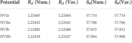
TABLE 1. Deuteron binding energies B_d, in MeV, and nn S-wave phase shift δ₀ at E =5 MeV, in deg, calculated with the Numerov (Num.) or the variational (Var.) methods using the four Norfolk chiral potentials NVIa, NVIIa, NVIb, and NVIIb. Here, we report the results up to the digit from which the two methods start to differ. The experimental value for B_d is $B_d^{\exp }=2.2245$ MeV.

FIGURE 1

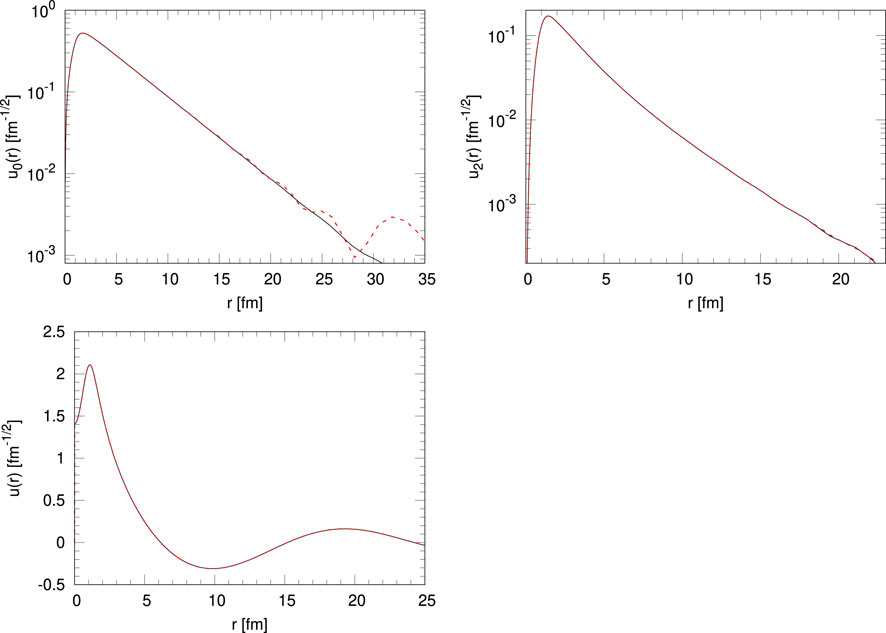
FIGURE 1. Deuteron u₀(r) (left top panel) and u₂(r) (right top panel) functions, and the $nn{}^{1}S_0$ function (left bottom panel) at E =5 MeV are calculated with the variational (dashed red line) and the Numerov (black solid line) methods. The NVIa potential is used. To appreciate the differences between the two methods, the function u₀(r) and u₂(r) are shown in a semilogarithmic scale.

3 Results

We present, in this section, the results for the ${\mathrm{\Gamma }}^D({}^{1}S_0)$ muon capture rate, obtained using the Norfolk potentials and consistent currents, as presented in Section 2.2. In particular, we will use the four Norfolk potentials NVIa, NVIb, NVIIa, and NVIIb, obtained varying the short- and long-range cutoffs (models a or b), and the range of laboratory energies over which the fits have been carried out (models I or II). For each model, the weak vector current and the axial current and the charge operators have been consistently constructed. In particular, we will indicate with the label LO those results obtained including only the LO contributions in the vector current and axial current and charge operators, and with NLO those obtained including, in addition, the NLO contributions to the vector current and axial charge operators. We remind the reader that there are no NLO contributions to the axial current. With the label N2LO we will indicate those results obtained including the N2LO terms of the vector and axial currents, but not the axial charge since they vanish exactly. Finally, with N3LO we will indicate the results obtained when N3LO terms in the vector and axial currents are retained. It should be noted that this is the order in which new LECs appear. The contributions at N3LO for the axial charge are, instead, discarded for the reasons explained in Section 2.2. Finally, we will use the dependence given in Eq. 3 with g_A = 1.2723 and $r_A^2=0.46$ fm² for the axial single-nucleon form factor. However, to establish the uncertainty arising from the rather poor knowledge of $r_A^2$ (see Ref. [34] and the discussion in Section 1 and at the end of Section 2.2), we will also show results obtained with $r_A^2=0.30,0.46,0.62$ fm², so that the 0.16 fm² uncertainty on $r_A^2$ [34] will be taken into account.

First, we begin by proving that the uncertainty arising from the numerical method adopted to study the deuteron and the nn scattering states is well below the 1% level. In fact, Table 2 shows the results obtained with the NVIa potential and currents with up to N3LO contributions, using either the variational or the Numerov method to solve the two-body problem (see Section 2.3). The function $d{\mathrm{\Gamma }}^D({}^{1}S_0)/dp$ (see Eq. 4) calculated with the same potential and currents is shown in Figure 2. As the figure and the table show, the agreement between the results obtained with the two methods is essentially perfect, of the order of 0.01 s⁻¹ in ${\mathrm{\Gamma }}^D({}^{1}S_0)$, well below any other source of error (≃ 0.005%). Therefore, from now on, we will only present results obtained using the variational method, which is numerically less involved than the Numerov one.

TABLE 2

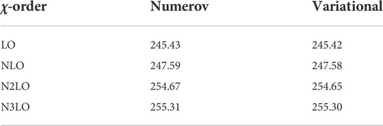
TABLE 2. Total doublet capture rate in the ${}^{1}S_{0}nn$ channel, ${\mathrm{\Gamma }}^D({}^{1}S_0)$ in s⁻¹, calculated using either the Numerov or the variational methods to obtain the deuteron and the nn scattering wave functions. Here, we report the results up to the digit for which the two methods differ. The NVIa potential and consistent currents at the various chiral order are used, and the axial charge radius is taken to be $r_A^2=0.46$ fm².

FIGURE 2

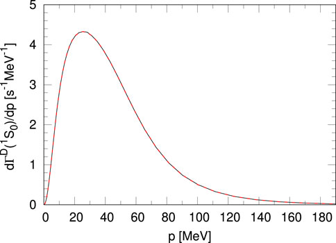
FIGURE 2. Differential doublet capture rate in the ${}^{1}S_{0}nn$ channel, $d{\mathrm{\Gamma }}^D({}^{1}S_0)/dp$ in s⁻¹MeV⁻¹, as a function of the nn relative momentum p in MeV, calculated using either the Numerov (black solid line) or the variational (red dashed line) methods in order to obtain the deuteron and the nn scattering wave functions. The curves are exactly on top of each other. The NVIa potential and consistent currents at N3LO are used. The axial charge radius is taken to be $r_A^2=0.46$ fm².

Table 3 shows the results for ${\mathrm{\Gamma }}^D({}^{1}S_0)$, obtained using all four Norfolk potentials, NVIa, NVIb, NVIIa, and NVIIb, and consistent currents, from LO up to N3LO. The axial charge radius is fixed at $r_A^2=0.46$ fm². As seen in the table, we can provide our best estimate for ${\mathrm{\Gamma }}^D({}^{1}S_0)$, which we calculate simply as the average between the four values at N3LO, ${\mathrm{\Gamma }}^D({}^{1}S_0)=$ 255.8 s⁻¹. Furthermore, we would like to remark that the overall model dependence is quite small, the largest difference being of the order of 1.1 s⁻¹ between the NVIa and NVIIb results, at N3LO. Going into more detail, 1) by comparing the NVIa (NVIIa) and NVIb (NVIIb) results, still at N3LO, we can get a grasp on the cutoff dependence, which turns out to be smaller than 1 s⁻¹ for both models I and II. 2) By comparing the NVIa (NVIb) and NVIIa (NVIIb) results, again at N3LO, we can conclude that the dependence on the NN database used for the LECs’ fitting procedure for the potentials is essentially of the same order. To remain conservative, we decided to define the theoretical uncertainty arising from model dependence as the half range, i.e.,

$\mathrm{\Delta }{\mathrm{\Gamma }}^D\left({}^{1}S_0\right)\left[\text{mod}-\text{dep}\right]\equiv \frac{|{\mathrm{\Gamma }}^D{\left({}^{1}S_0\right)}_{\text{NVIIb}}-{\mathrm{\Gamma }}^D{\left({}^{1}S_0\right)}_{\text{NVIa}}|}{2}.(72)$

TABLE 3

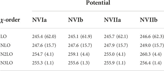
TABLE 3. Total doublet capture rate in the ${}^{1}S_{0}nn$ channel, ${\mathrm{\Gamma }}^D({}^{1}S_0)$ in s⁻¹, calculated using the four Norfolk potentials NVIa, NVIb, NVIIa, and NVIIb, and consistent currents, at the various chiral orders. We also report the uncertainty due to the truncation of the chiral expansion in the current for each order. The axial charge radius is taken to be $r_A^2=0.46$ fm², and the variational method is applied to calculate the deuteron and the nn scattering wave functions.

From this, we obtain $\mathrm{\Delta }{\mathrm{\Gamma }}^D({}^{1}S_0)[\text{mod}-\text{dep}]=0.6$ s⁻¹. We want to remark that this estimate of $\mathrm{\Delta }{\mathrm{\Gamma }}^D({}^{1}S_0)[\text{mod}-\text{dep}]$ does not take into account the error on the fit of the nuclear interaction’s LECs or its chiral truncation. Therefore, it should be considered just as a lower bound of the actual uncertainty.

From Table 3, we can conclude that the chiral-order convergence seems to be quite well under control for all the potential models. In fact, in going from LO to NLO, ${\mathrm{\Gamma }}^D({}^{1}S_0)$ has increased by 2.2 s⁻¹ for the a models, and 2.5 s⁻¹ and 2.4 s⁻¹ for the models NVIb and NVIIb, respectively. This small change is because the only correction appearing at NLO comes from the vector current. Passing from NLO to N2LO, the muon capture rate increases by 7.1 s⁻¹ for the interactions NVIa and NVIIa, and 11.5 s⁻¹ and 11.3 s⁻¹ for the models NVIb and NVIIb, respectively. This can be understood considering that the terms with the Δ-isobar contributions appear at this order for the vector and axial current. The convergence at N3LO shows instead a more involved behavior: for the models NVIa and NVIIa, an ${\mathrm{\Gamma }}^D({}^{1}S_0)$ increase of 0.6 s⁻¹ and 0.9 s⁻¹, respectively, while for the models NVIb and NVIIb, the muon capture rate decreases by 3.5 s⁻¹ and 3.9 s⁻¹, respectively. Even if the results are in reasonable agreement with the expected chiral convergence behavior (in particular for the models a), the chiral convergence of the current shows a significant dependence on the regularization that we tracked back to the axial current corrections and in particular to the different value of the constant c_D (see Section 2.2). We still find remarkable that the results at N3LO obtained with the various potentials, even if their chiral convergence patterns are quite different, turn out to be within 1.1 s⁻¹.

The theoretical uncertainty arising from the chiral-order convergence of the nuclear weak transition operators can be studied using the prescription of Ref. [45]. Here, we report the formula for the error at N2LO only. At this order, for each energy, we define the error for the differential capture rate (to simplify the notation from now on we use ${\mathrm{\Gamma }}^D(p)=d{\mathrm{\Gamma }}^D({}^{1}S_0)/dp$), as

$\mathrm{\Delta }{\mathrm{\Gamma }}^D\left(p\right)\equiv \max \left\{Q^3|{\mathrm{\Gamma }}_{\text{LO}}^D\left(p\right)|,Q^2|{\mathrm{\Gamma }}_{\text{NLO}}^D\left(p\right)-{\mathrm{\Gamma }}_{\text{LO}}^D\left(p\right)|,Q|{\mathrm{\Gamma }}_{\text{N}2\text{LO}}^D\left(p\right)-{\mathrm{\Gamma }}_{\text{NLO}}^D\left(p\right)|\right\},(73)$

where we assumed

$Q=\frac{1}{\mathrm{\Lambda }}\frac{p^8+m_{\pi }^8}{p^7+m_{\pi }^7}(74)$

as in Ref. [46] for the case of the np ↔ dγ reaction. Here, p is the relative momentum of the nn system and we assume a value of Λ ≃ 550 MeV, which is of the order of the cutoff of the adopted interactions. Analogous formulas have been used to study the other orders (see Ref. [45] for details).

In Figure 3, we show the error on $d{\mathrm{\Gamma }}^D({}^{1}S_0)/dp$ order by order in the expansion of the nuclear current up to N3LO for the NVIa interaction. From the figure, the nice convergence of the chiral expansion of the currents is evident. The total error arising from the chiral truncation of the currents on ${\mathrm{\Gamma }}^D({}^{1}S_0)$ is then computed by integrating the error of the differential capture rate over p, namely,

$\mathrm{\Delta }{\mathrm{\Gamma }}^D\left({}^{1}S_0\right)\left[\text{curr}-\text{conv}\right]={\int }_0^{p_{\mathit{max}}}\mathrm{\Delta }{\mathrm{\Gamma }}^D\left(p\right)dp.(75)$

FIGURE 3

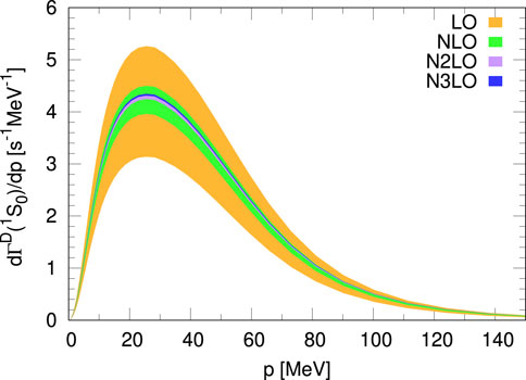
FIGURE 3. Differential doublet capture rate in the ${}^{1}S_{0}nn$ channel, $d{\mathrm{\Gamma }}^D({}^{1}S_0)/dp$ in s⁻¹MeV⁻¹, as a function of the nn relative momentum p in MeV, calculated order by order with the relative errors computed following the prescription of Ref. [45]. The axial charge radius is taken to be $r_A^2=0.46$ fm².

Note that here we assumed the distribution of the truncation error to be uniform, this being a systematic error. Therefore, we do not square it in Eq. 75. Table 3 also shows for each order the error relative to the chiral truncation of the electroweak currents. To be the most conservative as possible, we keep as error the largest obtained with the various interaction models. In the same spirit, we consider the error computed at N2LO, since the calculation at N3LO does not contain all the contributions of the axial charge (see discussion Section 2.2). Therefore, we obtain $\mathrm{\Delta }{\mathrm{\Gamma }}^D({}^{1}S_0)[\text{curr}-\text{conv}]=4.4$ s⁻¹. In comparison, the same calculation at N3LO would give as an error $\mathrm{\Delta }{\mathrm{\Gamma }}^D({}^{1}S_0)[\text{curr}-\text{conv}]{|}_{\text{N}3\text{LO}}=1.4$ s⁻¹. We want to remark that the uncertainty computed here arises only from the chiral truncation of the currents and it represents only a lower bound of the total chiral error.

Finally, Table 4 shows the results obtained with all the interactions and consistent currents up to N3LO for the three values of the axial charge radius, $r_A^2=0.30,0.46,0.62$ fm². This allows us to understand the importance of this last source of theoretical uncertainty. The three values are chosen to span the range of values proposed in Ref. [34], being the lower limit, central value, and upper limit for $r_A^2$. We also verified that ${\mathrm{\Gamma }}^D({}^{1}S_0)$ has a linear dependence on $r_A^2$. As a consequence, performing the calculation for the three mentioned values of $r_A^2$ is essentially equivalent to the “standard” error propagation. Again, we define the theoretical uncertainty $\mathrm{\Delta }{\mathrm{\Gamma }}^D({}^{1}S_0)[r_A^2]$ arising from this last source as the half-range of the results, i.e.,

$\mathrm{\Delta }{\mathrm{\Gamma }}^D\left({}^{1}S_0\right)\left[r_A^2\right]\equiv \underset{\mathit{pot}}{\max }\left\{\frac{|{\mathrm{\Gamma }}^D{\left({}^{1}S_0\right)}_{r_A^2=0.30}-{\mathrm{\Gamma }}^D{\left({}^{1}S_0\right)}_{r_A^2=0.62}|}{2}\right\},(76)$

where max_pot indicates that we take the maximum value among the different interactions considered. From the table, we can conclude that $\mathrm{\Delta }{\mathrm{\Gamma }}^D({}^{1}S_0)[r_A^2]=2.9$ s⁻¹, which is found to be essentially model-independent.

TABLE 4

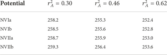
TABLE 4. Total doublet capture rate in the ${}^{1}S_{0}nn$ channel, ${\mathrm{\Gamma }}^D({}^{1}S_0)$ in s⁻¹, is calculated using all the different interactions and consistent currents up to N3LO, and three different values of $r_A^2$, $r_A^2=0.30,0.46,0.62$ fm². The variational method is applied to calculate the deuteron and the nn scattering wave functions.

In conclusion, our final result for ${\mathrm{\Gamma }}^D({}^{1}S_0)$ is

${\mathrm{\Gamma }}^D\left({}^{1}S_0\right)=255.8\left(0.6\right)\left(4.4\right)\left(2.9\right){\mathrm{s}}^{-1},(77)$

where the three uncertainties arise from model dependence, chiral convergence, and the experimental error in the axial charge radius r_A. The overall systematic uncertainty becomes 5.0 s⁻¹ when the various contributions are summed. The uncertainty on $r_A^2$ is instead statistical and, therefore, must be treated separately. This result can be compared with those of Refs. [10, 12]. In Ref. [10], we found a value of 253.5 (1.2) s⁻¹, the error taking care of the cutoff dependence and the uncertainty in the d_R LEC fitting procedure. When only the cutoff dependence is considered, it reduces to 0.2 s⁻¹, somewhat smaller than the present 0.6 s⁻¹. The central values that we obtained and the one quoted in Ref. [10], even if the chiral potentials are very different, are instead in reasonable agreement. In Ref. [12], it was found that ${\mathrm{\Gamma }}^D({}^{1}S_0)=252.8(4.6)(3.9){\mathrm{s}}^{-1}$, where the first error is due to the truncation in the chiral expansion and the second is due to the uncertainty in the nucleon axial radius r_A. These two errors should be compared with our 5.0 s⁻¹ and 2.9 s⁻¹. The agreement for the first error is very nice, while the small difference in the second error is certainly due to the fact that in Ref. [12] a larger uncertainty for $r_A^2$ was used (0.22 fm² vs. the present 0.16 fm²). Also, in this case, the agreement between the central values is good, even if the potential models adopted are very different. This could suggest that the observable ${\mathrm{\Gamma }}^D({}^{1}S_0)$ is not sensitive to the nuclear potential model, as long as this can properly reproduce the deuteron and the nn scattering systems (as, in fact, any realistic modern potential usually does).

4 Conclusion and outlook

We investigated, for the first time, with local nuclear potential models derived in χEFT and consistent currents, the muon capture on deuteron, in the ${}^{1}S_0$ initial nn scattering state. The use of this framework allowed us to 1) provide a new estimate for the capture rate ${\mathrm{\Gamma }}^D({}^{1}S_0)$, which turned out to agree with the results already present in the literature and obtained still in χEFT, but with different (non-local) potential models [10, 12]; 2) accompany this estimate with a determination of the theoretical uncertainty, which arises from model dependence, chiral convergence, and the uncertainty in the single-nucleon axial charge radius r_A. We also verified that the uncertainty arising from the numerical technique adopted to solve the two-body bound- and scattering-state problem is completely negligible.

Our final result is ${\mathrm{\Gamma }}^D({}^{1}S_0)=255.8(0.6)(4.4)(2.9)$ s⁻¹, where the three errors come from the three sources of uncertainty just mentioned. To provide an indicative value for the overall uncertainty, we propose to sum the systematic uncertainties arising from sources 1) and 2), obtaining the value of 5.0 s⁻¹. Then, this error can be summed in quadrature with the one of source 3), 2.9 s⁻¹. Therefore, we obtain ${\mathrm{\Gamma }}^D({}^{1}S_0)=255.8(5.8)$ s⁻¹. We remark again that the value of 5.8 s⁻¹ for the overall uncertainty is only indicative, and the preferable procedure should be to treat the three errors, 0.6 s⁻¹, 4.4 s⁻¹, and 2.9 s⁻¹, separately. Moreover, it is important to remind that the errors coming from the sources 1) and 2) can be considered only as lower limits of the actual uncertainty coming from the model dependence and the chiral truncation.

Given the success of this calculation in determining ${\mathrm{\Gamma }}^D({}^{1}S_0)$ and its uncertainty, with a procedure less involved than the one of Ref. [12], which still leads to similar results, we plan to proceed with applying this framework to the calculation of Γ^D, retaining all the nn partial waves up to J = 2 and L = 3. These are known to provide contributions to Γ^D up to 1 s⁻¹ [9]. In parallel, we plan to study the muon capture processes also on ³He and ⁶Li, in the footsteps of Ref. [27]. Here, the Norfolk potentials were used in conjunction with the variational and Green’s function Monte Carlo techniques to solve for the A = 3, 6 bound states, and the final results were found to disagree, to some level, with the experimental data. It will be interesting to verify these outcomes, using the hyperspherical harmonics method to solve for the A = 3, 6 nuclei [47–49]. Last but not least, we plan to apply this same framework to weak processes of interest for solar standard models and solar neutrino fluxes, i.e., the proton weak capture on proton (reaction 2), and on ³He (the so-called hep reaction). In this second case, it is remarkable that a consistent χEFT calculation is still missing (see Refs. [50–52]). For both reactions, we will be able to provide a value for the astrophysical S-factor at zero energy accompanied by an estimate of the theoretical uncertainty.

Data availability statement

The original contributions presented in the study are included in the article; further inquiries can be directed to the corresponding author.

Author contributions

LC and LM shared the idea, the formula derivation, and the computer code implementation of this work. LM was mainly responsible for the drafting of the manuscript. AG contributed to reviewing the codes and running them in order to obtain the final results presented here, while MP and MV gave valuable suggestions during the setting up of the calculation. All the authors contributed equally to reviewing and correcting the draft of the manuscript.

Funding

AG acknowledges the support provided by the U.S. Department of Energy, Office of Nuclear Science, under Contract No. DE-AC05-06OR23177, while MP acknowledges the support from the U.S. Department of Energy through the FRIB Theory Alliance Award No. DE-SC0013617.

Acknowledgments

The authors also acknowledge the Istituto Nazionale di Fisica Nucleare (INFN), Sezione di Pisa, for providing the computational resources. The final calculation was performed using resources of the National Energy Research Scientific Computing Center (NERSC), a U.S. Department of Energy Office of Science User Facility located at Lawrence Berkeley National Laboratory, operated under Contract No. DE-AC02-05CH11231.

Conflict of interest

The authors declare that the research was conducted in the absence of any commercial or financial relationships that could be construed as a potential conflict of interest.

Publisher’s note

All claims expressed in this article are solely those of the authors and do not necessarily represent those of their affiliated organizations, or those of the publisher, the editors, and the reviewers. Any product that may be evaluated in this article, or claim that may be made by its manufacturer, is not guaranteed or endorsed by the publisher.

References

1. Measday DF. The nuclear physics of muon capture. Phys Rep (2001) 354:243–409. doi:10.1016/s0370-1573(01)00012-6

CrossRef Full Text | Google Scholar

2. Wang IT, Anderson EW, Bleser EJ, Lederman LM, Meyer SL, Rosen JL, et al. Muon capture in (p μ d)+ molecules. Phys Rev (1965) 139:B1528–38. doi:10.1103/physrev.139.b1528

CrossRef Full Text | Google Scholar

3. Bertin A, Vitale A, Placci A, Zavattini E. Muon capture in gaseous deuterium. Phys Rev D (1973) 8:3774–93. doi:10.1103/physrevd.8.3774

CrossRef Full Text | Google Scholar

4. Bardin G, Duclos J, Martino J, Bertin A, Capponi M, Piccinini M, et al. A measurement of the muon capture rate in liquid deuterium by the lifetime technique. Nucl Phys A (1986) 453:591–604. doi:10.1016/0375-9474(86)90253-8

CrossRef Full Text | Google Scholar

5. Cargnelli M, et al. Workshop on fundamental μ physics, los alamos, 1986, LA 10714C. In: M Morita, H Ejiri, H Ohtsubo, and T Sato, editors. Nuclear weak process and nuclear structure, Yamada Conference XXIII. Singapore: World Scientific (1989). p. 115.

Google Scholar

6. Kammel P. Precision muon capture at PSI. PoS (2013) CD12:016.

Google Scholar

7. Marcucci LE. Muon capture on deuteron and ³He: A personal review. Int J Mod Phys A (2012) 27:1230006. doi:10.1142/s0217751x12300062

CrossRef Full Text | Google Scholar

8. Adam J, Tater M, Truhlik E, Epelbaum E, Machleidt R, Ricci P. Calculation of doublet capture rate for muon capture in deuterium within chiral effective field theory. Phys Lett B (2012) 709:93–100. doi:10.1016/j.physletb.2012.01.065

CrossRef Full Text | Google Scholar

9. Marcucci LE, Piarulli M, Viviani M, Girlanda L, Kievsky A, Rosati S, et al. Muon capture on deuteron and ³He. Phys Rev C (2011) 83:014002. doi:10.1103/physrevc.83.014002

CrossRef Full Text | Google Scholar

10. Marcucci LE, Kievsky A, Rosati S, Schiavilla R, Viviani M. Chiral effective field theory predictions for muon capture on deuteron and ³He. Phys Rev Lett (2012) 108:052502. [Erratum: Phys. Rev. Lett. 121, (2018) 049901]. doi:10.1103/physrevlett.108.052502

PubMed Abstract | CrossRef Full Text | Google Scholar

11. Golak J, Skibiński R, Witała H, Topolnicki K, Elmeshneb AE, Kamada H, et al. Break-up channels in muon capture on ³He. Phys Rev C (2014) 90:024001. [Addendum: Phys.Rev.C 90, 029904 10.1103/physrevc.90.029904(2014)].

CrossRef Full Text | Google Scholar

12. Acharya B, Ekström A, Platter L. Effective-field-theory predictions of the muon-deuteron capture rate. Phys Rev C (2018) 98:065506. doi:10.1103/physrevc.98.065506

CrossRef Full Text | Google Scholar

13. Entem DR, Machleidt R. Accurate charge dependent nucleon nucleon potential at fourth order of chiral perturbation theory. Phys Rev C (2003) 68:041001. doi:10.1103/physrevc.68.041001

CrossRef Full Text | Google Scholar

14. Machleidt R, Entem DR. Chiral effective field theory and nuclear forces. Phys Rep (2011) 503:1–75. doi:10.1016/j.physrep.2011.02.001

CrossRef Full Text | Google Scholar

15. Gazit D, Quaglioni S, Navrátil P. Three-nucleon low-energy constants from the consistency of interactions and currents in chiral effective field theory. Phys Rev Lett (2009) 103:102502. [Erratum: Phys. Rev. Lett. 122, (2019) 029901]. doi:10.1103/physrevlett.103.102502

PubMed Abstract | CrossRef Full Text | Google Scholar

16. Carlsson BD, Ekström A, Forssén C, Strömberg DF, Jansen GR, Lilja O, et al. Uncertainty analysis and order-by-order optimization of chiral nuclear interactions. Phys Rev X (2016) 6:011019. doi:10.1103/physrevx.6.011019

CrossRef Full Text | Google Scholar

17. Acharya B, Ekström A, Odell D, Papenbrock T, Platter L. Corrections to nucleon capture cross sections computed in truncated Hilbert spaces. Phys Rev C (2017) 95:031301. doi:10.1103/physrevc.95.031301

CrossRef Full Text | Google Scholar

18. Piarulli M, Tews I. Local nucleon-nucleon and three-nucleon interactions within chiral effective field theory. Front Phys (2020) 7:245. doi:10.3389/fphy.2019.00245

CrossRef Full Text | Google Scholar

19. Piarulli M, Girlanda L, Schiavilla R, Kievsky A, Lovato A, Marcucci LE, et al. Local chiral potentials with Δ-intermediate states and the structure of light nuclei. Phys Rev C (2016) 94:054007. doi:10.1103/physrevc.94.054007

CrossRef Full Text | Google Scholar

20. Baroni A, Schiavilla R, Marcucci LE, Girlanda L, Kievsky A, Lovato A, et al. Local chiral interactions, the tritium Gamow-Teller matrix element, and the three-nucleon contact term. Phys Rev C (2018) 98:044003. doi:10.1103/physrevc.98.044003

CrossRef Full Text | Google Scholar

21. Schiavilla R, Baroni A, Pastore S, Piarulli M, Girlanda L, Kievsky A, et al. Local chiral interactions and magnetic structure of few-nucleon systems. Phys Rev C (2019) 99:034005. doi:10.1103/physrevc.99.034005

CrossRef Full Text | Google Scholar

22. Gnech A, Schiavilla R. Magnetic structure of few-nucleon systems at high momentum transfers in a χEFT approach (2022). arXiv:2207.05528.

Google Scholar

23. Piarulli M, Baroni A, Girlanda L, Kievsky A, Lovato A, Lusk E, et al. Light-nuclei spectra from chiral dynamics. Phys Rev Lett (2018) 120:052503. doi:10.1103/PhysRevLett.120.052503

PubMed Abstract | CrossRef Full Text | Google Scholar

24. Gandolfi S, Lonardoni D, Lovato A, Piarulli M. Atomic nuclei from quantum Monte Carlo calculations with chiral EFT interactions. Front Phys (2020) 8:117. doi:10.3389/fphy.2020.00117

CrossRef Full Text | Google Scholar

25. King GB, Andreoli L, Pastore S, Piarulli M, Schiavilla R, Wiringa RB, et al. Chiral effective field theory calculations of weak transitions in light nuclei. Phys Rev C (2020) 102:025501. doi:10.1103/physrevc.102.025501

CrossRef Full Text | Google Scholar

26. King GB, Andreoli L, Pastore S, Piarulli M. Weak transitions in light nuclei. Front Phys (2020) 8:363. doi:10.3389/fphy.2020.00363

CrossRef Full Text | Google Scholar

27. King GB, Pastore S, Piarulli M, Schiavilla R. Partial muon capture rates in A=3 and A=6 nuclei with chiral effective field theory. Phys Rev C (2022) 105:L042501. doi:10.1103/physrevc.105.l042501

CrossRef Full Text | Google Scholar

28. Cirigliano V, Dekens W, De Vries J, Graesser ML, Mereghetti E, Pastore S, et al. Renormalized approach to neutrinoless double- β decay. Phys Rev C (2019) 100:055504. doi:10.1103/physrevc.100.055504

CrossRef Full Text | Google Scholar

29. King GB, Baroni A, Cirigliano V, Gandolfi S, Hayen L, Mereghetti E, et al. Ab initio calculation of the β decay spectrum of ⁶He (2022). ArXiv:2207.11179.

Google Scholar

30. Piarulli M, Bombaci I, Logoteta D, Lovato A, Wiringa RB. Benchmark calculations of pure neutron matter with realistic nucleon-nucleon interactions. Phys Rev C (2020) 101:045801. doi:10.1103/physrevc.101.045801

CrossRef Full Text | Google Scholar

31. Lovato A, Bombaci I, Logoteta D, Piarulli M, Wiringa RB. Benchmark calculations of infinite neutron matter with realistic two- and three-nucleon potentials. Phys Rev C (2022) 105:055808. doi:10.1103/physrevc.105.055808

CrossRef Full Text | Google Scholar

32. Acharya B, Platter L, Rupak G. Universal behavior of p-wave proton-proton fusion near threshold. Phys Rev C (2019) 100:021001. doi:10.1103/physrevc.100.021001

CrossRef Full Text | Google Scholar

33. Marcucci LE, Schiavilla R, Viviani M. Proton-proton weak capture in chiral effective field theory. Phys Rev Lett (2013) 110:192503. [Erratum: Phys. Rev. Lett. 123, (2019) 019901]. doi:10.1103/physrevlett.110.192503

PubMed Abstract | CrossRef Full Text | Google Scholar

34. Hill RJ, Kammel P, Marciano WJ, Sirlin A. Nucleon axial radius and muonic hydrogen—A new analysis and review. Rep Prog Phys (2018) 81:096301. doi:10.1088/1361-6633/aac190

PubMed Abstract | CrossRef Full Text | Google Scholar

35. Walecka J. Theorethical nuclear and subnuclear Physics. London: Imperial College Press (1995).

Google Scholar

36. Navarro Pérez R, Amaro JE, Ruiz Arriola E. Erratum: Coarse-grained potential analysis of neutron-proton and proton-proton scattering below the pion production threshold [Phys. Rev. C88, 064002 (2013)]. Phys Rev C (2013) 88:064002. [Erratum: Phys. Rev. C 91, (2015) 029901]. doi:10.1103/physrevc.91.029901

CrossRef Full Text | Google Scholar

37. Navarro Pérez R, Amaro JE, Ruiz Arriola E. Coarse grained nn potential with chiral two-pion exchange. Phys Rev C (2014) 89:024004. doi:10.1103/physrevc.89.024004

CrossRef Full Text | Google Scholar

38. Navarro Pérez R, Amaro JE, Ruiz Arriola E. Statistical error analysis for phenomenological nucleon-nucleon potentials. Phys Rev C (2014) 89:064006. doi:10.1103/physrevc.89.064006

CrossRef Full Text | Google Scholar

39. Krebs H, Epelbaum E, Meissner U. Nuclear forces with Δ excitations up to next-to-next-to-leading order, part I: Peripheral nucleon-nucleon waves. Eur Phys J A (2007) 32:127–37. doi:10.1140/epja/i2007-10372-y

CrossRef Full Text | Google Scholar

40. Baroni A, Girlanda L, Pastore S, Schiavilla R, Viviani M. Nuclear axial currents in chiral effective field theory. Phys Rev C (2016) 93:015501. doi:10.1103/physrevc.93.015501

CrossRef Full Text | Google Scholar

41. Meyer AS, Betancourt M, Gran R, Hill RJ. Deuterium target data for precision neutrino-nucleus cross sections. Phys Rev D (2016) 93:113015. doi:10.1103/physrevd.93.113015

CrossRef Full Text | Google Scholar

42. Abramowitz M, Stegun IA. Handbook of mathematical functions with formulas, graphs, and mathematical tables, vol. 55. Washington, DC, USA: US Government printing office (1964).

Google Scholar

43. Kohn W. Variational methods in nuclear collision problems. Phys Rev (1948) 74:1763–72. doi:10.1103/physrev.74.1763

CrossRef Full Text | Google Scholar

44. Johnson BR. The renormalized Numerov method applied to calculating bound states of the coupled-channel Schroedinger equation. J Chem Phys (1978) 69:4678–88. doi:10.1063/1.436421

CrossRef Full Text | Google Scholar

45. Epelbaum E, Krebs H, Meißner UG. Improved chiral nucleon-nucleon potential up to next-to-next-to-next-to-leading order. Eur Phys J A (2015) 51:53. doi:10.1140/epja/i2015-15053-8

CrossRef Full Text | Google Scholar

46. Acharya B, Bacca S. Gaussian process error modeling for chiral effective-field-theory calculations of np ↔ dγ at low energies. Phys Lett B (2022) 827:137011. doi:10.1016/j.physletb.2022.137011

CrossRef Full Text | Google Scholar

47. Marcucci LE, Dohet-Eraly J, Girlanda L, Gnech A, Kievsky A, Viviani M. The hyperspherical harmonics method: A tool for testing and improving nuclear interaction models. Front Phys (2020) 8:69. doi:10.3389/fphy.2020.00069

CrossRef Full Text | Google Scholar

48. Gnech A, Viviani M, Marcucci LE. Calculation of the ⁶Li ground state within the hyperspherical harmonic basis. Phys Rev C (2020) 102:014001. doi:10.1103/physrevc.102.014001

CrossRef Full Text | Google Scholar

49. Gnech A, Marcucci LE, Schiavilla R, Viviani M. Comparative study of ⁶He β-decay based on different similarity-renormalization-group evolved chiral interactions. Phys Rev C (2021) 104:035501. doi:10.1103/physrevc.104.035501

CrossRef Full Text | Google Scholar

50. Marcucci LE, Schiavilla R, Viviani M, Kievsky A, Rosati S, Beacom JF. Weak proton capture on ³He. Phys Rev C (2001) 63:015801. doi:10.1103/physrevc.63.015801

CrossRef Full Text | Google Scholar

51. Park TS, Marcucci LE, Schiavilla R, Viviani M, Kievsky A, Rosati S, et al. Parameter free effective field theory calculation for the solar proton fusion and hep processes. Phys Rev C (2003) 67:055206. doi:10.1103/physrevc.67.055206

CrossRef Full Text | Google Scholar

52. Adelberger EG, Garcia A, Robertson RGH, Snover KA, Balantekin AB, Heeger K, et al. Solar fusion cross sections. II. Theppchain and CNO cycles. Rev Mod Phys (2011) 83:195–245. doi:10.1103/revmodphys.83.195

CrossRef Full Text | Google Scholar