Demixing population activity in higher cortical areas

Introduction

Higher-order cortical areas such as the prefrontal cortex receive and integrate information from many other areas of the brain. The activity of neurons in these areas often reflects this mix of influences. Typical neural responses are shaped both by the internal dynamics of these systems as well as by various external events such as the perception of a stimulus or a reward (Rao et al., 1997; Romo et al., 1999; Brody et al., 2003; Averbeck et al., 2006; Feierstein et al., 2006; Gold and Shadlen, 2007; Seo et al., 2009). As a result, neural responses are extremely complex and heterogeneous, even in animals that are performing relatively facile tasks such as simple stimulus–response associations (Gold and Shadlen, 2007).

To make sense of these data, researchers typically seek to relate the firing rate of a neuron to one of various experimentally controlled task parameters, such as a sensory stimulus, a reward, or a decision that an animal takes. To this end, a number of statistical tools are exploited such as regression (Romo et al., 2002; Brody et al., 2003; Sugrue et al., 2004; Kiani and Shadlen, 2009; Seo et al., 2009), signal detection theory (Feierstein et al., 2006; Kepecs et al., 2008), or discriminant analysis (Rao et al., 1997). The population response is then characterized by quantifying how each neuron in the population responds to a particular task parameter. Subsequently, neurons can be attributed to different (possibly overlapping) response categories, and population responses can be constructed by averaging the time-varying firing rates within such a category.

This classical, single-cell based approach to electrophysiological population data has been quite successful in clarifying what information neurons in higher-order cortical areas represent. However, the approach rarely succeeds in giving a complete account of the recorded activity on the population level. For instance, many interesting features of the population response may go unnoticed if they have not been explicitly looked for. Furthermore, the strongly distributional nature of the population response, in which individual neurons can be responsive to several task parameters at once, is often left in the shadows.

Principal component analysis (PCA) and other dimensionality reduction techniques seek to alleviate these problems by providing methods that summarize neural activity at the population level (Nicolelis et al., 1995; Friedrich and Laurent, 2001; Zacksenhouse and Nemets, 2008; Yu et al., 2009; Machens et al., 2010). However, such “unsupervised” techniques will usually neglect information about the relevant task variables. While the methods do provide a succinct and complete description of the population response, the description may yield only limited insights into how different task parameters are represented in the population of neurons.

In this paper, we propose an exploratory data analysis method that seeks to maintain the major benefits of PCA while also extracting the relevant task variables from the data. The primary goal of our method is to improve on dimensionality reduction techniques by explicitly taking knowledge about task parameters into account. The method has previously been applied to data from the prefrontal cortex to separate stimulus- from time-related activities (Machens et al., 2010). Here, we describe the method in greater detail, derive it from first principles, investigate its performance under noise, and generalize it to more than two task parameters. Our hope is that this method provides a better visualization of a given data set, thereby yielding new insights into the function of higher-order areas. We will first explain the main ideas in the context of a simple example, then show how these ideas can be generalized, and finally discuss some caveats and limitations of our approach.

Results

Response Heterogeneity Through Linear Mixing

Recordings from higher-order areas in awake behaving animals often yield a large variety of neural responses (see e.g., Miller, 1999; Churchland and Shenoy, 2007; Jun et al., 2010; Machens et al., 2010). These observations at the level of individual cells could imply a complicated and intricate response at the population level for which a simplified description does not exist. Alternatively, the large heterogeneity of responses may be the result of a simple mixing procedure. For instance, response variety can come about if the responses of individual neurons are random, linear mixtures of a few generic response components (see e.g., Eliasmith and Anderson, 2003).

To illustrate this insight, we will construct a simple toy model. Imagine an animal which performs a two-alternative-forced choice task (Newsome et al., 1989; Uchida and Mainen, 2003). In each trial of such a task, the animal receives a sensory stimulus, s, and then makes a binary decision, d, based on whether s falls into one of two response categories. If the animal decides correctly, it receives a reward. We will assume that the activity of the neurons in our toy model depends only on the stimulus s and the decision d.

To obtain response heterogeneity, we construct the response of each neuron as a random, linear mixture of two underlying response components, one that represents the stimulus, z₁(t,s), and one that represents the decision, z₂(t,d), see Figure 1A. The time-varying firing rate of neuron i is then given by

FIGURE 1

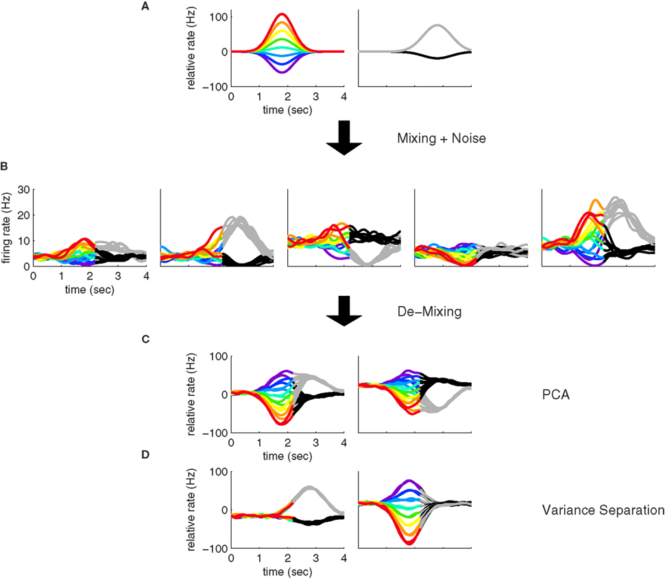
Figure 1. Mixing and demixing of neural responses in a simulated two-alternative forced choice task. (A) We assume that neural responses are linear mixtures of two underlying components, one of which encodes the stimulus (left, colors representing different stimuli), and one of which encodes the binary decision (right) of a two-alternative-forced choice task. For concreteness, we assume that the task comprised M_s = 8 stimuli and M_d = 2 decisions. (B) Single cell responses are random combinations of these two components. We assume that N = 50 neurons have been recorded, five of which are shown here. The noisy variability of the responses was obtained by transforming the deterministic, linear mixture of each neuron into 10 inhomogeneous Poisson spike trains, and then re-estimating the firing rates by low-pass filtering and averaging the spike trains. This type of noise may be considered more realistic, even if it deviates from the assumptions in the main text. In our numerical example, this did not prove to be a problem. To systematically address such problems, however, one may apply a variance-stabilizing transformation to the data, such as taking the square-root of the firing rates before computing the covariance matrix (see e.g., Efron, 1982). (C) PCA uncovers the underlying two-dimensionality of the data, but the resulting coordinates do not demix the separate sources of firing rate variance. (D) By explicitly contrasting these separate sources, we can retrieve the original components up to a sign.

Here, the parameters a_i1 and a_i2 are the mixing coefficients of the neuron, the bias parameter c_i describes a constant offset, and the term η_i(t) denotes additive, white noise. We assume that the noise of different neurons can be correlated so that

where the angular brackets denote averaging over time, and H_ij is the noise covariance between neuron i and j. We will assume that there are N neurons and, for notational compactness, we will assemble their activities into one large vector, r(t,s,d) = (r₁(t,s,d),…,r_N(t,s,d))^T. After doing the same for the mixing coefficients, the constant offset, and the noise, we can write equivalently,

Without loss of generality, we can furthermore assume that the mixing coefficients are normalized so that for i ∈{1,2}. Since we assume that the mixing coefficients are drawn at random, and independently of each other, the first and second coefficient will be uncorrelated, so that on average, , implying that a₁ and a₂ are approximately orthogonal.

With this formulation, individual neural responses mix information about the stimulus s and the decision d, leading to a variety of responses, as shown in Figure 1B. While with only two underlying components, the overall heterogeneity of responses remains limited, the response heterogeneity increases strongly when more components are allowed (see Figures 3A,B for an example with three components).

Principal Component Analysis Fails to Demix the Responses

The standard approach to deal with such data sets is to sort cells into categories. In our example, this approach may yield two overlapping categories of cells, one for cells that respond to the stimulus and one for cells that respond to the decision. While this approach tracks down which variables are represented in the population, it will fail to quantify the exact nature of the population activity, such as the precise co-evolution of the neural population activity over time.

A common approach to address these types of problems are dimensionality reduction methods such as PCA (Nicolelis et al., 1995; Friedrich and Laurent, 2001; Hastie et al., 2001; Zacksenhouse and Nemets, 2008; Machens et al., 2010). The main aim of PCA is to find a new coordinate system in which the data can be represented in a more succinct and compact fashion. In our toy example, even though we may have many neurons with different responses (N = 50 in Figure 1, with five examples shown in Figure 1B), the activity of each neuron can be represented by a linear combination of only two components. In the N-dimensional space of neural activities, the two components, z₁(t,s) and z₂(t,d), can be viewed as two coordinates of a coordinate system whose axes are given by the vectors of mixing coefficients, a₁ and a₂. Since the first two coordinates capture all the relevant information, the components live in a two-dimensional subspace. Using PCA, we can retrieve the two-dimensional subspace from the data. While the method allows us to reduce the dimensionality and complexity of the data dramatically, PCA will in general only retrieve the two-dimensional subspace, but not the original coordinates, z₁(t,s) and z₂(t,d).

To see this, we will briefly review PCA and show what it does to the data from our toy model. PCA commences by computing the covariances of the firing rates between all pairwise combination of neurons. Let us define the mean firing rate of neuron i as the average number of spikes that this neuron emits, so that

We will use the angular brackets in the second line as a short-hand for averaging. The variables to be averaged over are indicated as subscript on the right bracket. Here, the average runs over all time points t, all stimuli s, and all decisions d. For the vector of mean firing rates we write r = (r₁,…,r_N)^T.

The covariance matrix of the data summarizes the second-order statistics of the data set,

and has size N × N where N is the number of neurons in the data set. Given the covariance matrix, we can compute the firing rate variance that falls along arbitrary directions in state space. For instance, the variance captured by a coordinate axis given by a normalized vector u is simply L = u^TCu. We can then look for the axis that captures most of the variance of the data by maximizing the function L with respect to u subject to the normalization constraint u^Tu = 1. The solution corresponds to the first axis of the coordinate system that PCA constructs. If we are looking for several mutually orthogonal axes, these can be conveniently summarized into an N × n orthogonal matrix, U = [u₁,…,u_n]. To find the maximum amount of variance that falls into the subspace spanned by these axes, we need to maximize

where the trace-operation, tr(·), sums over all the diagonal entries of a matrix, and I_n denotes the n × n identity matrix.

Mathematically, the principal axes u_i correspond to the eigenvectors of the covariance matrix, C, which can nowadays be computed quite easily using numerical methods. Subsequently, the data can be plotted in the new coordinate system. The new coordinates of the data are given by

These new coordinates are called the principal components. Note that the new coordinate system has a different origin from the old one, since we subtracted the vector of mean firing rates, r. Consequently, the principal components can take both negative and positive values. Note also that the principal components are only defined up to a minus sign since every coordinate axis can be reflected along the origin. For our artificial data set, only two eigenvalues are non-zero, so that two principal components suffice to capture the complete variance of the data. The data in these two new coordinates, y₁(t,s,d) and y₂(t,s,d), are shown in Figure 1C.

Our toy model shows how PCA can succeed in summarizing the population response, yet it also illustrates the key problem of PCA: just as the individual neurons, the components mix information about the different task parameters (Figure 1C), even though the original components do not (Figure 1A). The underlying problem is that PCA ignores the causes of firing rate variability. Whether firing rates have changed due to the external stimulus s, due to the internally generated decision d, or due to some other cause, they will enter equally into the computation of the covariance matrix and therefore not influence the choice of the coordinate system constructed by PCA.

To make these notions more precise, we compute the covariance matrix of the simulated data. Inserting Eq. 3 into Eq. 6, we obtain

where M₁₁ and M₂₂ denote firing rate variance due to the first and second component, respectively, M₁₂ denotes firing rate variance due to a mix of the two components, and H is the covariance matrix of the noise. Using the short-hand notations z₁(t) = 〈z₁(t,s)〉_s, z₂(t) = 〈z₂(t,d)〉_d, and z_i = 〈z_i(t)〉_t for i ∈[1,2], the different variances are given by

Principal component analysis will only be able to segregate the stimulus- and decision-dependent variance if the mixture term M₁₂ vanishes and if the variances of the individual components, M₁₁ and M₂₂, are sufficiently different from each other. However, if the two underlying components z₁(t,s) and z₂(t,d) are temporally correlated, then the mixture term M₁₂ will be non-zero. Its presence will then force the eigenvectors of C away from a₁ and a₂. Moreover, even if the mixture term vanishes, PCA may still not be able to retrieve the original mixture coefficients, if the variances of the individual components, M₁₁ and M₂₂ are too close to each other when compared to the magnitude of the noise: in this case the eigenvalue problem becomes degenerate. In general, the covariance matrix therefore mixes different origins of firing rate variance rather than separating them. While PCA allows us to reduce the dimensionality of the data, the coordinate system found may therefore provide only limited insight into how the different task parameters are represented in the neural activities.

Demixing Responses Using Covariances Over Marginalized Data

To solve these problems, we need to separate the different causes of firing rate variability. In the context of our example, we can attribute changes in the firing rates to two separate sources, both of which contribute to the covariance in Eq. 6. First, firing rates may change due to the externally applied stimulus s. Second, firing rates may change due to the internally generated decision d.

To account for these separate sources of variance in the population response, we suggest to estimate one covariance matrix for every source of interest. Such a covariance matrix needs to be specifically targeted toward extracting the relevant source of firing rate variance without contamination by other sources. Naturally, this step is somewhat problem-specific. For our example, we will first focus on the problem of estimating firing rate variance caused by the stimulus separately from firing rate variance caused by the decision. When averaging over all stimuli, we obtain the marginalized firing rates r(t,d) = 〈r(t,s,d)〉_s. The covariance caused by the stimulus is then given by the N × N matrix

We will refer to C_s as the marginalized covariance matrix for the stimulus. We can repeat the procedure for the decision-part of the task. Marginalizing over decisions, we obtain r(t,s) = 〈r(t,s,d)〉_d and

Having two different covariance matrices, one may now perform two separate PCAs, one for each covariance matrix. In turn, one obtains two separate coordinate systems, one in which the principal axes point into the directions of state space along which firing rates vary if the stimulus is changed, the other in which they point into the directions along which firing rates vary if the decision changes.

For the toy model, it is readily seen that the marginalized covariance matrices are given by and with M_s,11 = 〈(z₁(t,s) − z₁(t))²〉 and M_d,22 = 〈(z₂(t,d) − z₂(t))²〉. Consequently, the principal eigenvectors of C_s and C_d will be equivalent to the mixing coefficients a₁ and a₂, at least as long as the variances M_s,11 and M_d,22 are much larger than the size of the noise, which is given by tr(H).

If the noise term is not negligible, it will force the eigenvectors away from the actual mixing coefficients. This problem can be alleviated by using the orthogonality condition, , which implies that there are separate sources of variance for the stimulus- and decision-components. To this end, we can seek to divide the full space into two subspaces, one that captures as much as possible about the stimulus-dependent covariance C_s, and another, that captures as much as possible about the decision-dependent covariance C_d. Our goal will then be to maximize the function

with respect to the two orthogonal matrices U₁ and U₂ whose columns contain the basis vectors of the respective subspaces. The first term in Eq. 15 captures the total variance falling into the subspace spanned by the columns of U₁, and the second term the total variance falling into the subspace given by U₂. Writing U = [U₁,U₂], we obtain an orthogonal matrix for the full space, and the orthogonality conditions are neatly summarized by UU^T = I. As shown in the Appendix, the maximization of Eq. 15 under these orthogonality constraints can be solved by computing the eigenvectors and eigenvalues of the difference of covariance matrices,

In this case, the eigenvectors belonging to the positive eigenvalues of D form the columns of U₁ and the eigenvectors belonging to the negative eigenvalues of D form the columns of U₂. As with PCA, the positive or negative eigenvalues can be sorted according to the amount of variance they capture about C_s and C_d.

For the simulated example, we obtain

where the noise term H has now dropped out. Diagonalization of D results in two clearly separated eigenvalues, M_s,11 and −M_d,11, and in two eigenvectors, a₁ and a₂, that correspond to the original mixing coefficients.

Linking the Population Level and the Single Cell Level

As a result of the above method, we obtain a new coordinate system, whose basis vectors are given by the columns of the matrix U. This coordinate system provides simply a different, and hopefully useful, way of representing the population response. One major advantage of orthogonality is that one can easily move back and forth between the single cell and population level description of the neural activities. Just as in PCA, we can project the original firing rates of the neurons onto the new coordinates,

and the two leading coordinates for the toy model are shown in Figure 1D. These components correspond approximately to the original components, z₁(t,s) and z₂(t,d). In turn, we can reconstruct the activity of each neuron by inverting the coordinate transform,

For every neuron this yields a set of N reconstruction coefficients which correspond to the rows of U.

Since two coordinates were sufficient to capture most of the variance in the toy example, the firing rate of every neuron can be reconstructed by a linear combination of these two components, y₁(t,s,d) and y₂(t,s,d). For each neuron, we thereby obtain two reconstruction coefficients, u_i1 and u_i2. The set of all reconstruction coefficients constitutes a cloud of points in a two-dimensional space. The distribution of this cloud, together with the activities of several example neurons are shown in Figure 2. This plot allows us to link the single cell with the population level by visualizing how the activity of each neuron is composed out of the two underlying components.

FIGURE 2

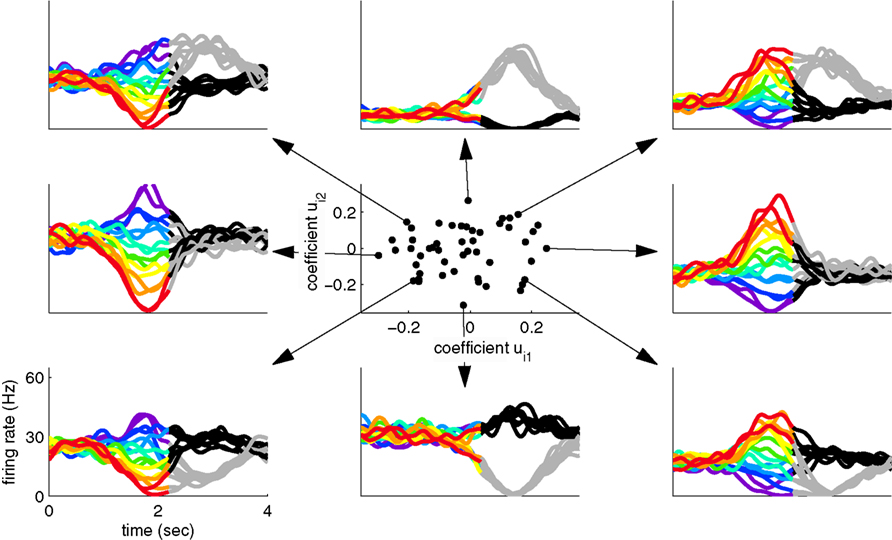
Figure 2. Linking the single cell and population level. Using the coordinate system retrieved by separating variances, we can illuminate the contributions of each component to the individual neural responses. The center shows the contribution of the stimulus- and decision-related components to each individual neuron. The surrounding plots show the activity of eight example neurons, corresponding to the respective dots in the center.

Generalizations to More than Two Parameters

In our toy example, we have assumed that each task parameter is represented by a single component. We note that this is a feature of our specific example. In more realistic scenarios, a single task parameter could potentially be represented by more than one component. For instance, if one set of neurons fires transiently with respect to a stimulus s, but another set of neurons fires tonically, then the firing rate dynamics of the stimulus representation are already two-dimensional, even without taking the decision into account. In such a case, we can still use the method described above to retrieve the two subspaces in which the respective components lie.

However, the number of task parameters will often be larger than two. In the two-alternative-forced choice task, there are at least four parameters that could lead to changes in firing rates: the timing of the task, t, potentially related to anticipation or rhythmic aspects of a task, the stimulus, s, the decision, d, and the reward, r. Even more task parameters could be of interest, such as those extracted from previous trials etc.

These observations raise the question of how the method can be generalized if there are more than two task parameters to account for. To do so, we write the relevant parameters into one long vector θ = (θ₁,θ₂,…,θ_M), and assume that the firing rates of the neurons are linear mixtures of the form

where each task parameter is now represented by more than one component. For each parameter, θ_i, we can compute the marginalized covariance matrix,

which measures the covariance in the firing rates due to changes in the parameter θ_i. Diagonalizing each of these covariance matrices will retrieve the various subspaces corresponding to the different mixture coefficients. For instance, when diagonalizing C₁, we obtain the subspace for the components that depend on the parameter θ₁. The relevant eigenvectors of C₁ will therefore span the same subspace as the mixture coefficients a₁₁, a₁₂, etc., in Eq. 22.

As before, the method’s performance under additive noise can be enhanced by maximizing a single function (see Appendix)

subject to the orthogonality constraint U^TU = I for U = [U₁,U₂,…,U_M]. Maximization of this function will force the firing rate variance due to different parameters θ_i into orthogonal subspaces (as required by the model). If M = 1, then maximization results in a standard PCA. In the case M = 2, maximization requires the diagonalization of the difference of covariance matrices C₁ − C₂, as in Eq. 16. In the case M > 2, various algorithms can be constructed to find local maxima of L (see e.g., Bolla et al., 1998). To our knowledge, a full understanding of the global solution structure of the maximization problem does not exist for M > 2. In the Appendix, we show how to maximize Eq. 24 with standard gradient ascent methods. In any case, it may often be a good idea to use PCA on the full covariance matrix of the data, Eq. 6, to reduce the dimensionality of the data set prior to the demixing procedure. Indeed, this preprocessing step was applied in Machens et al. (2010).

Further Generalizations and Limitations of the Method

The above formulation of the problem may be further generalized by allowing individual components to mix parameters in non-trivial ways. To study this scenario in a simple example, imagine that in the above two-alternative-forced choice task, in addition to the stimulus- and decision-dependent component, there were a purely time-dependent component, z₃(t), locked to the time structure of the task, so that

This scenario is illustrated in Figures 3A,B. As before, we can compute marginalized covariance matrices, that capture the covariance due to the stimuli s, the decisions d, or the time points t. While the marginalized covariance matrices for the stimuli and decisions, C_s and C_d, have one significant eigenvalue each, and thereby capture the relevant component (Figure 3C), the marginalized covariance matrix for time, C_t, now has three significant eigenvalues, and therefore does not allow us to retrieve the purely time-dependent component z₃(t). The reason for this failure is that all three components in Eq. 25 have a time-dependence that cannot be averaged out. By design, the stimulus-averaged first component, z₁(t) = 〈z₁(t,s)〉_s, and the decision-averaged second component, z₂(t) = 〈z₂(t,d)〉_d do not vanish. In other words, the stimulus- and decision-components have intrinsic time-dependent variance that cannot be separated from the stimulus- or decision-induced variance.

FIGURE 3

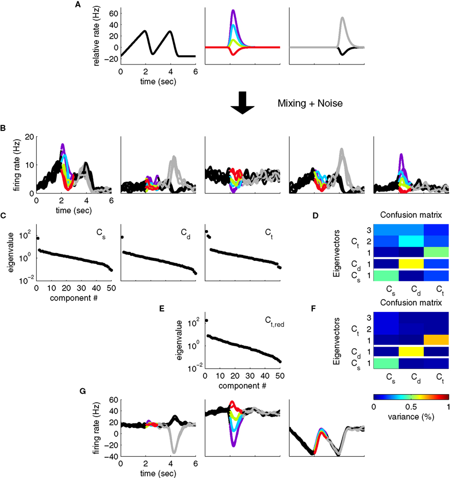
Figure 3. Heterogeneous responses as a result of linear mixture of three components. (A) We now assume that neural responses are constructed from three underlying components, one of which encodes only the task rhythm (left), while the two others encode stimuli and responses, as in Figure 1. (B) Single cell responses are random combinations of these three components. We again assume that N = 50 neurons have been recorded, five of which are shown here, and response noise was generated as in Figure 1. (C) Whereas the marginalized covariance matrices for stimulus and decision, C_s and C_d, have only one significant eigenvalue, the one for time, C_t, features three eigenvalues above the noise floor. (D) The confusion matrix displays the percentage of variance captured by the different components (y-axis) with respect to the different marginalized covariance matrices (x-axis). The C_s row shows, for instance, that the first eigenvector of C_s captures a significant amount of variance from the C_s matrix (which is good), but it also captures a significant amount of variance from the C_t matrix (which is bad). (E) By estimating the time-dependent covariance over a time window limited to t ∈[0,2], we can reduce the number of significant eigenvalues to one. (F) In turn, every row of the confusion matrix has only one entry, showing that every component captures the variance of one marginalized covariance matrix only. (G) The firing rates projected onto the components from (F).

Consequently, the subspace spanned by the first three eigenvectors of C_t overlaps with the respective subspaces spanned by the first eigenvectors of C_s and C_d. One way to visualize this overlap is to take the five relevant eigenvectors (three for C_t, one for C_s, and one for C_d) and compute how much of the variance of each marginalized covariance matrix they capture. To do so, we compute the “confusion matrix”

This confusion matrix measures what percentage of the variance attributed to the j-th cause is captured by the i-th coordinate. For the above example, it is illustrated in Figure 3D. If in one row of this matrix, more than one entry is significantly above 0, then more than one covariance matrix has significant variance along that direction of state space. Whereas the eigenvectors of the C_s and C_d matrix do not interfere with each other, i.e., they are approximately orthogonal, the eigenvectors of the C_t matrix interfere with both the C_s and C_d eigenvectors, i.e., the respective subspaces overlap. The method introduced above will still yield a result in this case, however, the new coordinate system will generally not retrieve the original components.

An ad hoc solution to this problem may be to section the three-dimensional eigenvector subspace of C_t, and identify a direction that is orthogonal to the first eigenvectors of C_s and C_d, which will then correspond to the purely time-dependent component z₃(t). Alternatively, we could restrict the estimation of C_t to the time before stimulus onset, so that the covariance matrix is no longer contaminated by time-dependent variance from the stimulus- or decision-components. The rank of C_t then reduces to one, and the different components separate nicely (Figures 3E,F,G). While feasible in our toy scenario, these ad hoc procedures are not guaranteed to work for real data, when more dimensions are involved, and more complex confusion matrices may result. However, the latter solution demonstrates that by a judicious choice of marginalized covariance matrices, one may sometimes be able to avoid such problems of non-separability.

Connection to Blind Source Separation Methods

In all of these scenarios, we assumed that the firing rates r are linear mixtures of a set of underlying sources z, each with mean 0, so that

The problem that we have been describing then consists in estimating the unknown sources, z, the unknown mixture coefficients, A, and the unknown bias parameters c from the observed data, r. Without loss of generality, we can assume that the sources are centered so that 〈z〉 = 0. Ours is therefore a specific version of the much-studied blind source separation problem (see e.g., Molgedey and Schuster, 1994; Bell and Sejnowski, 1995). In many standard formulations of this problem, one assumes that the sources are uncorrelated, or even statistically independent, which implies that the covariance matrix of the sources, M = 〈zz^T〉_t, is diagonal.

In our case, we do not want to make this assumption, which rules out the use of many blind source separation methods, such as independent component analysis (Hyvärinen et al., 2001). On the upside, we do have additional information, in the form of n task parameters, that provide indirect clues toward the underlying sources. More specifically, we assume that the sources are of the form z_k(t,θ_k) where θ_k denotes a single task parameter, or a specific combination of task parameters. For each task parameter, we can estimate the marginalized covariance matrix C_i, which in turn is given by C_i = AM_iA^T with

As long as different task parameters are distributed over different components, the matrix M_i will be block-diagonal. In the most general case, however, as discussed above, this will not be true. If one parameter is shared among several components, then the respective marginalized covariance matrix will capture variance from all of these components, and maximization of Eq. 24 will not necessarily retrieve the original components. Future work may show how this general, semi-blind source separation problem can be solved by using knowledge about the structure of the marginalized M-matrices. For now, we suggest that in many practical scenarios, a judicious choice of covariance measurements, for instance, by focusing on particular time intervals of a task etc., may help to partly reduce the problem to those that are completely separable, as in Eq. 22.

Discussion

In this article, we addressed the problem of analyzing neural recordings with strong response heterogeneity. A key problem for these data sets is first and foremost the difficulty of visualizing the neural activities at the population level. Simply parsing through individual neural responses is often not sufficient, hence the quest for methods that provide a useful and interpretable summary of the population response.

To provide such a summary, we made one crucial assumption. We assumed that the heterogeneity of neural responses is caused by a simple mixing procedure in which the firing rates of individual neurons are random, linear combinations of a few fundamental components. We believe that such a scenario is likely to be responsible for at least part of the observed response diversity. Higher-level areas of the brain are known to integrate and process information from many other areas in the brain. The presumed fundamental components could be given by the inputs and outputs of these areas. If such components are mixed at random at the level of single cells, then upstream or downstream areas can access the relevant information with simple linear and orthogonal read-outs. Such linear population read-outs have long been known to work quite well in various neural systems (Seung and Sompolinsky, 1993; Salinas and Abbott, 1994).

To retrieve the components from recorded neural activity, and thereby at least partly reduce the response heterogeneity, we suggest to estimate the covariances in the firing rates that can be attributed to the experimentally controlled, external task parameters. Using these marginalized covariance matrices, we showed how to construct an orthogonal coordinate system such that individual coordinates capture the main aspects of the task-related neural activities and the coordinate system as a whole captures all aspects of the neural activities. In the new coordinate system, firing rate variance due to different task parameters is projected onto orthogonal coordinates, making visualization and interpretation of the data particularly easy. We note, though, that the existence of a useful, orthogonal coordinate system is not guaranteed by the method, but can only be a feature of the data. Our method will generally not return useful results if mixing is linear, but not orthogonal, or if mixing is non-linear. Nonetheless, the case of non-orthogonal, linear mixing, may still be investigated through separate PCAs on the different marginalized covariance matrices.

Other methods exist that address similar goals. Most prominently, application of canonical correlation analysis (CCA) to the type of data discussed here would also construct a coordinate system whose choice is influenced by knowledge about the task structure. In our context, CCA would seek a coordinate axis in the state space of neural responses and a coordinate axis in the space of task parameters, such that the correlation between the two is maximized. Whether this method would yield a useful, i.e., interpretable, coordinate system for real data sets remains open to investigation. CCA has recently been proposed as a method to construct population responses in sensory systems (Macke et al., 2008) and as a way to correlate electrophysiological with fMRI data (Biessmann et al., 2009).

Further extensions and generalizations of PCA exist, some of which are specifically targeted to the type of data we have discussed here. The work of Yu et al. (2009), for instance, explicitly addresses the problems that are incurred by estimating firing rates prior to the dimensionality reduction. They show how to combine these two separate steps into a single one using the theory of Gaussian processes. Their work is therefore complementary to ours, and could potentially be incorporated into the methodology introduced here.

Methods to summarize population activity have been employed in many different neurophysiological settings (Friedrich and Laurent, 2001; Stopfer et al., 2003; Paz et al., 2005; Narayanan and Laubach, 2009; Yu et al., 2009). Our main aim here was to modify these methods such that experimentally controlled parameters are taken into account and influence the construction of a new coordinate system. A first application of this method to neural responses from the prefrontal cortex revealed new aspects of a previously studied data set (Machens et al., 2010). Many other data sets with strong response heterogeneity may be amenable to a similar analysis.

Conflict of Interest Statement

The author declares that the research was conducted in the absence of any commercial or financial relationships that could be construed as a potential conflict of interest.

Acknowledgments

I thank Claudia Feierstein, Naoshige Uchida, and Ranulfo Romo for access to their multi-electrode data which have been the main source of inspiration for the present work. I furthermore thank Carlos Brody, Matthias Bethge, Claudia Feierstein, and Thomas Schatz for helpful discussions along various stages of the project. My work is supported by an Emmy-Noether grant from the Deutsche Forschungsgemeinschaft and a Chair d’excellence grant from the Agence Nationale de la Recherche.

References

Averbeck, B. B., Sohn, J.-W., and Lee, D. (2006). Activity in prefrontal cortex during dynamic selection of action sequences. Nat. Neurosci. 9, 276–282.

Pubmed Abstract | Pubmed Full Text | CrossRef Full Text

Bell, A. J., and Sejnowski, T. J. (1995). An information-maximization approach to blind separation and blind deconvolution. Neural Comput. 7, 1129–1159.

Pubmed Abstract | Pubmed Full Text | CrossRef Full Text

Biessmann, F., Meinecke, F. C., Gretton, A., Rauch, A., Rainer, G., Logothetis, N., and Müller, K. R. (2009). Temporal kernel canonical correlation analysis and its application in multimodal neuronal data analysis. Mach. Learn. 79, 5–27.

CrossRef Full Text

Bolla, M., Michaletzky, G., Tusnády, G., and Ziermann, M. (1998). Extrema of sums of heterogeneous quadratic forms. Linear Algebra Appl. 269, 331–365.

CrossRef Full Text

Brody, C. D., Hernandez, A., Zainos, A., and Romo, R. (2003). Timing and neural encoding of somatosensory parametric working memory in macaque prefrontal cortex. Cereb. Cortex 13, 1196–1207.

Pubmed Abstract | Pubmed Full Text | CrossRef Full Text

Churchland, M. M., and Shenoy, K. V. (2007). Temporal complexity and heterogeneity of single-neuron activity in premotor and motor cortex. J. Neurophysiol. 97, 4235–4257.

Pubmed Abstract | Pubmed Full Text | CrossRef Full Text

Efron, B. (1982). Transformation theory: how normal is a family of distributions? Ann. Stat. 10, 328–339.

Eliasmith, C., and Anderson, C. H. (2003). Neural Engineering: Computation, Representation, and Dynamics in Neurobiological Systems. Cambridge, MA: MIT Press.

Feierstein, C. E., Quirk, M. C., Uchida, N., Sosulski, D. L., and Mainen, Z. F. (2006). Representation of spatial goals in rat orbitofrontal cortex. Neuron 51, 495–507.

Pubmed Abstract | Pubmed Full Text | CrossRef Full Text

Friedrich, R. W., and Laurent, G. (2001). Dynamic optimization of odor representations by slow temporal patterning of mitral cell activity. Science 291, 889–894.

Pubmed Abstract | Pubmed Full Text | CrossRef Full Text

Gold, J. I., and Shadlen, M. N. (2007). The neural basis of decision making. Annu. Rev. Neurosci. 30, 535–574.

Pubmed Abstract | Pubmed Full Text | CrossRef Full Text

Hastie, T., Tibshirani, R., and Friedman, J. (2001). The Elements of Statistical Learning Theory. New York: Springer.

Hyvärinen, A., Karhunen, J., and Oja, E. (2001). Independent Component Analysis. New York: Wiley InterScience.

Jun, J. K., Miller, P., Hernández, A., Zainos, A., Lemus, L., Brody, C., and Romo, R. (2010). Heterogeneous population coding of a short-term memory and decision-task. J. Neurosci. 30, 916–929.

Pubmed Abstract | Pubmed Full Text | CrossRef Full Text

Kepecs, A., Uchida, N., Zariwala, H. A., and Mainen, Z. F. (2008). Neural correlates, computation and behavioural impact of decision confidence. Nature 455, 227–231.

Pubmed Abstract | Pubmed Full Text | CrossRef Full Text

Kiani, R., and Shadlen, M. N. (2009). Representation of confidence associated with a decision by neurons in the parietal cortex. Science 324, 759–764.

Pubmed Abstract | Pubmed Full Text | CrossRef Full Text

Machens, C. K., Romo, R., and Brody, C. D. (2010). Functional, but not anatomical, separation of “what” and “when” in prefrontal cortex. J. Neurosci. 30, 350–360.

Pubmed Abstract | Pubmed Full Text | CrossRef Full Text

Macke, J. H., Zeck, G., and Bethge, M. (2008). “Receptive fields without spike-triggering,” in Advances in Neural Information Processing Systems 20, eds J. C. Platt, D. Koller, Y. Singer, and S. Roweis (Red Hook, NY: Curran), 969–976.

Miller, E. K. (1999). The prefrontal cortex: complex neural properties for complex behavior. Neuron 22, 15–17.

Pubmed Abstract | Pubmed Full Text | CrossRef Full Text

Molgedey, L., and Schuster, H. G. (1994). Separation of a mixture of independent signals using time delayed correlations. Phys. Rev. Lett. 72, 3634–3637.

Pubmed Abstract | Pubmed Full Text | CrossRef Full Text

Narayanan, N. S., and Laubach, M. (2009). Delay activity in rodent frontal cortex during a simple reaction time task. J. Neurophysiol. 101, 2859–2871.

Pubmed Abstract | Pubmed Full Text | CrossRef Full Text

Newsome, W. T., Britten, K. H., and Movshon, J. A. (1989). Neuronal correlates of a perceptual decision. Nature 341, 52–54.

Pubmed Abstract | Pubmed Full Text | CrossRef Full Text

Nicolelis, M. A. L., Baccala, L. A., Lin, R. C. S., and Chapin, J. K. (1995). Sensorimotor encoding by synchronous neural ensemble activity at multiple levels of the somatosensory system. Science 268, 1353–1358.

Pubmed Abstract | Pubmed Full Text | CrossRef Full Text

Paz, R., Natan, C., Boraud, T., Berman, H., and Vaadia, E. (2005). Emerging patterns of neuronal responses in supplementary and primary motor areas during sensorimotor adaptation. J. Neurosci. 25, 10941–10951.

Pubmed Abstract | Pubmed Full Text | CrossRef Full Text

Rao, S. C., Rainer, G., and Miller, E. K. (1997). Integration of what and where in the primate prefrontal cortex. Science 276, 821–824.

Pubmed Abstract | Pubmed Full Text | CrossRef Full Text

Romo, R., Brody, C. D., Hernandez, A., and Lemus, L. (1999). Neuronal correlates of parametric working memory in the prefrontal cortex. Nature 399, 470–473.

Pubmed Abstract | Pubmed Full Text | CrossRef Full Text

Romo, R., Hernández, A., Zainos, A., Lemus, L., and Brody, C. D. (2002). Neuronal correlates of decision-making in secondary somatosensory cortex. Nat. Neurosci. 5, 1217–1225.

Pubmed Abstract | Pubmed Full Text | CrossRef Full Text

Salinas, E., and Abbott, L. F. (1994). Vector reconstruction from firing rates. J. Comput. Neurosci. 1, 89–107.

Pubmed Abstract | Pubmed Full Text | CrossRef Full Text

Seo, H., Barraclough, D. J., and Lee, D. (2009). Lateral intraparietal cortex and reinforcement learning during a mixed-strategy game. J. Neurosci. 29, 7278–7289.

Pubmed Abstract | Pubmed Full Text | CrossRef Full Text

Seung, H. S., and Sompolinsky, H. (1993). Simple models for reading neuronal population codes. Proc. Natl. Acad. Sci. U.S.A. 90, 10749–10753.

Pubmed Abstract | Pubmed Full Text | CrossRef Full Text

Stopfer, M., Jayaraman, V., and Laurent, G. (2003). Intensity versus identity coding in an olfactory system. Neuron 39, 991–1004.

Pubmed Abstract | Pubmed Full Text | CrossRef Full Text

Sugrue, L. P., Corrado, G. S., and Newsome, W. T. (2004). Matching behavior and the representation of value in the parietal cortex. Science 304, 1782–1787.

Pubmed Abstract | Pubmed Full Text | CrossRef Full Text

Uchida, N., and Mainen, Z. F. (2003). Speed and accuracy of olfactory discrimination in the rat. Nat. Neurosci. 6, 1224–1229.

Pubmed Abstract | Pubmed Full Text | CrossRef Full Text

Yu, B. M., Cunningham, J. P., Santhanam, G., Ryu, S. I., Shenoy, K. V., and Sahani, M. (2009). Gaussian-process factor analysis for low-dimensional single-trial analysis of neural population activity. J. Neurophysiol. 102, 614–635.

Pubmed Abstract | Pubmed Full Text | CrossRef Full Text

Zacksenhouse, M., and Nemets, S. (2008). “Strategies for neural ensemble data analysis for brain–machine interface (BMI) applications,” in Methods for Neural Ensemble Recordings, ed. M. A. L. Nicolelis (Boca Raton, FL: CRC Press), 57–82.

Appendix

Maximization for Two Covariance Measurements

Assume that our goal is to separate the state space into two mutually orthogonal subspaces, such that most of the variance measured by C₁ falls into one subspace, and most of the variance measured by C₂ into the orthogonal subspace. To do so, we define a matrix U₁ whose columns contain a set of vectors u_i with i = 1,…,M, and a matrix U₂ whose columns contain a set of vectors u_i with i = M + 1,…,N. All vectors are mutually orthonormal, so that . Our goal will then be to maximize

The orthogonality constraint is given by the condition . By the rules of traces, and using this constraint, we obtain

The last line is maximized if the matrix U₁ contains all the eigenvectors that correspond to the positive eigenvalues of C₁ − C₂. Consequently, the matrix U₂ will contain all the eigenvectors corresponding to the negative eigenvalues of C₁ − C₂. The extremal eigenvalues of the difference matrix, i.e., the largest and the smallest, correspond to the two eigenvectors that capture most of the variance in C₁ and C₂ under the given trade-off.

Additive Noise does Not Affect the Maximum

To study the maximization problem under condition of additive noise, we assume n covariance measurements so that

where S_i is the signal-part and H the noise part of the covariance matrix. Since the noise acts additively on the firing rates, every covariance measurement is polluted with the same amount of noise, H, compare Eq. 23. When maximizing Eq. 24 with respect to an orthogonal transform, U = [U₁,…,U_n], we will then target only the signal part of the covariance matrices, but not the noise part. To see that, we note that

Accordingly, the projection operators, , which project the variance into the relevant subspaces, target the difference of covariance matrices, C_i − C_n, so that the noise drops out, since C_i − C_n = S_i − S_n.

Maximization for N Covariance Measurements

Maximization of Eq. 24,

is a quadratic optimization problem under quadratic constraints which can be solved numerically by any of a standard set of methods. A specific method to solve a related problem has been proposed in Bolla et al. (1998). Here, we present an algorithm based on a simple gradient ascent.

First, we need an initial guess for the U_i. We suggest to use the first principal axes (eigenvector with largest eigenvalue) of the marginalized covariance matrix C_i. This procedure, however, will generally yield a set of matrices U_i which are not mutually orthogonal. To orthogonalize these vectors, one can use the method of symmetric orthogonalization. Given the initial guess for the matrix, U = [U₁,…,U_n], the transform

will yield a matrix with mutually orthogonal columns so that U^TU = I. We will use this matrix U as our initial guess for the gradient ascent.

Next, let us define the matrix Q_i as an n × n matrix of zeros in which only the entry in the i-th column and i-th row is 1. The maximization over the captured variances, Eq. 36, can then be rewritten as

which allows us to compactly write the matrix derivative of L as

Hence, to maximize L on the manifold of orthogonal matrices, U, we need to iterate the equations,

where the first equation performs a step toward the maximum, whose length is determined by the learning rate α, and the second step projects U back onto the manifold of orthogonal matrices.