Correlation-based analysis and generation of multiple spike trains using Hawkes models with an exogenous input

Introduction

Linear system models enjoy a fundamental role in the analysis of a wide range of natural and engineered signals and processes (Kailath et al., 2000). Hawkes (Hawkes, 1971a,b; cf. Johnson, 1996) introduced the basic point processes equivalent of the linear auto-regressive and multi-channel auto-regressive process models, and derived expressions for their output correlations and spectral densities. The Hawkes model was later used as a model for neural activity in small networks of neurons (Brillinger, 1975, 1988; Brillinger et al., 1976; Chornoboy et al., 1988), where maximum likelihood (ML) parameter estimation procedures can be used to estimate the synaptic strengths between connected neurons, but where no external modulating processes were considered. Interestingly, the recent renaissance of interest in explicit modeling and model-based analysis of neural spike trains (e.g., Brown et al., 2004; Paninski et al., 2007; Stevenson et al., 2008), has largely disregarded the Hawkes-type models, focusing instead on their non-linear generalizations: the generalized linear models (GLMs), and related multiplicative models (Cardanobile and Rotter, 2010). GLMs are clearly powerful and flexible models of spiking processes, and are also related to the popular Linear–Non-linear encoding models (Chichilnisky, 2001; Paninski et al., 2004; Shoham et al., 2005). However, they do not enjoy the same level of mathematical simplicity as their Hawkes counterparts – only approximate analytical expressions for the correlation and the spectral properties of a GLM model were derived (Nykamp, 2007; Toyoizumi et al., 2009) under fairly restrictive conditions, while exact parameters for detailed, heterogeneous GLM models can only be evaluated numerically (Pillow et al., 2008).

The significance and applications of spike train models with closed-form expressions for the output correlation/spectral structure have begun to emerge in a number of recent studies. These include: (1) the ability to generate synthetic spike trains with a given auto- and cross-correlation structure (Brette, 2009; Krumin and Shoham, 2009; Macke et al., 2009; Gutnisky and Josic, 2010); (2) the ability to identify neural input-output encoding models “blindly” by analyzing the spectral and correlation distortions they induce (Krumin et al., 2010); (3) the ability to fit compact multivariate auto-regressive (MVAR) models to multi-channel neural spike trains (Krumin and Shoham, 2010); and (4) the ability to apply the associated powerful framework of Granger causality analysis (Granger, 1969; Krumin and Shoham, 2010). These early studies relied on the analysis of tractable non-linear spiking models such as threshold models (Macke et al., 2009; Gutnisky and Josic, 2010; Tchumatchenko et al., 2010) or the Linear–Non-linear-Poisson (LNP) models (Krumin and Shoham, 2009) driven by Gaussian input processes.

In this paper we revisit the Hawkes model within this new emerging framework for correlation-based, closed-form identification and analysis of spike trains models. The framework is thereby extended from the exclusive treatment of feed-forward models to treating more general and neuro-realistic (yet analytically tractable) models that also include feedback terms. In Section “Methods” we begin by reviewing some basic results for the correlation structure of the classical, homogenous (constant input) single and multivariate Hawkes model, derive new integral equations for the correlation structure of a Hawkes model driven by a time-varying (inhomogeneous) stationary random non-negative process input (see Figure 1), and propose a numerical method for solving them. In Section “Results,” we present the results of applying these methods to real neural recordings from isolated mouse retina, and the required methodological adaptations. We conclude with a discussion in Section “Discussion.”

FIGURE 1

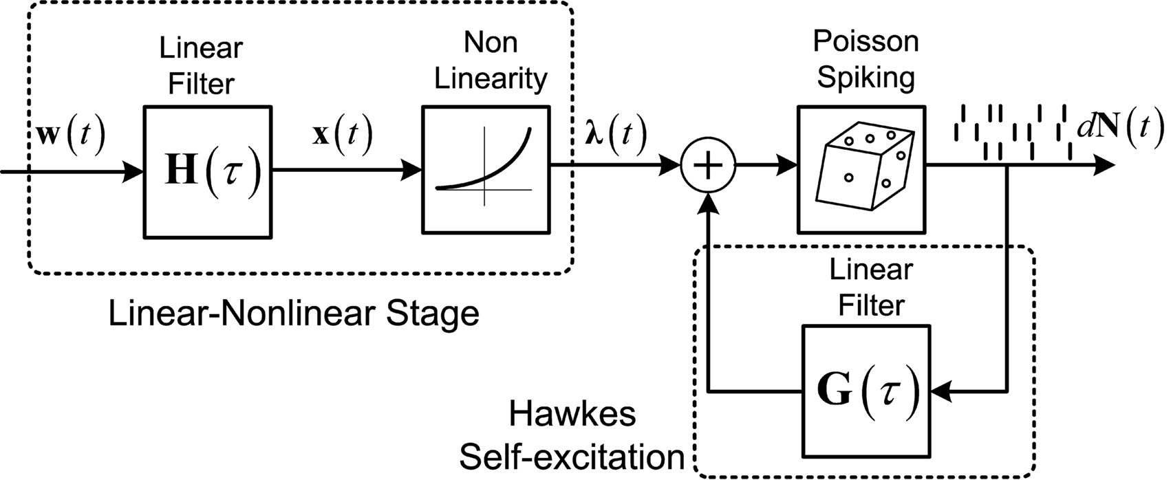
Figure 1. Linear–Non-linear-Hawkes model diagram. White multivariate Gaussian noise w(t) passes through a Linear–Non-linear cascade, resulting in an exogenous input, λ(t), to the Hawkes model. By setting the Hawkes self- and mutual-excitation feedback filter to equal zero we remain with a multivariate Linear–Non-linear-Poisson (LNP) model. By setting λ(t) = λ we get the Hawkes model.

Methods

In this section we begin by defining the Hawkes model, recalling its auto-correlation structure and then generalizing to multivariate (mutually exciting) non-homogeneous Hawkes model of point processes. Next, we propose a method for the solution of the resulting equations, and for the estimation of the different parameters of the model. In the final subsection the experimental methods of stimulation and data acquisition are presented.

Theoretical Background

Let us consider the intensity of a self-exciting point process to be defined by the following expression:

Here, the instantaneous firing intensity μ(t) is the exogenous input λ summed together with multiple shifted replicas of the self-excitation kernel g(t). The kernels are causal (g(t) = 0, t < 0), and t_k represents all the past spike-times. For technical reasons we will write the expression using the Stieltjes integral:

where N(t) is the counting process (number of spikes up to time t). The sum term in Eq. 1 is now replaced by a convolution of the spiking history with a linear kernel. The mean firing rate (denoted throughout the paper by 〈dN〉) of this point process is given by:

Resulting in:

The stability (and stationarity) condition for this model can easily be inferred from this equation. An expression for the auto-covariance function of such a point process was derived in Hawkes (1971a), and we will briefly review here the main results (adapted from his auto-covariance notation into auto-correlation function notation used here for simplicity). We will distinguish between two different auto-correlation functions, the first:

which has a delta function singularity 〈dN〉·δ(τ) at τ = 0 due to the nature of point processes, and the second:

from which this singularity was subtracted.

Using these definitions we get the following integral equation for the auto correlation of the output point process of the Hawkes model:

This equation can be solved numerically (Mayers, 1962) or by using Wiener–Hopf related techniques (Noble, 1958; Hawkes, 1971b).

Similarly, Hawkes (1971a) generalized this solution (Eqs 4 and 7) to multivariate mutually exciting point processes by using matrix notation. The intensity of mutually exciting process becomes:

with mean firing rates:

and the cross-correlation matrix as a solution of:

The Linear–Non-linear-Hawkes model and its correlations

Let us now consider a more general case of a non-homogeneous Hawkes model, where the exogenous input λ(t) can be a time-varying (stationary) process:

For example, this class of models includes the important special case (Figure 1) where λ(t) is itself a non-negative stationary random process generated by a Linear–Non-linear cascade acting on a Gaussian process input (possibly a stimulus). Note the difference between the proposed linear–non-linear-Hawkes (LNH) model and the GLM-type models, in which the feedback term is summed with the x(t) and not with the λ(t) (according to the notation in Figure 1). This effectively changes the locus of the non-linearity present in the model and affects the model’s properties and analytical tractability.

The mean firing rate of this point process can, in general, be found in a similar way as in Eqs 3 and 4:

Next, the auto-correlation function R_dN(τ) of this process can be derived using a similar procedure to the derivation of Eq. 7 (the detailed derivation can be found in Section “Correlation Structure of the LNH Model” of Appendix). This time, the auto-correlation function is governed by two coupled integral equations:

These two equations provide the solution for the output auto-correlation function R_dN(τ) and for the cross-correlation between the exogenous input λ(t) and the point process whose intensity is defined by Eq. 11. Here, the input auto-correlation function R_λ(τ) and the self-exciting kernel g(τ) serve as given parameters (see also Identification of the LNH Model).

Equations 12 and 13 can be further generalized to a multivariate case (mutually exciting point processes), and be written using the matrix notation:

Note that for constant λ these equations are reduced to Eqs 9 and 10.

Identification of the LNH Model

The equations for the correlation structure of a single self-exciting point process and multivariate mutually exciting point processes (Eqs 13 and 14 respectively) can be solved numerically by switching from continuous time integral notation to discrete time matrix notation, and consequently performing matrix calculations. The integration operations in the Eqs 13 and 14 are thus converted to matrix multiplication operations. This allows a simple and straightforward way to solve the equations for the output correlation structure. Here, we only briefly present the main results. All the detailed explanations on the notation used, on how the appropriate matrices and vectors are built, and how the equations are solved in both single- and multi-channel cases can be found in Section “Solution of the Integral Equations” of Appendix. Using the new notation the output correlation is estimated by:

where are block column vectors that represent the sampled versions of the correlations R_dN(τ), R_λ(τ), R_λdN(τ), and the feedback kernel G(τ). Block matrices and are built from G(τ), and is the unity matrix of appropriate dimensions (see also Solution of the Integral Equations of Appendix). The generalized Hawkes model has three different sets of parameters – the input correlation structure R_λ(τ), the output correlation structure R_dN(τ), and the Hawkes feedback kernel G(τ). Thus, in addition to the forward problem solution presented in Eq. 15, there are three other possible basic scenarios for the identification of the different parts of the proposed generalized Hawkes model from the correlation structure of the observed spike train(s).

In the first scenario we are interested in the estimation of the input correlation structure, given the output correlation structure R_dN(τ) and the Hawkes kernel G(τ). By using the aforementioned matrix notation the solution can be achieved in a straightforward manner, akin to the forward problem:

After R_λ(τ)is estimated one can proceed, if interested, with the estimation of an LN cascade model for this correlation structure by applying the correlation pre-distortion procedures developed and detailed in (Krumin and Shoham, 2009) and (Krumin and Shoham, 2010). Estimation of the Linear–Non-linear cascade model, in addition to the connectivity kernels G(τ), can provide additional insights about the stimulus-driven neural activity.

The second possible scenario is to estimate the Hawkes kernels when the output and the input correlation structures are known (see, e.g., Figure 3B). Here, once again, we can use the advantage of the same matrix notation (block column vector and block matrix represent the R_λdN(τ) and R_dN(τ) correlation functions, respectively) and solve the following equations in an iterative manner to estimate G(τ):

where stands for the block diagonal matrix with diag (〈dN〉) as its block elements on the main diagonal.

The iterative solution of this set of equations is explained in detail in Section “Solution of the Integral Equations” of Appendix, Eq. A23.

The third possible scenario is to estimate both the kernels G(τ) and the input correlation structure R_λ(τ), given only the output correlation structure R_dN(τ). In general, this problem is not well-posed and does not have a unique solution, and additional application-driven constraints on the structure of G(τ) and/or R_λ(τ) should be considered. We will leave additional discussion on the uniqueness of the solution to the results (see Application to Neural Spike Trains – Single Cells) and in Sections “Discussion.”

Refractoriness and strong inhibitory connections

In general, the connectivity between the different units (G(τ) feedback terms in the Hawkes model) is not limited to non-negative values. Hence, the firing intensity μ(t) defined in Eqs 1 or 8 can occasionally become negative. However, the analytical derivations for the output mean rate and correlation structure are based on the assumption that μ(t) is non-negative for all t. The violation of this assumption results in a discrepancy between the actual and the analytical results. Simulation of the estimated LNH model [while using the effective firing intensity μ_eff(t) = max{μ(t), 0}] yields output spike trains with a correlation structure that is different from the desired output correlation structure R_dN(τ) (used for the estimation of the model parameters). To address this issue an additional procedure was developed for the estimation of the actual feedback kernel g(τ) from the input and the output correlations (R_λ(τ) and R_dN(λ), respectively). The procedure is summarized in the following algorithm:

1. Estimate initial g(τ) from R_λ(τ) and R_dN(λ) by solving Eq. 13 (in its matrix form of Eq. 17).

2. Simulate a Hawkes point process using the original input correlation R_λ(τ) and the estimated kernel g(τ). Use μ_eff(t) = max{μ(t), 0}.

3. Estimate the output correlation of the simulated spike train. The violation of the μ(t) ≥ 0 assumption will result in a difference between the desired (R_dN(τ)) and the estimated output correlation structures.

4. Use the estimated instead of the input correlation R_λ(τ) in the Eq. 13 to estimate the kernel Δg(τ). The output correlation that should be used is the desired R_dN(τ) throughout the iterative solution, only the input correlation R_λ(τ) changes from iteration to iteration.

5. Update g(τ) ← g(τ) + α·Δg(τ). The scalar α ≤ 1 is used for controlling the speed and/or smoothness of the convergence. In Section “Application to Neural Spike Trains – Single Cells” we have used a relatively small α = 0.1 to ensure smooth convergence to the solution.

6. Loop through steps 2–5 until the actual of the simulated spike train converges to the desired R_dN(τ).

The above procedure uses the difference between the model-based (simulated) and the desired (data-estimated) correlation structures of the output spike trains to systematically update the feedback kernel g(τ) until the difference between these two correlation structures becomes small enough. The resulting model allows to relax the assumption of μ(t) ≥ 0 and to use μ_eff(t) = max{μ(t), 0} instead.

Experimental Methods

Retina preparation

Animal experiments and procedures were approved by the Institutional Animal Care Committee at the Technion – Israel Institute of Technology and were in accordance with the NIH Guide for the Care and Use of Laboratory Animals. Six-week-old wild type mice (C57/BL) were euthanized using CO₂ and then decapitated. Eyes were enucleated and immersed in Ringer’s solution containing (in mM): NaCl, 124; KCl, 2.5; CaCl₂, 2; MgCl₂, 2; NaHCO₃, 26; NaH₂PO₄, 1.25; and Glucose, 22 (pH 7.35–7.4 with 95% O₂ and 5% CO₂ at RT). An incision was made at the ora serrata using a scalpel and the anterior chamber of the eye was separated from the posterior chamber cutting along the ora serrata with fine scissors. The lens was removed and the retina was gently cleaned of the remaining vitreous. Retinal tissue was isolated from the retinal pigmented epithelium. Three radial cuts were made and the isolated retina was flattened with the retinal ganglion cells facing the multi electrode array (MEA). During the experiment the retina was continuously perfused with oxygenated Ringer’s solution.

Electrophysiology

The retina was stimulated by wide-field intensity-modulated light flashes using a DLP-based projector. The stimulus intensities were normally distributed and updated at the rate of 60 Hz. Resulting activity was recorded using 60-channel MEA with 10 μm diameter, planar electrodes spaced at 100 μm. The data was acquired with custom written data acquisition software using Matlab 7.5.0 data acquisition toolbox.

Results

Simulation Studies

We performed a number of simulation studies to validate the methods proposed for the solution of the integral Eqs 13 and 14.

In Figures 2A–C the forward model solution by the Eq. 15 is compared to the auto-correlation function estimated from single simulated point processes with different self-excitation kernels, g(τ), under two different conditions – constant input λ (pure Hawkes model), or time-varying input λ(t) with an exponentially shaped auto-correlation function (LNH model). In Figure 2D an example of a bivariate case is presented with a more complex correlation structure of the input λ(t) and a set of self- and mutually exciting kernels G(τ).

FIGURE 2

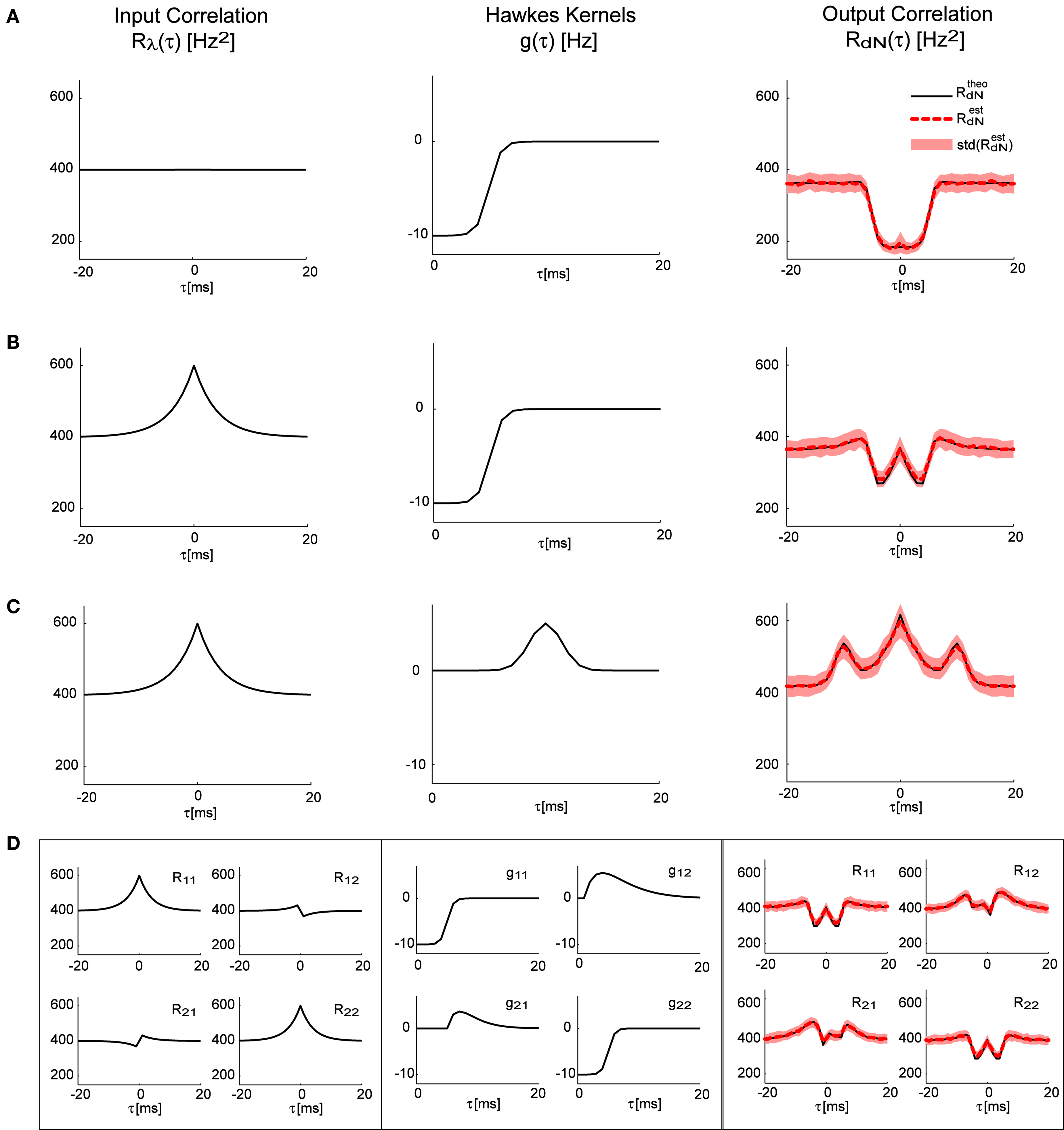
Figure 2. Correlation structure of the homogeneous and inhomogeneous Hawkes models can be accurately predicted. Predicted theoretical correlation structure is compared to the correlation structure estimated from simulated point processes in several cases: (A) Constant λ and a refractory period-like self-exciting kernel g(τ). (B) Same as in (A), but with time-varying λ(t) that has an exponentially shaped auto-correlation function. (C) Similar to (B), but with a different self-excitation kernel g(τ). (D) Bivariate mutually exciting point processes driven by time-varying exogenous inputs with complex correlation structure. Mean values and standard deviations of the estimators were calculated from 100 simulations (each 10 min long) of corresponding Hawkes models.

As can be seen in all of these examples, the analytically predicted correlation functions had a near-perfect match with the mean correlation functions of the simulated spike trains (correlation coefficient ≥0.99). Individual correlation functions calculated from 10-min traces were more noisy, thus the forward analytical prediction vs. simulation correlation coefficients for single traces were significantly lower: 0.83 ± 0.06.

Figure 3A shows the result of applying the “scenario I” solution (Eq. 16) to spike trains generated by the model presented in Figure 2D; the mean identified input correlations have an excellent match with the ones used for generating the data (correlation coefficients: 0.99 and 0.92 respectively for the auto- and cross-correlations).

FIGURE 3

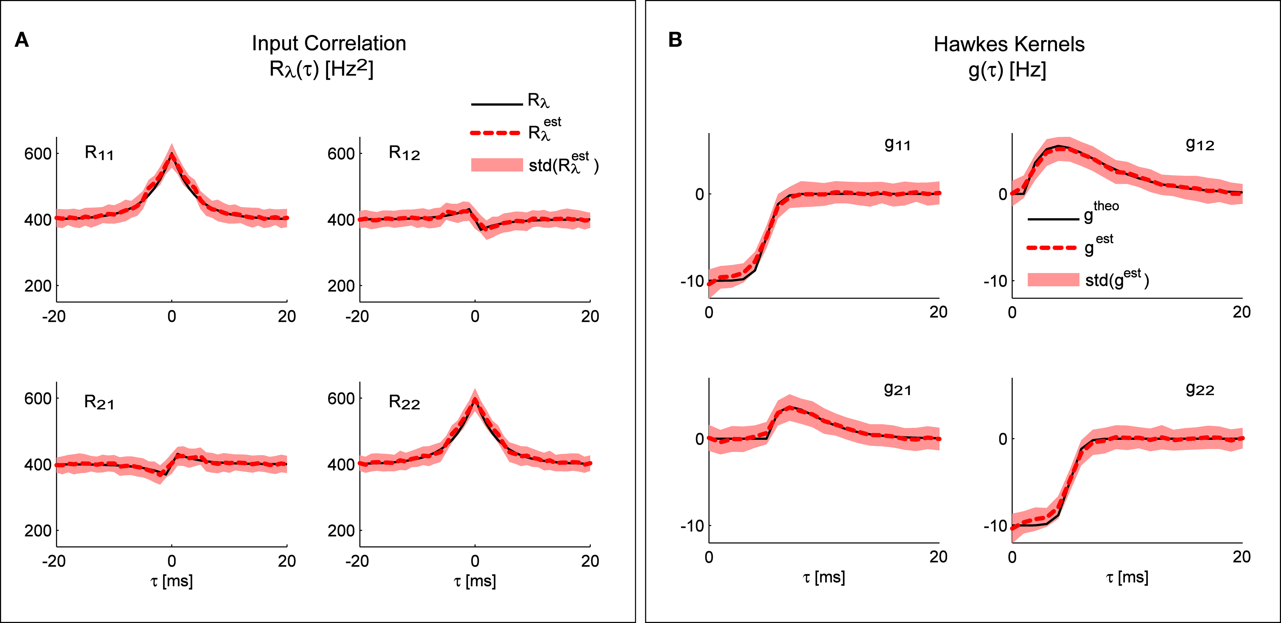
Figure 3. System identification. Any of the three different parts of the system can be identified from the other two. (A) Comparison of the input correlation structure estimated from the simulated point processes and the real values used in the simulation. (B) Hawkes kernels estimated from the simulated point processes and input correlation structure are compared to their real value used for the simulation. Mean values and standard deviations of the estimators were calculated from 100 simulations (each 10 min long) of the bivariate inhomogeneous Hawkes models from Figure 2D.

Figure 3B shows the result of applying the “scenario II” solution (Eq. 17) to spike trains generated by the model presented in Figure 2D; the mean identified kernels greatly match the ones used in generating the data (correlation coefficients >0.99 for all kernels.

Application to Neural Spike Trains – Single Cells

Next, we applied the method on the data recorded from the retina (see Methods for the experimental protocol). We started by analyzing the spike trains using reverse-correlation techniques (Ringach and Shapley, 2004) based on a feed-forward Linear–Non-linear–Poisson (LNP) model. The LNP-based estimates of the linear filter, and the static non-linearity (Figure 4A) were further used for the calculation of the expected output auto-correlation function of the estimated LNP model. This LNP-based output auto-correlation function was found to be noticeably different from the actual auto-correlation function of the measured spike trains (Figure 4B).

FIGURE 4

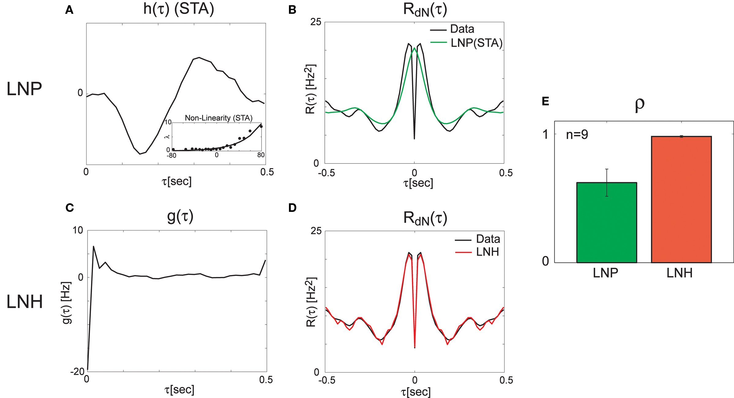
Figure 4. Linear–non-linear-Hawkes and LNP model fits to single-unit retinal neural spike train auto-correlations. Single-unit recordings from mouse retinal ganglion cells were analyzed using the LNP and the LNH model-based approaches with the LNH model succeeding to explain the spike trains’ correlations much better than the LNP model. (A) Linear filter h(τ) and the non-linearity estimated using reverse-correlation approach (spike triggered average). (B) The expected output auto-correlation function of the LNP model calculated from the parameters in (A) does not fit the actual auto-correlation function of the spike train well. (C) The self-excitation kernel g(τ) of the LNH model shows strong refractoriness that cannot be explained by the LNP model. (D) The LNH model output auto-correlation precisely fits the actual spike train auto-correlation measured from the data. (E) The correlation coefficients between the model and the actual output auto-correlation functions are significantly (p = 0.005) higher for the LNH model (with mean ± SE of ρ_LNP = 0.62 ± 0.11 and ρ_LNH = 0.98 ± 0.01, n = 9).

This LN cascade was then used for generating the input (λ(t) in Figure 1) to the Hawkes feedback stage of the LNH model. The auto-correlation function of λ(t) is exactly that of the LNP model’s output estimated previously and found inconsistent with the real recordings. Now, the input auto-correlation function R_λ(τ) was used together with the measured output auto-correlation function R_dN(τ) to estimate the Hawkes feedback kernel g(τ) (Figure 4C) from Eq. 13 (including the procedure described in the Refractoriness and Strong Inhibitory Connections). Interestingly, the output auto-correlation function of the newly estimated LNH model (as measured from the simulated spike trains) was in excellent agreement with the auto-correlation function of the actual neural data (Figure 4D). The addition of the linear Hawkes feedback stage to the classical feed-forward LNP model proved beneficial to the model’s capability of explaining more complex spike train correlation structures of real neural recordings (Figure 4E).

Finally, we validated that the improved fit of the LNH model to the data compared with the LNP model, does not result from a model overfitting due to the larger number of parameters in the LNH model. For each unit, we computed an LN-Hawkes for a different data set from the same unit (Gaussian distribution, different mean intensity). Next, we simulated an output spike train using a “hybrid” LNH model (“original” LN model + “new” feedback kernel g(τ)), and estimated its correlation function. This output correlation function was compared to the correlation function of the original data by calculating the correlation coefficient between the two functions ρ_LNH. This procedure was applied to the nine units in our data set where the mean firing rates were >2 Hz. In eight out of these nine units the hybrid LNH model provided considerably better fits to the output correlation function than the corresponding LNP model, providing in those cases an average improvement of 〈Δρ〉 = 〈ρ_LNH − ρ_LNP〉 = 0.19 with 〈Δρ〉/〈ρ_LNP〉 = 30%. Note that this procedure is over-conservative, since there is no guarantee that kernels calculated for different input stimulus ensembles will be the same or conversely, that neural models will generalize across different stimulus ensembles.

Discussion

In this paper, we extended previous work on the correlation-based simulation, identification and analysis of multi-channel spike train models with a feed-forward Linear–Non-linear (LN) stage driven by Gaussian process inputs (Krumin and Shoham, 2009; Krumin et al., 2010), by allowing the non-negative process to drive a feedback stage in the form of a multi-channel Hawkes process. The move from doubly stochastic Poisson (Cox) models in our previous work to doubly stochastic Hawkes models employed here vastly expands the range of realizable correlation structures, thus relaxing the main limitation of the previous results, and allowing for a superior, excellent fit (ρ ≃ 0.98) of the auto-correlation structures of spike trains recorded from real visually driven retinal ganglion cells. At the same time, it preserves the analytical tractability and closed-form correspondence between model parameters and the second-order statistical properties of the output spike trains, and thus, essentially, all of the advantages and potential applications of the general model-based correlation framework, which was limited, thus far, to feed-forward models. These currently include the synthetic generation of spike trains with a pre-defined correlation structure (Brette, 2009; Krumin and Shoham, 2009; Macke et al., 2009; Gutnisky and Josic, 2010; Tchumatchenko et al., 2010), “blind” correlation-based identification of single-neuron encoding models (Krumin et al., 2010), the compact representation of multi-channel spike trains in terms of multivariate auto-regressive processes and the framework of causality (Granger) analysis (Nykamp, 2007; Krumin and Shoham, 2010). As noted above, the LNH model is related to the commonly used GLM model, with the LNH feedback kernels paralleling the GLM history terms. Both ways of altering the underlying feed-forward LNP model lead to more flexible models capable of fitting more complex correlation structures, but the preferred fitting procedures for the two models differ: the GLM model is typically fit using a maximum likelihood approach, but this does not suit the LNH model (due to possible zero firing rates), where a method of moments (like the one introduced here) is more appropriate for the estimation of the linear kernels. A systematic study on the differences between the statistical properties of the two approaches falls beyond the scope of the current manuscript.

The model and analysis presented here also provide a new context and results to a significant body of related previous work on the second-order statistics of Hawkes models, which we will now review very briefly. The basic properties of the output correlation structure and the spectrum of a univariate self-exciting and a multivariate mutually exciting linear point process model without an exogenous drive were derived in the original works of Hawkes (1971a,b) using the linear representation of this process (Eq. 2). Brillinger (1975) also analyzes linear point process models and uses spectral estimators for the kernels, which he applies to the analysis of synaptic connections (Brillinger et al., 1976). Bremaud and Massoulie (2002) and Daley and Vere-Jones (2003) (exercise 8.3.4) present expressions for the output spectrum of a univariate Hawkes model excited by an exogenous correlated point process derived using an alternative, cluster process representation of the Hawkes process:

where and represent the respective spectra of dN(t), λ(t), g(t). Our derivation in the Section “Methods” and “Correlation Structure of the LNH Model” of Appendix focused on expressions for the correlation structure of exogenously driven Hawkes process and was based on the linear representation, similar to Hawkes (1971a). Adding the exogenous input introduces a new term into the Hawkes integral Eq. 10, and a second integral equation for the cross-covariance term between the exogenous input and the output spike trains R_λdN(τ). The parameters of these generalized models, i.e., the kernels G(τ) and/or the input correlation structure R_λ(τ), can be directly estimated from the output process correlation structure using an iterative application of this set of equations, as illustrated in Section “Results,” or they could, alternatively, be estimated from the spectral expressions.

We next turn to discuss certain limitations of the proposed framework. First, the analytical equations for the auto-correlation structure of the point processes (Eqs 7, 10, 13, and 14) are exactly true under the assumption μ(t) ≥ 0 (Eqs 2, 8, and 11) or when the stochastic intensity is always non-negative. These exact results could also provide an excellent agreement to many practical cases wherein the self-exciting Hawkes kernel g(τ) is only weakly negative (e.g., Figure 2), leading in such cases to slight systematic deviations at “negative” peaks. In cases of strong refractoriness or other inhibitory interactions, g(τ) becomes strongly negative, and the rectification of the stochastic intensity around zero leads to strong deviations from the assumptions underlying Eqs 7 and 13. For such cases we introduced an intuitive iterative procedure for computing g(τ) (see Refractoriness and Strong Inhibitory Connections), and it is likely that related alternatives are also possible. Although the convergence of this procedure is not proven, in practice, it was capable of estimating kernels for real neural spike trains that not only dramatically improved the auto-correlation fits relative to LNP cascades, but also generalized across different stimulus ensembles (a very conservative cross-validation test). Second, we have not addressed the important but complex issue of uniqueness of the different identification problems encountered here. Interestingly, in the examples we have examined, an excellent match was found, in practice, between the Hawkes kernels and their estimates (Figure 3B), although we are not aware of any guarantees of uniqueness here (these may perhaps be related to the nature of point processes). In the more general problem where both are simultaneously estimated, it seems obvious that unique solutions can only be obtained by imposing additional constraints on the solutions (i.e., degree of smoothness and/or sparseness). In section “Application to Neural Spike Trains – Single Cells” we presented an example of the “scenario III”-type problem, where only the output correlation structure is actually observable. In this example we used additional application-driven constraints on the input correlation structure R_λ(τ) to infer the feedback kernels G(τ). Interestingly, the exact same “scenario III”-type framework can be used for generating synthetic spike trains with a controlled correlation structure. This application will benefit from using the LNH feedback model by harnessing the capability of generating spike trains with a much richer ensemble of possible correlation structures in comparison with the feed-forward-only models like LNP. Additionally, once is determined there is an additional level of non-uniqueness in the determination of the underlying LN structure, which can also be overcome by imposing constraints (e.g., a minimum phase constraint (Krumin et al., 2010)).

When considering the broader relevance of this work, and the directions to which it may develop in the future, it is worth noting that some of the most fundamental and widely applied tools for the identification of systems rely on the use of second-order statistical properties (Ljung, 1999) (correlation or spectral). The increasing arsenal of tools for identifying spike train models from their correlations, rather than from their full observed realizations could form a welcome bridge between “classical” signal processing ideas and tools and the field of neural spike train analysis.

Conflict of Interest Statement

The authors declare that the research was conducted in the absence of any commercial or financial relationships that could be construed as a potential conflict of interest.

Acknowledgments

This work was supported by Israeli Science Foundation grant #1248/06 and European Research Council starting grant #211055. We thank A. Tankus and the two anonymous reviewers for their comments on the manuscript.

References

Bremaud, P., and Massoulie, L. (2002). Power spectra of general shot noises and Hawkes point processes with a random excitation. Adv. Appl. Probab. 34, 205–222.

CrossRef Full Text

Brette, R. (2009). Generation of correlated spike trains. Neural. Comput. 21, 188–215.

Pubmed Abstract | Pubmed Full Text | CrossRef Full Text

Brillinger, D. (1988). Maximum likelihood analysis of spike trains of interacting nerve cells. Biol. Cybern. 59, 189–200.

Pubmed Abstract | Pubmed Full Text | CrossRef Full Text

Brillinger, D. R. (1975). The identification of point process systems. Ann. Probab. 3, 909–924.

CrossRef Full Text

Brillinger, D. R., Bryant, H. L., and Segundo, J. P. (1976). Identification of synaptic interactions. Biol. Cybern. 22, 213–228.

Pubmed Abstract | Pubmed Full Text | CrossRef Full Text

Brown, E. N., Kass, R. E., and Mitra, P. P. (2004). Multiple neural spike train data analysis: state-of-the-art and future challenges. Nat. Neurosci. 7, 456–461.

Pubmed Abstract | Pubmed Full Text | CrossRef Full Text

Cardanobile, S., and Rotter, S. (2010). Multiplicatively interacting point processes and applications to neural modeling. J. Comput. Neurosci. 28, 267–284.

Pubmed Abstract | Pubmed Full Text | CrossRef Full Text

Chichilnisky, E. J. (2001). A simple white noise analysis of neuronal light responses. Network 12, 199–213.

Pubmed Abstract | Pubmed Full Text

Chornoboy, E., Schramm, L., and Karr, A. (1988). Maximum likelihood identification of neural point process systems. Biol. Cybern. 59, 265–275.

Pubmed Abstract | Pubmed Full Text | CrossRef Full Text

Daley, D. J., and Vere-Jones, D. (2003). An Introduction to the Theory of Point Processes, Vol. 1. New York: Springer.

Granger, C. W. J. (1969). Investigating causal relations by econometric models and cross-spectral methods. Econometrica 37, 424–438.

CrossRef Full Text

Gutnisky, D. A., and Josic, K. (2010). Generation of spatio-temporally correlated spike-trains and local-field potentials using a multivariate autoregressive process. J. Neurophysiol. 103, 2912–2930.

Pubmed Abstract | Pubmed Full Text | CrossRef Full Text

Hawkes, A. G. (1971a). Spectra of some self-exciting and mutually exciting point processes. Biometrika 58, 83–90.

CrossRef Full Text

Hawkes, A. G. (1971b). Point spectra of some mutually exciting point processes. J. R. Stat. Soc. Series B Methodol. 33, 438–443.

Johnson, D. H. (1996). Point process models of single-neuron discharges. J. Comput. Neurosci. 3, 275–299.

Pubmed Abstract | Pubmed Full Text | CrossRef Full Text

Kailath, T., Sayed, A. H., and Hassibi, B. (2000). Linear Estimation. Upper Saddle River, NJ: Prentice Hall.

Krumin, M., Shimron, A., and Shoham, S. (2010). Correlation-distortion based identification of Linear-Nonlinear-Poisson models. J. Comput. Neurosci. 29, 301–308.

Pubmed Abstract | Pubmed Full Text | CrossRef Full Text

Krumin, M., and Shoham, S. (2009). Generation of spike trains with controlled auto- and cross-correlation functions. Neural. Comput. 21, 1642–1664.

Pubmed Abstract | Pubmed Full Text | CrossRef Full Text

Krumin, M., and Shoham, S. (2010). Multivariate auto-regressive modeling and granger causality analysis of multiple spike trains. Computat. Intell. Neurosci. 2010, Article ID 752428.

Ljung, L. (1999). System Identification – Theory for the User, 2nd Edn. Upper Saddle River, NJ: Prentice Hall PTR.

Macke, J. H., Berens, P., Ecker, A. S., Tolias, A. S., and Bethge, M. (2009). Generating spike trains with specified correlation coefficients. Neural. Comput. 21, 397–423.

Pubmed Abstract | Pubmed Full Text | CrossRef Full Text

Mayers, D. F. (1962). “Part II. Integral equations, Chapters 11–14,” in Numerical Solution of Ordinary and Partial Differential Equations, ed. L. Fox (London: Pergamon), 145–183.

Noble, B. (1958). Methods Based on the Wiener-Hopf Technique. London: Pergamon.

Nykamp, D. Q. (2007). A mathematical framework for inferring connectivity in probabilistic neuronal networks. Math. Biosci. 205, 204–251.

Pubmed Abstract | Pubmed Full Text | CrossRef Full Text

Paninski, L., Pillow, J., and Lewi, J. (2007). Statistical models for neural encoding, decoding, and optimal stimulus design. Prog. Brain Res. 165, 493–507.

Pubmed Abstract | Pubmed Full Text | CrossRef Full Text

Paninski, L., Shoham, S., Fellows, M. R., Hatsopoulos, N. G., and Donoghue, J. P. (2004). Superlinear population encoding of dynamic hand trajectory in primary motor cortex. J. Neurosci. 24, 8551–8561.

Pubmed Abstract | Pubmed Full Text | CrossRef Full Text

Pillow, J. W., Shlens, J., Paninski, L., Sher, A., Litke, A. M., Chichilnisky, E. J., and Simoncelli, E. P. (2008). Spatio-temporal correlations and visual signalling in a complete neuronal population. Nature 454, 995–999.

Pubmed Abstract | Pubmed Full Text | CrossRef Full Text

Ringach, D., and Shapley, R. (2004). Reverse correlation in neurophysiology. Cogn. Sci. 28, 147–166.

CrossRef Full Text

Shoham, S., Paninski, L. M., Fellows, M. R., Hatsopoulos, N. G., Donoghue, J. P., and Normann, R. A. (2005). Statistical encoding model for a primary motor cortical brain-machine interface. IEEE Trans. Biomed. Eng. 52, 1312–1322.

Pubmed Abstract | Pubmed Full Text | CrossRef Full Text

Stevenson, I. H., Rebesco, J. M., Miller, L. E., and Koerding, K. P. (2008). Inferring functional connections between neurons. Curr. Opin. Neurobiol. 18, 582–588.

Pubmed Abstract | Pubmed Full Text | CrossRef Full Text

Tchumatchenko, T., Malyshev, A., Geisel, T., Volgushev, M., and Wolf, F. (2010). Correlations and synchrony in threshold neuron models. Phys. Rev. Lett. 104, 058102.

Pubmed Abstract | Pubmed Full Text | CrossRef Full Text

Toyoizumi, T., Rad, K. R., and Paninski, L. (2009). Mean-field approximations for coupled populations of generalized linear model spiking neurons with Markov refractoriness. Neural. Comput. 21, 1203–1243.

Pubmed Abstract | Pubmed Full Text | CrossRef Full Text