Elemental spiking neuron model for reproducing diverse firing patterns and predicting precise firing times

Introduction

A mathematical model of a single-neuron that is capable of accurately reproducing diverse spiking behaviors of biological neurons is required for simulating real neuronal circuitry (Diesmann et al., 1999; Izhikevich, 2004; McIntyre et al., 2004; Markram, 2006; Brette et al., 2007; Gewaltig and Diesmann, 2007; Izhikevich and Edelman, 2008; Plesser and Diesmann, 2009; Rossant et al., 2011). The leaky integrate-and-fire (LIF) neuron models, which had been regarded as a simple toy model of a single-neuron, have significantly developed in the direction of quantitatively analyzing electrical properties of real neurons by enhancing their adaptability to data (for a review of the LIF model, see Burkitt, 2006). Spike response models (SRMs; Gerstner and van Hemmen, 1992; Gerstner, 1995) based on linear integration of input currents have been successful in not only reproducing the data but also predicting the precise spike times for new inputs (Kistler et al., 1997; Gerstner and Kistler, 2002; Jolivet et al., 2004, 2006; Kobayashi and Shinomoto, 2007). Furthermore, non-linearity has been introduced to the model in a systematic manner and its suitability has been tested in typical neurons (Fourcaud-Trocmé et al., 2003; Izhikevich, 2003; Brette and Gerstner, 2005; Badel et al., 2008).

Given the idea that a good spiking neuron model can predict neuronal firings for new fluctuating inputs, the International Competition on Quantitative Single-Neuron Modeling was organized [International Neuroinformatics Coordinating Facility (INCF), 2009]. In the competition, spike neuron models were assessed based on their quantitative performance in accurately predicting spike times (Mainen and Sejnowski, 1995; Jolivet et al., 2008; Gerstner and Naud, 2009). The simplistic integrate-and-fire models described above displayed higher performance than the complicated biophysical neuron models of Hodgkin–Huxley type (Hodgkin and Huxley, 1952). Among the winning models, the multi-timescale adaptive threshold (MAT) model (Kobayashi et al., 2009; Shinomoto, 2010) performed best in prediction. This model was one of the simplest models and is based on the linear leaky integration of input currents with a moving threshold.

The criterion for assessing the spiking neuron model is not unique; in addition to quantitative reproducibility, neuron models are expected to possess the ability to manifest various firing patterns of biological neurons, as represented by the 20 different firing responses to transient currents demonstrated by Izhikevich (2004). In this respect, the complicated biophysical Hodgkin–Huxley models are capable of representing such a variety of firing responses, whereas the simple LIF models (including the MAT model) are incapable of reproducing diverse responses. Izhikevich (2003) proposed a simplistic non-linear model that can express this diversity. More recently, Mihalas and Niebur (2009) proposed a linear integrate-and-fire model that can produce a fairly rich variety of firing responses.

In this study, we apply improvements to the MAT model so that it is able to handle the 20 qualitative firing responses introduced by Izhikevich (collectively known as Izhikevich’s table), including inhibitory rebound spiking and resonate spiking. Our improved MAT model must not negatively impact the strong adaptability and predictability that the original MAT model possesses. Here the difficulty is that any model tends to be intractable when large degrees of freedom for diversity are added. In accordance with the wisdom of Occam’s razor, we refrain from defining a large number of parameters; instead, we augment only one parameter, and then observe whether the model becomes both capable of covering various firing patterns while maintaining its strong quantitative predictive performance.

In this paper, we first provide a full analysis of the dynamics of the original MAT model, and describe our enhanced model by introducing the voltage dependent term. Next, we examine the model to determine whether it is capable of reproducing the entire set of qualitative features. Finally, we examine the augmented model to determine whether it possesses the ability to precisely predict spike times of biological neurons.

Dynamic Characteristics of the Original MAT Model

Before extending the MAT model, we first analyze the dynamic characteristics of the original MAT model, which consists of two parts: the non-resetting leaky integrator and the MAT (Kobayashi et al., 2009). Figure 1 illustrates the dynamics of the MAT model.

FIGURE 1

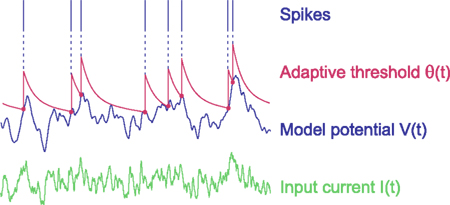
Figure 1. Dynamics of the multi-timescale adaptive threshold (MAT) model. The model potential V(t) (blue) is obtained from input current I(t) (green) with the non-resetting leaky integration given in Eq. 1. If the model potential hits threshold θ(t) (red), the model assumes a spike and increases the threshold. The adaptive threshold θ(t) decays toward resting value ω with multiple timescales according to Eqs 2 and 3.

The dynamics of the non-resetting leaky integrator is given by

where V(t) and I(t) are the model potential and input current, and τ_m and R are parameters representing the leak time constant and input resistance, respectively. The model assumes a spike when V(t) reaches a threshold value indicated by θ(t). In this model, V(t) is not reset as in the standard LIF model (Stein, 1965, 1967), but instead, threshold θ(t) is increased, and then decays toward its resting value. In standard adaptive threshold models, the spike threshold θ(t) decays with a single exponential function (Geisler and Goldberg, 1966; Brandman and Nelson, 2002; Chacron et al., 2003), but the present model contains multiple exponential decays, given by

where t_k is the kth spike time, L is the number of threshold time constants, τ_j is the jth time constant, α_j is the weight of the jth time constant, and ω is the resting value. In addition, to avoid singular bursting, the neuron is not allowed to fire within an absolute refractory period τ_R even when the membrane potential exceeds the threshold. If the membrane potential lies above the threshold after the period τ_R, the model assumes another spike.

The model is therefore fully specified by the parameters {τ_m, R, τ_R, τ_j, α_j, (j = 1, 2,…, L), ω}. We inherit many of the parameter values adopted in the original MAT model of L = 2, as R = 50 MΩ, τ_R = 2 ms, τ₁ = 10 ms, and τ₂ = 200 ms, which were determined using experimental data obtained by current injection experiments on cortical neurons, including regular-spiking (RS), intrinsic-bursting (IB), and fast-spiking (FS) neurons (Kobayashi et al., 2009). Here, the multiple timescales are regarded as respectively expressing different biological ionic currents, such that 10 ms represents fast transient Na⁺ current and delayed rectifier K⁺ current, and 200 ms represents non-inactivating K⁺ current, hyperpolarization-activated cation current, and Ca²⁺-dependent K⁺ current (Koch, 1999; Hille, 2001). The only one parameter that we modified from the original MAT model is the membrane time constant; we changed it from τ_m = 5 to 10 ms. This is because the time constant fitted to the present data turned out to be 11.7 ms, the original time constant 5 ms is too small compared to the widely accepted range of membrane time constant 10–20 ms (McCormick et al., 1985; Yang et al., 1996), and the spike time prediction performed with τ_m = 10 ms gave rise to the highest predictive performance among the choices of 5, 10, 11.7, 15, and 20 ms.

The MAT model is capable of reproducing a variety of spike responses manifested by a broad class of cortical neurons, including RS, IB, and FS neurons. Furthermore, the MAT model is capable of demonstrating repeated burst firing called “chattering” (CH; Gray and McCormick, 1996). To examine the basic capability of the model in expressing a wide variety of qualitative firing features, we first use bifurcation theory (Hoppensteadt and Izhikevich, 1997) to investigate the firing response of the original MAT model given a constant current injection.

Using bifurcation analysis, we find that the model parameter space can be divided into domains in which the model exhibits qualitatively different dynamic behavior, as represented by type I or II excitability, which is defined according to whether the frequency–current (f–I) relationship is continuous or discontinuous at the threshold current, respectively (Hodgkin, 1948; Rinzel and Ermentrout, 1989), and bursting (Izhikevich, 2007). Figure 2 depicts the allocation of the three domains on a plane of parameters α₁ and α₂, which is obtained by sectioning a three-dimensional parameter space at a given residual parameter ω.

FIGURE 2

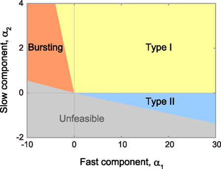
Figure 2. Phase diagram in the α₁–α₂ plane. The MAT model is capable of exhibiting not only type I (yellow region) and type II (blue region) excitabilities, but also repeated burst firing (red region). Mathematically unfeasible region is indicated in gray. The respective boundaries between different phases are given by α₂ = 0 and Eqs 13–15 (see the text for details).

Because the MAT model is equipped with the resetting operation in addition to an ordinary differential equation, a standard bifurcation analysis cannot be directly applied to the model; however, an apt analogy can be found for its bifurcation phenomena. Figure 3A depicts the features of phase dynamics in a plane spanned by ω and α₂ at a given positive value of α₁. The geometric representation of the model dynamics, called the phase plane analysis, is given in the figure.

FIGURE 3

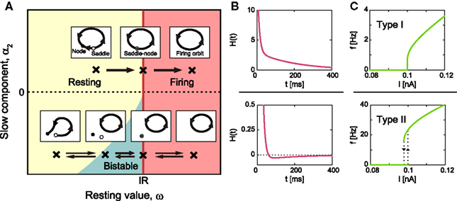
Figure 3. Bifurcation diagram of type I/II excitabilities. (A) Phase diagram in the ω–α₂ plane for arbitrary positive value of α₁ and geometric representation of the model dynamics. The MAT model exhibits saddle-node bifurcation and saddle-node off invariant circle bifurcation in the upper and lower parts of the phase diagram, α₂ ≥ 0 and α₂ < 0, respectively. (B) The corresponding dynamics of adaptive threshold θ(t). (C) The f–I curve. The firing frequency induced by a constant input current increases from zero in the type I phase α₂ ≥ 0, while it exhibits a hysteresis in the type II phase, α₂ < 0. The model parameters for type I: α₁ = 15, α₂ = 3, and ω = 5, and for type II: α₁ = 15, α₂ = −0.05, and ω = 5.

Type I Excitability

In the upper part of the phase diagram of Figure 3A, α₂ ≥ 0, H(t) is a monotonic decreasing function (Figure 3B), and the periodic firing is initiated with the saddle-node bifurcation at IR = ω. Accordingly, the frequency of the oscillation increases continuously from zero, as demonstrated by the continuous f–I curve shown in Figure 3C.

We can analyze the model dynamics by decomposing θ(t)–ω into two variables, and , and drawing the trajectory in the plane of (θ₁, θ₂). Since these variables satisfy differential equations dθ₁/dt = −θ₁/τ₁ and dθ₂/dt = −θ₂/τ₂, we can obtain the differential equation for the trajectory of (θ₁, θ₂) by eliminating time t as

which leads to

where τ₁/τ₂ = 10/200 = 0.05 for the original choice of two timescales, and c is an integration constant.

Given a current I, the MAT model generates a spike if the state (θ₁, θ₂) is in the “firing region,”

and if an absolute refractory period τ_R has expired from the last spike. When the model generates a spike, the state is shifted according to

Figure 4A shows the trajectory for the case of type I excitability. The origin (θ₁, θ₂) = (0, 0) remains as a stable fixed point, or a stable node, if it lies outside the firing region. If the firing region contains (θ₁, θ₂) = (0, 0), the stable node disappears and the repetitive firing, or the limit cycle of oscillation, starts.

FIGURE 4

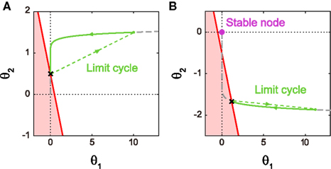
Figure 4. Dynamics of type I and type II firing. Geometric representation of the firing dynamics in the plane of . (A) Type I. (B) Type II. Once the state point meets the boundary of the firing region θ₁ + θ₂ ≤ IR − ω (red solid lines), the state (θ₁, θ₂) is reset to (θ₁ + α₁, θ₂ + α₂) (green dashed lines). The state returns to the initial position along the trajectory (green solid line) given by Eq. 5(gray dashed line). The origin (θ₁, θ₂) = (0, 0) remains as a stable fixed point [a purple closed circle in (B)] if it is outside the firing region. The model parameters for (A): α₁ = 10, α₂ = 1 and IR − ω = 0.5, and for (B): α₁ = 10, α₂ = −0.2 and IR − ω = −0.5.

The period of limit cycle oscillation T is determined by the condition that the shifted state (θ₁ + α₁, θ₂ + α₂) will come back to the initial state (θ₁, θ₂) after the relaxation for a period T. This condition is represented by a set of equations

By eliminating θ₁ and θ₂ from these equations, we obtain the equation that determines the period of oscillation T,

The f–I curve can be obtained by solving this equation for given current I. In a limit of large T, the second term in the left-hand-side dominates, and the equation is approximated as and thus giving

Type II Excitability

In the lower part of ω − α₂ phase diagram of Figure 3A, α₂ < 0, the system exhibits a bifurcation that corresponds to the saddle-node off invariant circle bifurcation for an ordinary differential equation system. In this parameter range, H(t) expresses a dent in response to a single spike (Figure 3B), which makes the system bistable, exhibiting both the resting state and autonomous repetitive firing. The bistability induces a hysteresis in the f–I curve (Figure 3C), with a finite frequency gap induced by the dent in H(t).

The equation for determining the frequency–current relation, Eq. 9, also holds for this case of α₂ < 0. The points of difference from the case of α₂ > 0 are that the trajectory giving a repetitive firing cycle can coexist with the stable fixed point (θ₁, θ₂) = (0, 0) (Figure 4B), and that the limit cycle trajectory disappears before the frequency f = 1/T vanishes.

Burst Firing

For the parameter range of α₁ < 0 and α₂ > 0, Kobayashi et al. (2009) have shown that the MAT model is capable of exhibiting the burst firing. Here, we analyze the bursting in terms of the trajectory of the state (θ₁, θ₂). Figure 5 depicts a closed loop trajectory in which the burst firing is repeated with intermissions of the relaxation periods. In the case of α₁ + α₂ < 0, the occurrence of a spike rather lowers the threshold. If the state (θ₁, θ₂) still remains in the firing region after the absolute refractory period τ_R, the neuron generates another spike. The neuron repeats this resetting until the state escapes from firing region.

FIGURE 5

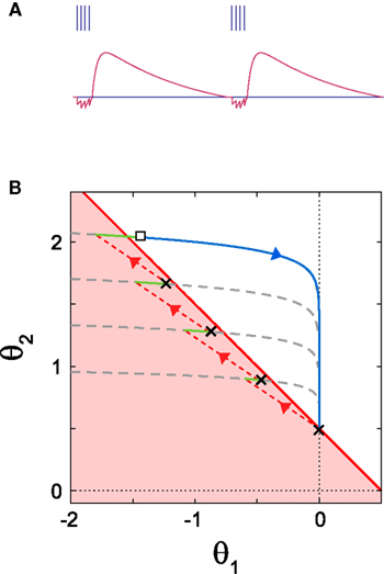
Figure 5. Dynamics of bursting. (A) The time dependence of dynamic threshold θ(t) and the resulting burst firing. (B) Geometric representation of the bursting dynamics in the plane of . Once the state point meets the boundary of the firing region (a red solid line), the system starts to repeat spiking (black crosses), resetting (red dashed lines) and short relaxation for τ_R = 2 ms (green curves). After escaping from the firing region (an open square), the system enters relaxation period (a gray dashed line). The model parameters: α₁ = −0.8, α₂ = 0.5 and IR − ω = 0.5.

The burst firing of N spikes brings the state point (θ₁, θ₂) to

For instance, the burst firing of two spikes starts with the condition of

This condition determines the boundary between the type I and burst firing regions. In the case of IR − ω = 0 as in Figure 2, this is

Unfeasible Region

In the burst firing region, the number of spikes contained in each burst increases by decreasing α₁. By decreasing α₁ further, the system enters an unfeasible region in which the system cannot escape from the firing region. The boundary of this unfeasible region is given by taking the limit N → ∞ in Eq. 11and comparing it with firing condition of Eq. 6. This is given by

In the type II firing region, the firing frequency increases by decreasing α₂. Because the firing frequency should be bounded by 1/τ_R due to the refractory period, the condition of the firing frequency reaching 1/τ_R determines the boundary between the type II and unfeasible region. In the case of IR − ω = 0, the condition becomes

In the limit of τ₂ > τ₁ ≫ τ_R, the boundary between the unfeasible region and the burst firing region (Eq. 14) and the boundary between the unfeasible region and the type II region (Eq. 15) asymptotically approach to a single straight line, α₂ = −(τ₁/τ₂)α₁.

Augmentation of the MAT Model with Voltage Dependency

We have shown above that the MAT model is capable of exhibiting basic dynamic characteristics, such as type I/II excitability and burst firing, but we show in the next section that the original model is not sufficiently flexible to exhibit a richer variety of responses of biological neurons to transient input currents, summarized as Izhikevich’s table (Izhikevich, 2004).

The reason that the original MAT model cannot represent a variety of firing responses to dynamic input current is that the adaptive threshold does not depend on the present state of voltage. Therefore, we suggest extending the adaptive threshold dynamics of the MAT model by adding a term representing the voltage dependency of the form

where β is a parameter for controlling the voltage dependency, and K(s) is an α-function kernel of timescale τ_V,

This dependency of the spiking threshold on the derivative of membrane voltage was actually observed in biological neurons (Azouz and Gray, 2000) and is considered to have resulted from activation/inactivation dynamics of voltage-gated sodium channels (Naundorf et al., 2006; Platkiewicz and Brette, 2011), or the backpropagation of axonal spike to the soma (Yu et al., 2008). The timescale τ_V of the influence of dV/dt dependency is estimated as a few ms (Azouz and Gray, 2000); we fixed this time constant at 5 ms. Thus, the tunable parameter for this voltage dependency is only the coefficient β.

Due to the linear kernel integration with the alpha function kernel, the numerical integration of this model can be expedited by rewriting the evolution equation into a set of differential equations. By rewriting the evolution equation in this way, it is possible to implement the algorithm of exact subthreshold integration (Morrison et al., 2007; Plesser and Diesmann, 2009), which we discuss in the Section “Appendix.”

Variety of Firing Responses Realized by the Original and Augmented MAT Models

In this section, we consider numerous transient input current types, including step currents, ramp currents, and a set of short current pulses, and we examine whether the original and augmented MAT models are capable of handling the 20 qualitative firing responses defined by Izhikevich (2004).

Original MAT Model

We found that the original MAT model is capable of reproducing 9 of the 20 basic firing responses, as shown in Figures 6A–I. More specifically, the model produces basic tonic spiking in response to a step current (Figure 6A), frequency adaptation (Figure 6B), integrator (Figure 6C), class 1 (type I) excitability (Figure 6D), class 2 (type II) excitability (Figure 6E), and bistability (Figure 6F). The terms class 1/2 are used in the original paper by Hodgkin (1948), whereas they are also referred to as type I/II in terms of the connection to bifurcations (Rinzel and Ermentrout, 1989). For the type II parameter region shown in Figure 2, the threshold may exhibit a dent after a spike, which can be interpreted as depolarizing after-potential that helps the occurrence of a successive spike (Figure 6G). In the region of bursting shown in Figure 2, the MAT model exhibits tonic bursting to a step current injection (Figure 6H). Given parameters near the boundary between the bursting and type I regions of Figure 2, the model shows burst firing only at the onset of a step current injection, and then starts tonic spiking (Figure 6I).

FIGURE 6

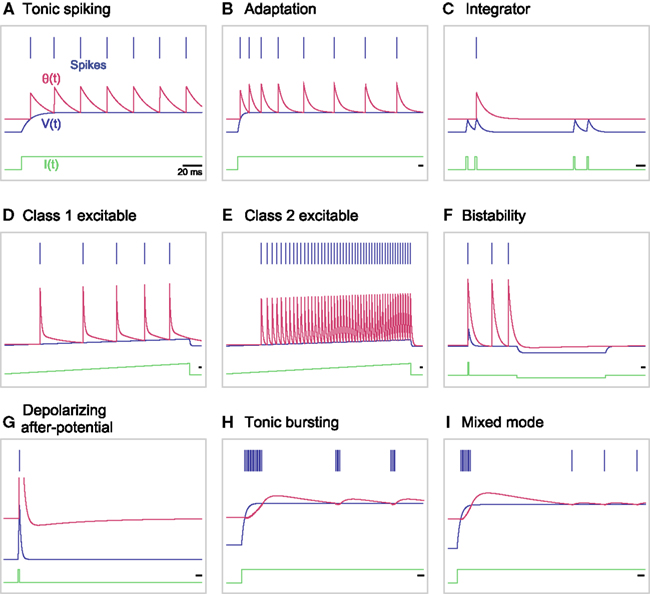
Figure 6. A variety of firing responses manifested by the original MAT model. (A) basic tonic spiking; (B) frequency adaptation; (C) integrator; (D) class 1 excitability; (E) class 2 excitability; (F) bistability; (G) depolarizing after-potential; (H) tonic bursting; and (I) mixed mode. The blue bars indicate the generated spikes. The red, blue and green traces represent the adaptive threshold, the model potential, and the input current, respectively.

Augmented MAT Model

The original MAT model cannot complete the entire set of firing responses, because the dynamics of the adaptive threshold is only dependent on past spikes and does not depend on the present state of the membrane voltage. To enable the MAT model to respond variably to time-dependent input current, we have augmented the adaptive threshold dynamics of the model by adding a term representing the voltage dependency (using Eqs 16 and 17 above). Figures 7A–K shows 11 firing patterns that are successfully realized by our augmented MAT model; each firing pattern is listed below. Due to the sensitivity to dV/dt, the augmented model can exhibit phasic spiking or bursting; more specifically, the neuron emits a spike or a burst of spikes only at the onset of a step current injection (Figures 7A,B), exhibits delayed response to short pluses (Figure 7C), shows rebound spiking or bursting (Figures 7D,E), and exhibits threshold variability (Figure 7F).

FIGURE 7

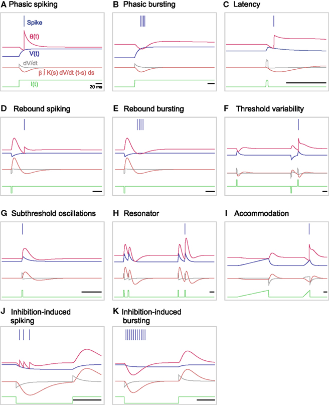
Figure 7. A variety of firing responses manifested by the augmented MAT model. (A) phasic spiking; (B) phasic bursting; (C) latency; (D) rebound spiking; (E) rebound bursting; (F) threshold variability; (G) subthreshold oscillations; (H) resonator; (I) accommodation; (J) inhibition-induced spiking; and (K) inhibition-induced bursting. Note that this entire set of firing responses follows definitions in Izhikevich (2004). The blue bars indicate the generated spikes. The red, blue, and green traces represent the adaptive threshold, the model potential, and the input current, respectively. The gray and orange traces are the value of dV/dt and the voltage dependent term, respectively.

Furthermore, our augmented MAT model can mimic subthreshold oscillation in which the dynamic threshold follows the increases and decreases in voltage (Figure 7G). According to the transient oscillation mimicked by the dynamic threshold, the model may behave as a resonator, firing in response to a pair of input pulses with a particular interval (Figure 7H); for detailed conditions of such a resonator, please see the Section “Appendix.” The dV/dt dependency induces an effect of accommodation (Figure 7I). With our augmented model, the neuron is also able to elicit spikes or bursts in response to inhibitory input, an approach called inhibition-induced spiking or bursting (Figures 7J,K).

The model parameters and input conditions that were used for reproducing these responses are summarized in Table 1. The locations of these model parameters in the space of α₁, α₂, and β are depicted in Figure 8. Some of the firing responses, such as class 1 vs class 2, or integrator vs resonator are mutually exclusive by definition. However, there are cases in which multiple firing response types can be realized with the same set of model parameters solely by changing the input conditions. Such degeneracy occurs, for instance, between phasic spiking, latency, threshold variability, accommodation, and rebound spiking, or between phasic bursting, rebound bursting, and tonic bursting.

TABLE 1

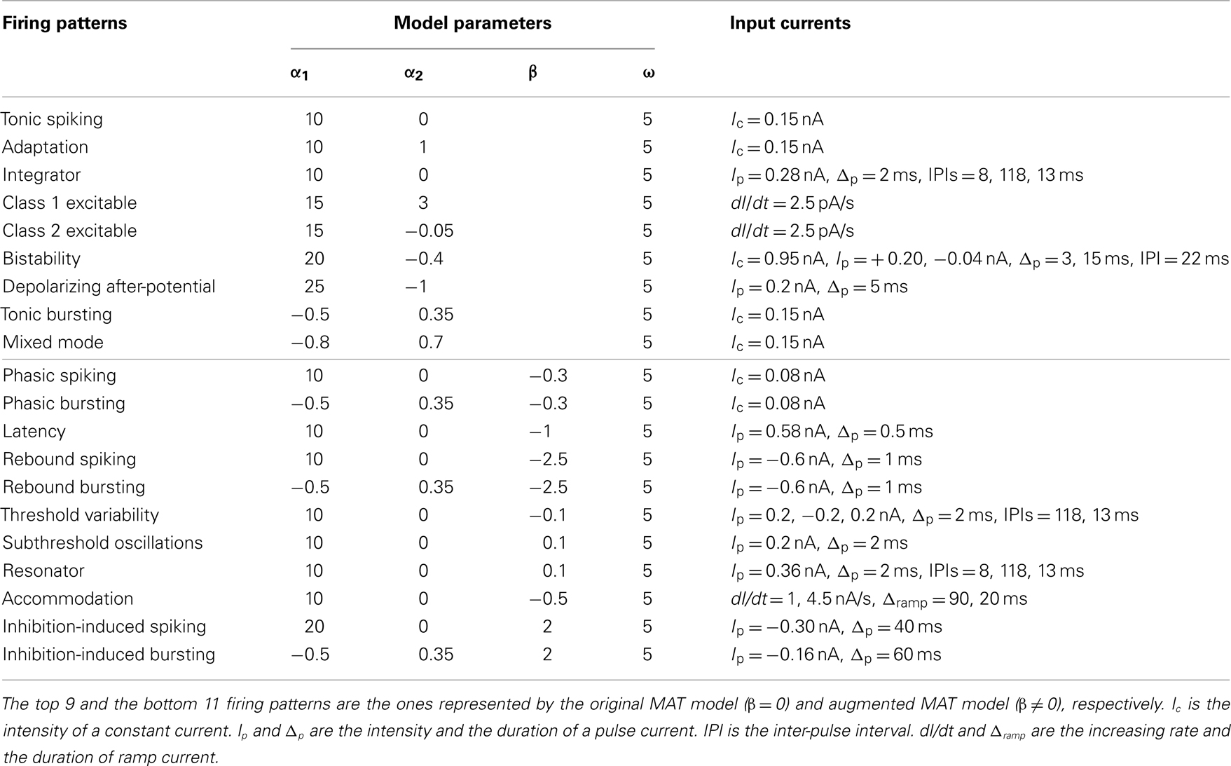
Table 1. Model parameters and input currents used for reproducing firing patterns in Figures 6 and 7.

FIGURE 8

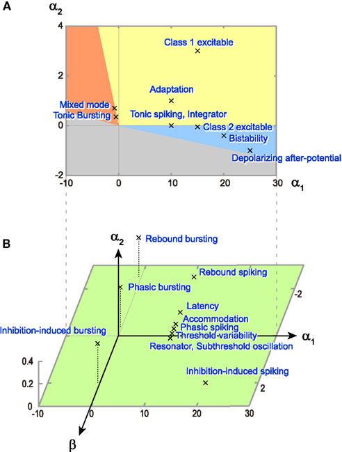
Figure 8. Distribution of model parameters that realized a variety of firing patterns. (A) Parameter values (α₁, α₂) of the original MAT model, which are used to reproduce nine firing patterns in Figure 6. The colors of the firing type regions are the same as Figure 2. (B) Parameter values (α₁, α₂, β) of the augmented MAT model, which are used to reproduce 11 firing patterns in Figure 7. The numerical values of the respective model parameters are summarized in Table 1.

Reproducing the Quantitative Features of Biological Neuronal Firing

It was reported that the original MAT model can reproduce the qualitative features of four representative firing types, FS, RS, IB, and CH neurons (Kobayashi et al., 2009). However, the model does not necessarily account for them quantitatively. To be precise, the original MAT model is capable of reproducing FS, RS, and CH firing, but the model should be augmented with the voltage dependent term in order to reproduce IB firing in a range of biologically acceptable timescales. Here we demonstrate the typical parameter setting of the model in reproducing the biological neuronal firing patterns.

FS neurons

They fire high-frequency tonic spikes with little or no frequency adaptation. The original MAT model (β = 0) is capable of reproducing the tonic firing of 200 Hz in response to a rectangular current of 0.6 nA (McCormick et al., 1985) with the model parameters of α₁ = 10, α₂ = 0, and ω = 15. Note that even the multiple timescales are not necessarily needed for this case, and the simple LIF model is enough to reproduce the phenomena.

RS neurons

They fire tonic spikes with adapting frequency in response to rectangular current, and have class 1 excitability. This can also be represented by the original MAT model. For instance, the model is capable of reproducing the situation in which the neuron is injected a rectangular current of 0.6 nA and exhibits initial firing frequency of 120 Hz as defined from the first interspike interval and adapts the firing frequency to 30 Hz (McCormick et al., 1985) with the parameters of α₁ = 20, α₂ = 2, and ω = 20. Having two timescales is necessary for reproducing the frequency adaptation.

CH neurons

They fire high-frequency bursts of a few (<5) spikes with relatively constant inter-burst interval of 15–50 ms (Gray and McCormick, 1996). When reproducing CH firing by the original MAT model, the inter-burst interval in the tonic bursting is determined by the relaxation of the slow component. The MAT model can reproduce tonic bursting of inter-burst frequency of 20 Hz and intra-burst frequency of 500 Hz in response to a rectangular current of 0.6 nA, respectively (Nowak et al., 2003), with the parameters of α₁ = −2.5, α₂ = 2, and ω = 28.

IB neurons

They generate a burst of three to five spikes at the beginning of a strong depolarizing pulse of current, and then switch to tonic spiking. Intra-burst frequency is low compared to CH neurons (Gray and McCormick, 1996; Nowak et al., 2003). Though we demonstrated that the original MAT model is capable of representing the mixed mode (Figure 6I), the intra-burst frequency in this case becomes 1/τ_R = 500 Hz, which is outside the biologically plausible range (≤350 Hz; Nowak et al., 2003). Thus the MAT model has to be augmented with the voltage dependent term to generate the depolarizing wave evoked by the current injection (McCormick et al., 1985). The augmented MAT model can reproduce the IB firing with frequencies of the burst and tonic modes of 300 Hz and 30 Hz, respectively (Nowak et al., 2003) with the model parameters of α₁ = 9, α₂ = 0.3, β = −0.3, and ω = 28.

Other types of neurons

In addition to those four representative firing types, there are more abundant firing responses (Kawaguchi, 1995; Kawaguchi and Kondo, 2002; Markram et al., 2004; Izhikevich, 2007; Ascoli et al., 2008). In the following, we show the parameter values with which the augmented MAT model is capable of reproducing them.

The low-threshold spiking (LTS) neurons respond in a manner identical to RS neurons to a prolonged suprarheobasic current injection at depolarized potentials, and respond to current injections just greater than rheobase with a transient bursting of two or more spikes with short (<20 ms) ISIs at hyperpolarized potentials. The augmented MAT model is capable of reproducing the response with the parameters of α₁ = 10, α₂ = 1, β = −0.2, and ω = 25.

Phasic spiking or phasic bursting was observed from inhibitory interneurons in the rat frontal cortex (Kawaguchi and Kondo, 2002). Our augmented MAT model can reproduce phasic spiking and bursting in response to a rectangular current of 0.6 nA with the parameters of α₁ = 20, α₂ = 1, β = −0.3, and ω = 35 and α₁ = −2.2, α₂ = 2, β = −0.3, and ω = 35, respectively. By increasing current intensity, the model with these sets of parameters can generate tonic spiking or bursting.

The thalamocortical (TC) neurons are known to possess firing regimes of tonic spiking and rebound bursting as in LTS neurons, but their adaptation is smaller than LTS neurons (Llinás and Jahnsen, 1982; Destexhe and Sejnowski, 2001). For instance, our augmented MAT model can reproduce such a response with the parameters of α₁ = 10, α₂ = 0, β = −0.2, and ω = 25. Although inhibition-induced spiking or bursting (Figures 7J,K) is a specific feature of TC neurons (Izhikevich, 2003), we have not found a set of model parameters with which the model can realize both the inhibition-induced firing and rebound bursting (see Table 1).

In contrast to TC neurons, a certain type of thalamic interneuron does not have a burst regime, though they can fire rebound spikes (Pape and McCormick, 1995). Except for rebound spiking, this type of thalamic interneuron can fire high-frequency tonic spikes without pronounced frequency adaptation, like FS neurons. Our augmented MAT model can reproduce such a response with the parameters of α₁ = 5, α₂ = 0, β = −0.1, and ω = 25. Note that there is a different type of interneuron in thalamus that generates robust action potential bursts after an inhibitory input (Bal and McCormick, 1993), which our model cannot reproduce.

Reproducing and Predicting Biological Neuronal Responses to Fluctuating Currents

In the preceding section, we showed that our augmented MAT model is capable of reproducing rebound spiking and a variety of responses induced by threshold variability. As the number of parameters increases, in general, it is likely to become less capable of accommodating the numerical data. In this section, we examine whether the augmented MAT model still has the ability to predict biological spike times through the augmentation of voltage dependency.

In our examination, we use publicly available data from the International Competition on Quantitative Single-Neuron Modeling 2009 [Gerstner and Naud, 2009; International Neuroinformatics Coordinating Facility (INCF), 2009] in which the original MAT model demonstrated the ability to predict spikes, and therefore won first place in the competition. The publicly available data consisted of in vivo-like fluctuating input current and the voltage responses of 13 trials recorded from a L5 pyramidal neuron.

We adjusted the model parameters to match the data of 10 randomly selected trials, and then validated the ability of our augmented MAT model to predict the remaining 3 trials. We evaluated average predictive ability by repeating this random sampling process 100 times. The adaptive capability of the model in predicting spike times was assessed using a coefficient measuring the fraction of spikes that coincided in 4 ms between a model spike train and a real biological spike train. Among various measures (including Victor and Purpura, 1996; Tsubo et al., 2004), we adopted coincidence factor γ as introduced in the competition (Jolivet et al., 2004, 2006, 2008; Kobayashi and Shinomoto, 2007).

Based on the above procedure, the predictive performance of the original MAT model was 0.77, whereas the augmented MAT model was 0.84, as summarized in Table 2. We also compared the performance of these models using the different coincidence windows ranging from 2 to 10 ms, and confirmed the consistent superiority of the augmented MAT model to the original model. Clearly, the augmentation does not cause predictive ability to deteriorate, but rather improves it. Figure 9 demonstrates the spike prediction of the original and augmented MAT models. From the sampling shown in the figure, both models attain similar predictive performance in the stationary period of high input current (17.5–18 and 20–21 s); however, the augmented MAT model is more proficient than the original model in predicting spikes in the period of weak input current (18.8–19.5 and 21–21.5 s) by responding to small peaks of model potential.

TABLE 2

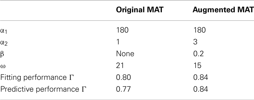
Table 2. Optimized parameters of the original and augmented MAT models fitted to the biological data and their fitting and predictive performances.

FIGURE 9

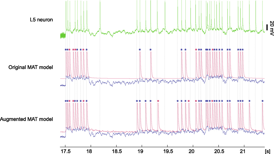
Figure 9. Model prediction for spiking response of a L5 pyramidal neuron to fluctuating current. The top column is a voltage trace of the experimental data obtained from an L5 neuron (data #9, Challenge A in the International Competition on Quantitative Single-Neuron Modeling 2009). The middle and bottom columns are spike times predicted by the original and augmented MAT models. The model potential and adaptive threshold are depicted in blue and red, respectively. Spikes are asterisked in blue or red, according to whether they coincided with experimental data within 4 ms. Dotted lines represent experimental spike times.

Discussion

Numerical simulations of realistic neuronal microcircuitry have been primarily based on the Hodgkin–Huxley model (Traub et al., 2005; Markram, 2006) or the LIF model (Diesmann et al., 1999; Gewaltig and Diesmann, 2007). As noted by Izhikevich (2004), these models typically have a conflict between biological reality and computational efficiency. The non-linear model proposed by Izhikevich (2004) and the linear model proposed by Mihalas and Niebur (2009) would be exceptional models that evade such a conflict.

The original MAT model possesses the strongest ability to reproduce and predict precise spike times, but is unable to reproduce the full variety of firing responses demonstrated by Izhikevich (2004). In this paper, we have proposed a revision of the MAT model in which the full variety of firing responses given by Izhikevich (2004) is successfully reproduced. We thoroughly analyzed the dynamic characteristics of the original model and augmented model, the latter including a voltage dependency term. We also showed that our augmented model does not decrease its predictive ability in comparison to the original MAT model, but rather improves quantitative predictive ability.

Voltage Dependency of Spiking Threshold

The variability of spike threshold has been observed in numerous physiological experiments (Azouz and Gray, 2000; Ferragamo and Oertel, 2002; de Polavieja et al., 2005; Wilent and Contreras, 2005; Naundorf et al., 2006), and Hodgkin–Huxley-style models that can reproduce the threshold variability were proposed (Azouz and Gray, 2003; Naundorf et al., 2006; McCormick et al., 2007; Colwell and Brenner, 2009). More recently, Platkiewicz and Brette (2010) deduced a threshold equation that explained the manner in which the spike threshold varies with the membrane potential, depending on ionic channel properties.

There are also simplified models that introduce voltage dependency into the threshold in the LIF model (originally in Hill, 1936). Dodla et al. (2006) proposed a model that explains post-inhibitory facilitation by introducing the threshold depending on the instantaneous value of voltage with mono-exponential decay. Mihalas and Niebur (2009) adopted this form of the voltage dependency and demonstrated that the model was able to reproduce a wide variety of firing responses to various transient current inputs. Experimental research by Azouz and Gray (2000) indicated that the spike threshold related inversely with the time derivative of membrane potential. We incorporated this relationship straightforwardly into the threshold dynamics of the original MAT model while preserving its linearity, succeeding in reproducing the variety of firing patterns in Izhikevich’s table.

It would be worth noticing that the origin of the threshold variability is still in controversy. A recent study suggested that the threshold variability seen in experiments could be an artifact (Yu et al., 2008); because spikes are initiated not in the soma but in the axon initial segment, the threshold variability of the firing seen in intracellular recordings can be largely attributed by its backpropagation to the soma. Contrariwise, Platkiewicz and Brette (2011) asserted that the backpropagation cannot be the dominant cause of the threshold variability; they suggested that sodium channel inactivation is a strong candidate for the mechanism responsible for the threshold variability.

Comparison with Other Simplistic Spike Neuron Models

To end our discussion, we compare our augmented MAT model with other eminent simplistic spike neuron models. The Izhikevich model is a concise non-linear model that has succeeded in demonstrating a diversity of firing responses by controlling only a few parameters. The adaptive exponential integrate-and-fire (AdEx) model (Brette and Gerstner, 2005), which combines features of the exponential integrate-and-fire model (Fourcaud-Trocmé et al., 2003) with the two-variable Izhikevich model, is also able to account for a large variety of firing patterns (Naud et al., 2008; Touboul and Brette, 2009). In comparison with these models, a key strength of our augmented MAT model is its linearity, which makes it straightforward to efficiently simulate a large network of spiking neurons using the method of exact subthreshold integration (Morrison et al., 2007; Plesser and Diesmann, 2009).

The Mihalas–Niebur model is a tractable linear model that describes burst firing in terms of after-potentials in a more realistic manner than that of the MAT model, which mechanistically repeats the regular firing given by a prefixed absolute refractory period τ_R = 2 ms. The Mihalas–Niebur model is capable of demonstrating most firing responses, except for resonate firing in Izhikevich’s table. The reason that the augmented MAT model is able to reproduce resonate firing is that the alpha function kernel naturally induces a delay in the voltage dependency.

The original MAT model can be regarded as a subtype of the SRM, which may describe arbitrary dependency of neuronal excitability on previous spiking history within a linear framework (Gerstner and Kistler, 2002). With an augmentation of voltage dependency in the threshold equation, the augmented MAT model can be considered as one expression of the Mihalas–Niebur model. Indeed, the SRM or the Mihalas–Niebur model has a great ability to adapt to experimental data due to its large degree of freedom. However, such a high adaptability of the model sometimes causes over-fitting to the finite data, and as a result, reduces its predictive performance. Thus our model, which has a restricted number of free parameters, can be more competent in simulating neuronal circuitry faithfully, given practically available data.

Conflict of Interest Statement

The authors declare that the research was conducted in the absence of any commercial or financial relationships that could be construed as a potential conflict of interest.

Acknowledgments

We are grateful to R. Kobayashi for insightful comments, and two reviewers for their constructive advices that helped to drastically improve the manuscript. We greatly acknowledge R. Naud and W. Gerstner, who have made their data publicly available. This study was supported in part by Grants-in-Aid for Scientific Research to Shigeru Shinomoto from MEXT Japan (20300083, 23115510) and a Grant-in-Aid for the Global COE Program “The Next Generation of Physics, Spun from Universality and Emergence” from the MEXT of Japan. Hideaki Kim is supported by a Grant-in-Aid for JSPS Fellows.

References

Ascoli, G. A., Alonso-Nanclares, L., Anderson, S. A., Barrionuevo, G., Benavides-Piccione, R., Burkhalter, A., Buzsáki, G., Cauli, B., Defelipe, J., Fairén, A., Feldmeyer, D., Fishell, G., Fregnac, Y., Freund, T. F., Gardner, D., Gardner, E. P., Goldberg, J. H., Helmstaedter, M., Hestrin, S., Karube, F., Kisvárday, Z. F., Lambolez, B., Lewis, D. A., Marin, O., Markram, H., Muñoz, A., Packer, A., Petersen, C. C., Rockland, K. S., Rossier, J., Rudy, B., Somogyi, P., Staiger, J. F., Tamas, G., Thomson, A. M., Toledo-Rodriguez, M., Wang, Y., West, D. C., and Yuste, R. (2008). Petilla terminology, nomenclature of features of GABAergic interneurons of the cerebral cortex. Nat. Rev. Neurosci. 9, 557–568.

Pubmed Abstract | Pubmed Full Text | CrossRef Full Text

Azouz, R., and Gray, C. M. (2000). Dynamic spike threshold reveals a mechanism for synaptic coincidence detection in cortical neurons in vivo. Proc. Natl. Acad. Sci. U.S.A. 97, 8110–8115.

Pubmed Abstract | Pubmed Full Text | CrossRef Full Text

Azouz, R., and Gray, C. M. (2003). Adaptive coincidence detection and dynamic gain control in visual cortical neurons in vivo. Neuron 37, 513–523.

Pubmed Abstract | Pubmed Full Text | CrossRef Full Text

Badel, L., Lefort, S., Brette, R., Petersen, C. C. H., Gerstner, W., and Richardson, M. J. E. (2008). Dynamic I-V curves are reliable predictors of naturalistic pyramidal-neuron voltage traces. J. Neurophysiol. 99, 656–666.

Pubmed Abstract | Pubmed Full Text | CrossRef Full Text

Bal, T., and McCormick, D. A. (1993). Mechanisms of oscillatory activity in guinea-pig nucleus reticularis thalami in vitro: a mammalian pacemaker. J. Physiol. 468, 669–691.

Pubmed Abstract | Pubmed Full Text

Brandman, R., and Nelson, M. E. (2002). A simple model of long-term spike train regularization. Neural Comput. 14, 1575–1597.

Pubmed Abstract | Pubmed Full Text | CrossRef Full Text

Brette, R., and Gerstner, W. (2005). Adaptive exponential integrate-and-fire model as an effective description of neuronal activity. J. Neurophysiol. 94, 3637–3642.

Pubmed Abstract | Pubmed Full Text | CrossRef Full Text

Brette, R., Rudolph, M., Carnevale, T., Hines, M., Beeman, D., Bower, J. M., Diesmann, M., Morrison, A., Goodman, P. H., Harris, F. C. Jr., Zirpe, M., Natschläger, T., Pecevski, D., Ermentrout, B., Djurfeldt, M., Lansner, A., Rochel, O., Vieville, T., Muller, E., Davison, A. P., El Boustani, S., and Destexhe, A. (2007). Simulation of networks of spiking neurons: a review of tools and strategies. J. Comput. Neurosci. 23, 349–398.

Pubmed Abstract | Pubmed Full Text | CrossRef Full Text

Burkitt, A. N. (2006). A review of the integrate-and-fire neuron model: I. Homogeneous synaptic input. Biol. Cybern. 95, 1–19.

Pubmed Abstract | Pubmed Full Text | CrossRef Full Text

Chacron, M. J., Pakdaman, K., and Longtin, A. (2003). Interspike interval correlations, memory, adaptation, and refractoriness in a leaky integrate-and-fire model with threshold fatigue. Neural Comput. 15, 253–278.

Pubmed Abstract | Pubmed Full Text | CrossRef Full Text

Colwell, L. J., and Brenner, M. P. (2009). Action potential initiation in the Hodgkin–Huxley model. PLoS Comput. Biol. 5, e1000265. doi: 10.1371/journal.pcbi.1000265

Pubmed Abstract | Pubmed Full Text | CrossRef Full Text

de Polavieja, G. G., Harsch, A., Kleppe, I., Robinson, H. P. C., and Juusola, M. (2005). Stimulus history reliably shapes action potential waveforms of cortical neurons. J. Neurosci. 25, 5657–5665.

Pubmed Abstract | Pubmed Full Text | CrossRef Full Text

Destexhe, A., and Sejnowski, T. J. (2001). Thalamocortical Assemblies. New York: Oxford University Press.

Diesmann, M., Gewaltig, M.-O., and Aertsen, A. (1999). Stable propagation of synchronous spiking in cortical neural networks. Nature 402, 529–533.

Pubmed Abstract | Pubmed Full Text | CrossRef Full Text

Dodla, R., Svirskis, G., and Rinzel, J. (2006). Well-timed, brief inhibition can promote spiking: postinhibitory facilitation. J. Neurophysiol. 95, 2664–2677.

Pubmed Abstract | Pubmed Full Text | CrossRef Full Text

Ferragamo, M. J., and Oertel, D. (2002). Octopus cells of the mammalian ventral cochlear nucleus sense the rate of depolarization. J. Neurophysiol. 87, 2262–2270.

Pubmed Abstract | Pubmed Full Text

Fourcaud-Trocmé, N., Hansel, D., van Vreeswijk, C., and Brunel, N. (2003). How spike generation mechanisms determine the neuronal response to fluctuating inputs. J. Neurosci. 23, 11628–11640.

Pubmed Abstract | Pubmed Full Text

Geisler, C. D., and Goldberg, J. M. (1966). A stochastic model of the repetitive activity of neurons. Biophys. J. 6, 53–69.

Pubmed Abstract | Pubmed Full Text | CrossRef Full Text

Gerstner, W. (1995). Time structure of the activity in neural network models. Phys. Rev. E 51, 738–758.

CrossRef Full Text

Gerstner, W., and Kistler, W. M. (2002). Spiking Neuron Models: Single Neurons, Populations, Plasticity. Cambridge: Cambridge University Press.

Gerstner, W., and Naud, R. (2009). How good are neuron models? Science 326, 379–380.

Pubmed Abstract | Pubmed Full Text | CrossRef Full Text

Gerstner, W., and van Hemmen, J. L. (1992). Associative memory in a network of “spiking” neurons. Network 3, 139–164.

CrossRef Full Text

Gewaltig, M.-O., and Diesmann, M. (2007). NEST. Scholarpedia 2, 1430.

CrossRef Full Text

Gray, C. M., and McCormick, D. A. (1996). Chattering cells: superficial pyramidal neurons contributing to the generation of synchronous oscillations in the visual cortex. Science 274, 109–113.

Pubmed Abstract | Pubmed Full Text | CrossRef Full Text

Hill, A. V. (1936). Excitation and accommodation in nerve. Proc. R. Soc. Lond. B Biol. Sci. 119, 305–355.

CrossRef Full Text

Hille, B. (2001). Ion Channels of Excitable Membranes. Sunderland, MA: Sinauer Associates.

Hodgkin, A. L. (1948). The local electric changes associated with repetitive action in a non-medullated axon. J. Physiol. 107, 165–181.

Pubmed Abstract | Pubmed Full Text

Hodgkin, A. L., and Huxley, A. F. (1952). A quantitative description of membrane current and its application to conduction and excitation in nerve. J. Physiol. 117, 500–544.

Pubmed Abstract | Pubmed Full Text

Hoppensteadt, F. C., and Izhikevich, E. M. (1997). Weakly Connected Neural Networks. New York: Springer-Verlag.

International Neuroinformatics Coordinating Facility (INCF). (2009). Quantitative Single-Neuron Modeling. Available at: http://www.incf.org/Events/competitions/spike-time-prediction/2009

Izhikevich, E. M. (2001). Resonate-and-fire neurons. Neural Netw. 14, 883–894.

Pubmed Abstract | Pubmed Full Text | CrossRef Full Text

Izhikevich, E. M. (2003). Simple model of spiking neurons. IEEE Trans. Neural Netw. 14, 1569–1572.

Pubmed Abstract | Pubmed Full Text | CrossRef Full Text

Izhikevich, E. M. (2004). Which model to use for cortical spiking neurons? IEEE Trans. Neural Netw. 15, 1063–1070.

Pubmed Abstract | Pubmed Full Text | CrossRef Full Text

Izhikevich, E. M. (2007). Dynamical Systems in Neuroscience: The Geometry of Excitability and Bursting. Cambridge: MIT Press.

Izhikevich, E. M., and Edelman, G. M. (2008). Large-scale model of mammalian thalamocortical systems. Proc. Natl. Acad. Sci. U.S.A. 105, 3593–3598.

Pubmed Abstract | Pubmed Full Text | CrossRef Full Text

Jolivet, R., Lewis, T. J., and Gerstner, W. (2004). Generalized integrate-and-fire models of neuronal activity approximate spike trains of a detailed model to a high degree of accuracy. J. Neurophysiol. 92, 959–976.

Pubmed Abstract | Pubmed Full Text | CrossRef Full Text

Jolivet, R., Rauch, A., Lüscher, H.-R., and Gerstner, W. (2006). Predicting spike timing of neocortical pyramidal neurons by simple threshold models. J. Comput. Neurosci. 21, 35–49.

Pubmed Abstract | Pubmed Full Text | CrossRef Full Text

Jolivet, R., Schürmann, F., Berger, T. K., Naud, R., Gerstner, W., and Roth, A. (2008). The quantitative single-neuron modeling competition. Biol. Cybern. 99, 417–426.

Pubmed Abstract | Pubmed Full Text | CrossRef Full Text

Kawaguchi, Y. (1995). Physiological subgroups of nonpyramidal cells with specific morphological characteristics in layer II/III of rat frontal cortex. J. Neurosci. 15, 2638–2655.

Pubmed Abstract | Pubmed Full Text

Kawaguchi, Y., and Kondo, S. (2002). Parvalbumin, somatostatin and cholecystokinin as chemical markers for specific GABAergic interneuron types in the rat frontal cortex. J. Neurocytol. 31, 277–287.

Pubmed Abstract | Pubmed Full Text | CrossRef Full Text

Kistler, W., Gerstner, W., and van Hemmen, J. L. (1997). Reduction of the Hodgkin-Huxley equations to a single variable threshold model. Neural Comput. 9, 1015–1045.

CrossRef Full Text

Kobayashi, R., and Shinomoto, S. (2007). State space method for predicting the spike times of a neuron. Phys. Rev. E 75, 011925.

CrossRef Full Text

Kobayashi, R., Tsubo, Y., and Shinomoto, S. (2009). Made-to-order spiking neuron model equipped with a multi-timescale adaptive threshold. Front. Comput. Neurosci. 3:9. doi: 10.3389/neuro.10.009.2009

Pubmed Abstract | Pubmed Full Text | CrossRef Full Text

Koch, C. (1999). Biophysics of Computation: Information Processing in Single Neurons. Oxford: Oxford University Press.

Llinás, R. R. (1988). The intrinsic electrophysiological properties of mammalian neurons: insights into central nervous system function. Science 242, 1654–1664.

Pubmed Abstract | Pubmed Full Text | CrossRef Full Text

Llinás, R. R., and Jahnsen, H. (1982). Electrophysiology of mammalian thalamic neurones in vitro. Nature 297, 406–408.

Pubmed Abstract | Pubmed Full Text | CrossRef Full Text

Mainen, Z. F., and Sejnowski, T. J. (1995). Reliability of spike timing in neocortical neurons. Science 268, 1503–1506.

Pubmed Abstract | Pubmed Full Text | CrossRef Full Text

Markram, H. (2006). The blue brain project. Nat. Rev. Neurosci. 7, 153–160.

Pubmed Abstract | Pubmed Full Text | CrossRef Full Text

Markram, H., Toledo-Rodriguez, M., Wang, Y., Gupta, A., Silberberg, G., and Wu, C. (2004). Interneurons of the neocortical inhibitory system. Nat. Rev. Neurosci. 5, 793–807.

Pubmed Abstract | Pubmed Full Text | CrossRef Full Text

McCormick, D. A., Connors, B. W., Lighthall, J. W., and Prince, D. A. (1985). Comparative electrophysiology of pyramidal and sparsely spiny stellate neurons of the neocortex. J. Neurosci. 54, 782–806.

McCormick, D. A., Shu, Y., and Yu, Y. (2007). Neurophysiology: Hodgkin and Huxley model–still standing? Nature 445, E1–E2; discussion E2–E3.

Pubmed Abstract | Pubmed Full Text | CrossRef Full Text

McIntyre, C. C., Grill, W. M., Sherman, D. L., and Thakor, N. V. (2004). Cellular effects of deep brain stimulation: model-based analysis of activation and inhibition. J. Neurophysiol. 91, 1457–1469.

Pubmed Abstract | Pubmed Full Text | CrossRef Full Text

Mihalas, S., and Niebur, E. (2009). A generalized linear integrate-and-fire neural model produces diverse spiking behaviors. Neural Comput. 21, 704–718.

Pubmed Abstract | Pubmed Full Text | CrossRef Full Text

Morrison, A., Straube, S., Plesser, H. E., and Diesmann, M. (2007). Exact subthreshold integration with continuous spike times in discrete-time neural network simulations. Neural Comput. 19, 47–79.

Pubmed Abstract | Pubmed Full Text | CrossRef Full Text

Naud, R., Marcille, N., Clopath, C., and Gerstner, W. (2008). Firing patterns in the adaptive exponential integrate-and-fire model. Biol. Cybern. 99, 335–347.

Pubmed Abstract | Pubmed Full Text | CrossRef Full Text

Naundorf, B., Wolf, F., and Volgushev, M. (2006). Unique features of action potential initiation in cortical neurons. Nature 440, 1060–1063.

Pubmed Abstract | Pubmed Full Text | CrossRef Full Text

Nowak, L. G., Azouz, R., Sanchez-Vives, M. V., Gray, C. M., and McCormick, D. A. (2003). Electrophysiological classes of cat primary visual cortical neurons in vivo as revealed by quantitative analyses. J. Neurophysiol. 89, 1541–1566.

Pubmed Abstract | Pubmed Full Text | CrossRef Full Text

Pape, H. C., and McCormick, D. A. (1995). Electrophysiological and pharmacological properties of interneurons in the cat dorsal lateral geniculate nucleus. Neuroscience 68, 1105–1125.

Pubmed Abstract | Pubmed Full Text | CrossRef Full Text

Platkiewicz, J., and Brette, R. (2010). A threshold equation for action potential initiation. PLoS Comput. Biol. 6, e1000850. doi: 10.1371/journal.pcbi.1000850

Pubmed Abstract | Pubmed Full Text | CrossRef Full Text

Platkiewicz, J., and Brette, R. (2011). Impact of fast sodium channel inactivation on spike threshold dynamics and synaptic integration. PLoS Comput. Biol. 7, e1001129. doi: 10.1371/journal.pcbi.1001129

Pubmed Abstract | Pubmed Full Text | CrossRef Full Text

Plesser, H. E., and Diesmann, M. (2009). Simplicity and efficiency of integrate-and-fire neuron models. Neural Comput. 21, 353–359.

Pubmed Abstract | Pubmed Full Text | CrossRef Full Text

Rinzel, J., and Ermentrout, G. B. (1989). “Analysis of neural excitability and oscillations,” in Methods in Neuronal Modeling, eds C. Koch and I. Segev (Cambridge, MA: MIT Press), 251–291.

Rossant, C., Goodman, D. F. M., Fontaine, B., Platkiewicz, J., Magnusson, A. K., and Brette, R. (2011). Fitting neuron models to spike trains. Front. Neurosci. 5:9. doi: 10.3389/fnins.2011.00009

Pubmed Abstract | Pubmed Full Text | CrossRef Full Text

Rotter, S., and Diesmann, M. (1999). Exact digital simulation of time-invariant linear systems with applications to neuronal modeling. Biol. Cybern. 81, 381–402.

Pubmed Abstract | Pubmed Full Text | CrossRef Full Text

Shinomoto, S. (2010). Fitting a stochastic spiking model to neuronal current injection data. Neural Netw. 23, 764–769.

Pubmed Abstract | Pubmed Full Text | CrossRef Full Text

Stein, R. B. (1965). A theoretical analysis of neuronal variability. Biophys. J. 5, 173–194.

Pubmed Abstract | Pubmed Full Text | CrossRef Full Text

Stein, R. B. (1967). Some models of neuronal variability. Biophys. J. 7, 37–68.

Pubmed Abstract | Pubmed Full Text | CrossRef Full Text

Touboul, J., and Brette, R. (2009). Spiking dynamics of bidimensional integrate-and-fire neurons. SIAM J. Appl. Dyn. Syst. 8, 1462–1506.

CrossRef Full Text

Traub, R. D., Contreras, D., Cunningham, M. O., Murray, H., LeBeau, F. E., Roopun, A., Bibbig, A., Wilent, W. B., Higley, M. J., and Whittington, M. A. (2005). Single-column thalamocortical network model exhibiting gamma oscillations, sleep spindles, and epileptogenic bursts. J. Neurophysiol. 93, 2194–2232.

Pubmed Abstract | Pubmed Full Text | CrossRef Full Text

Tsubo, Y., Kaneko, T., and Shinomoto, S. (2004). Predicting spike timings of current-injected neurons. Neural Netw. 17, 165–173.

Pubmed Abstract | Pubmed Full Text | CrossRef Full Text

Victor, J. D., and Purpura, K. P. (1996). Nature and precision of temporal coding in visual cortex: a metric-space analysis. J. Neurophysiol. 76, 1310–1326.

Pubmed Abstract | Pubmed Full Text

Wilent, W. B., and Contreras, D. (2005). Stimulus-dependent changes in spike threshold enhance feature selectivity in rat barrel cortex neurons. J. Neurosci. 25, 2983–2991.

Pubmed Abstract | Pubmed Full Text | CrossRef Full Text

Yang, C. R., Seamans, J. K., and Gorelova, N. (1996). Electrophysiological and morphological properties of layers V-VI principal pyramidal cells in rat prefrontal cortex in vitro. J. Neurosci. 16, 1904–1921.

Pubmed Abstract | Pubmed Full Text

Yu, Y., Shu, Y., and McCormick, D. A. (2008). Cortical action potential backpropagation explains spike threshold variability and rapid-onset kinetics. J. Neurosci. 28, 7260–7272.

Pubmed Abstract | Pubmed Full Text | CrossRef Full Text

Appendix

Method for Efficiently Performing Large-scale Simulations

Given the linearity of the MAT model, numerical integration of input signals can be calculated exactly. Here we employ the simulation method suggested by Morrison et al. (2007) that is applicable to the model described by linear differential equation

where y(t) is the variable vector and x(t) is the input vector composed of impulses given by delta functions. Below, we show that our augmented MAT model satisfies the conditions of Eq. A1; we also demonstrate explicit expressions of y(t), x(t), and A for two typical cases where the shape of postsynaptic current (PSC) is a delta function, or an α-function.

The expression θ − ω can be decomposed into three variables: and , where is the kth spike time. Then, all variables of the augmented MAT model can be described by the following differential equations (see Rotter and Diesmann, 1999):

For the case of delta function PSC, the synaptic inputs are given by

where t_j is the arrival time of the jth postsynaptic current and c_j is the value of its unitary postsynaptic potential. Plugging Eq. A3into Eq. A2 yields

Conversely, for the α-function PSC, the synaptic inputs are given by

where is the peak value of the postsynaptic potential and τ_c is the rise time. This R/τ_mI(t), denoted by ψ(t), can be regarded as a new variable defined by

From Eqs A2, A5, and A6, we obtain

Conditions for behaving as a resonator

In this section, we explore the parametric conditions under which our augmented MAT model behaves as a resonator that responds selectively to an input signal fluctuating with a specific frequency (Llinás, 1988; Izhikevich, 2001). Here we regard a neuron as the resonator if it responds to a pair of current pulses separated in a specific interval. We require the neuron not to respond to frequencies outside of this interval.

Let us first consider the voltage response to a single short current pulse,

where δ(t) is the delta function. From Eq. 1, the model potential V(t) and its derivative dV/dt are given as

where 1(t) is a step function [1(t < 0) = 0, 1(t > 0 = 1)]. From Eqs 16, 17, and A9, the dynamic threshold θ(t) is obtained as

Because the model assumes a spike if θ(t) < V(t), the proximity to firing is measured by V(t) − θ(t). The response to a single current pulse is given by

where s = t/τ_m, γ = τ_β/τ_m, and B = βτ_m. We require the neuron not to respond to a single current pulse, which corresponds to requiring

for any time after the pulse, s > 0.

In addition, we require the neuron to respond to a pair of current pulses separated in a specific interval ρτ_m. Due to the linearity of the model, V(t) − θ(t) in response to a pair of current pulses is given by M(s) + M(s + ρ) − ω. Thus, the required conditions for being a resonator is reduced to the existence of intervals ρ₁, ρ₂, and ρ₃ that satisfy the following set of conditions:

We explored the parameter region in which the above conditions Eqs A12 and A13 are satisfied. It was found that the model can behave as a resonator for any value of time constant γ (Figure A1). This means that we can implement resonators for any desired resonant inter-pulse intervals. The result obtained here does not depend on the parameters of the spike history terms, α₁ and α₂, because the neuron does not fire before a pair of pulse currents are injected.

FIGURE A1

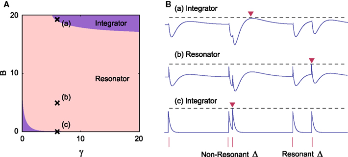
Figure A1. (A) Parameter range in which our augmented MAT model behaves as a resonator, with γ = τ_β / ττ_m and B = βτβ_m. (B) Three sample dynamics of V(t) − θ(t) (blue traces) in response to current pulse inputs (red bars), including two pairs of pulses with different inter-pulse intervals Δ. They correspond to the points of (a), (b), and (c) in A, respectively. The dashed line represents the maximum value of V(t) − θ(t). Each red inverted triangle represents the possible spike that may appear if V(t) reaches θ(t). In the case of (b), the model can emit a spike only for a limited range of Δ value.