Low-level contrast statistics are diagnostic of invariance of natural textures

Introduction

Despite the complexity and variability of everyday visual input, the human brain rapidly translates light falling onto the retina into coherent percepts. One of the relevant features to accomplish this feat is texture information (Bergen and Julesz, 1983; Malik and Perona, 1990; Elder and Velisavljević, 2009). Texture—“the stuff in the image” (Adelson and Bergen, 1991)—is a property of an image region that can be used by early visual mechanisms for initial segmentation of the visual scene into regions (Landy and Graham, 2004), to separate figure from ground (Nothdurft, 1991) or to judge 3D shape from 2D input (Malik and Rosenholtz, 1997; Li and Zaidi, 2000). The relevance of texture for perception of natural images is demonstrated by the finding that a computational model based on texture statistics accurately predicted human natural scene categorization performance (Renninger and Malik, 2004).

In general, a desirable property for any visual feature is perceptual invariance to common viewing variations such as illumination and viewing angle. Whereas invariance is often defined at the level of cognitive templates (e.g., Biederman, 1987) or as a “goal” of visual coding that needs to be achieved by multiple consecutive transformation along the visual pathway (Riesenhuber and Poggio, 1999; DiCarlo and Cox, 2007), there is another possible interpretation: invariance may also be present to a certain degree in the natural world. Specifically, it can be hypothesized that textures that are more invariant will provide more reliable cues for object and scene perception.

The effects of viewing conditions on textures have been previously studied by Geusebroek and Smeulders (2005), who showed that changes in image recording conditions of natural materials are well characterized as changes in underlying contrast statistics. Specifically, two parameters fitted to the contrast histogram of natural images described the spatial structure of several different materials completely. These parameters express the width and outline of the histogram (Figure 1A) and carry information about perceptual characteristics of natural textures such as regularity and roughness (Geusebroek and Smeulders, 2005).

FIGURE 1

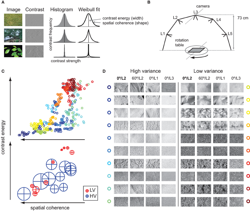
Figure 1. Contrast statistics of natural images. (A) Contrast histograms of natural images follow a Weibull distribution. Three natural images with varying degrees of details and scene fragmentation are displayed as well as a contrast-filtered (non-rectified) version of the same image. The homogenous, texture-like image of grass (upper row) contains many contrasts of various strengths; its contrast distribution approaches a Gaussian. The strongly segmented image of green leaves against a uniform background (bottom row) contains very few, strong contrasts that are highly coherent; its distribution approaches power law. Most natural images, however, have distributions in between (middle row). The degree to which images vary between these two extremes is reflected in the free parameters of a Weibull fit to the contrast histogram. The first parameter describes the width of the histogram: it varies roughly with the distribution of local contrast strengths, a property that we call contrast energy. The second parameter describes the shape of the histogram: it varies globally with the amount of scene clutter, which we call spatial coherence. (B) The texture images were photographs of natural materials (e.g., wool, sand, bread) taken while rotation and illumination angle were manipulated. The materials were placed on a turntable, and recordings were made for aspects of 0, 60, 120, and 180°; for each rotation, the material was illuminated by switching one of five different light sources (L1–L5) on in turn. Technical details are listed on http://staff.science.uva.nl/~aloi/public_alot/ (C) Top: The 400 texture images (20 images for each texture material, i.e., category) set out against their contrast statistics parameters contrast energy and spatial coherence; high-variant (HV) stimuli are colored in shades of blue to green, whereas low-variant (LV) stimuli are in shades of yellow to red. Bottom: Mean and standard deviation in contrast parameters per texture category; HV images in blue, LV images in red. (D) Example images for each of the 20 texture categories that were used for experimentation: per category, an example is shown for a 60° change in rotation, and for a change from middle to side or top illumination angle (L2 to L1/L3).

Recently, we found that for a set of natural images, the same statistics explain up to 80% of the variance of event-related potentials (ERPs) recorded from visual cortex (Ghebreab et al., 2009). We proposed that the two contrast parameters reflect relevant perceptual dimensions of natural images, namely the amount of contrast energy and spatial coherence in a scene. Importantly, we found that these parameters can be reliably approximated by linear summation of the output of localized contrast filters modeled after LGN cells (Scholte et al., 2009), suggesting that these statistics may be available to visual cortex directly from its pre-cortical contrast responses.

In the present work, we evaluated contrast statistics of a large set of natural textures that were recorded under different viewing conditions (Geusebroek and Smeulders, 2005). The contrast energy and spatial coherence of a substantial amount of textures covaried with viewing conditions. However, the statistics of some textures remained remarkably constant under these variations. If the visual system is indeed highly sensitive to variability in low-level image statistics, differences between textures in terms of this variability should have a consequence for their perceptual processing. Specifically, textures with constant contrast statistics across differences in viewing conditions may form more invariant representations compared to other textures.

To test this hypothesis, we asked whether perceptual invariance (experiment 1 and 2) and invariance in evoked neural responses (experiment 3) to natural textures under changes in viewing conditions was associated with variance in contrast statistics. We selected images of multiple textures that differed in two recording conditions: illumination angle and rotation (Figure 1B). Based on variance in contrast statistics, textures were labeled as either “HV” or “LV,” Figure 1C; example images of each texture category are shown in Figure 1D. In experiment 1, human observers performed a same-different categorization task on pairs of images that were either from the same or a different texture category. We tested whether variance in contrast statistics influenced categorization accuracy: we predicted that compared to HV textures, images from the same LV texture would appear more similar (i.e., higher accuracy of same-texture trials) and would also be less often confused with other textures (higher accuracy on different-texture trials), indicating higher “perceived invariance.” In experiment 2, we addressed the same question using another behavioral paradigm—an oddity task—in which participants selected one of three images belonging to a different texture category. We predicted that when presented with two texture images from the same HV category, participants would more often erroneously pick one of these images as the odd-one-out, indicating less “perceived invariance” on these trials. In experiment 3, event-related EEG responses (ERPs) to individually presented texture images were collected and used to examine differences in neural processing between HV and LV textures and to evaluate the contribution of each of the two image parameters (contrast energy and spatial coherence) over the course of the ERP. Specifically, we related differences in image statistics to differences in single-image responses; an avenue that more researchers are beginning to explore (Philiastides and Sajda, 2006; Scholte et al., 2009; van Rijsbergen and Schyns, 2009; Gaspar et al., 2011; Rousselet et al., 2011). The advantage of this approach relative to traditional ERP analysis (which is based on averaging many trials within a condition or an a priori-determined set of stimuli) is that it provides a richer and more detailed impression of the data and that it allows us to examine how differences between individual images can give rise to categorical differences in a bottom-up way.

The results show that variance in contrast statistics correlates with perceived texture similarity under changes in rotation and illumination, as well as differences in neural responses due to illumination changes. They suggest that low-level contrast statistics are informative about the degree of perceptual invariance of natural textures.

Materials and Methods

Computation of Image Statistics

Contrast filtering

We computed image contrast information according to the standard linear-nonlinear model. For the initial linear filtering step we used contrast filters modeled after well-known receptive fields of LGN-neurons (Bonin et al., 2005). As described in detail in Ghebreab et al. (2009) each location in the image was filtered with Gaussian second-order derivative filters spanning multiple octaves in spatial scale, following Croner and Kaplan (1995). Two separate spatial scale octave ranges were applied to derive two image parameters. For the contrast energy parameter, each image location was processed by filters with standard deviations 0.16, 0.32, 0.64, 1.28, 2.56 in degrees; for the spatial coherence parameter, the filter bank consisted of octave scales of 0.2, 0.4, 0.8, 1.6, and 3.2°. The output of each filter was normalized with a Naka-Rushton function with five semi-saturation constants between 0.15 and 1.6 to cover the spectrum from linear to non-linear contrast gain control in the LGN (Croner and Kaplan, 1995).

Response selection

From the population of gain- and scale-specific filters, one filter response was selected for each location in the image using minimum reliable scale selection (Elder and Zucker, 1998): a spatial scale control mechanism in which the smallest filter with output higher than what is expected to be noise for that specific filter is selected. In this approach (similar steps are implemented in standard feed-forward filtering models, e.g., Riesenhuber and Poggio, 1999) a scale-invariant contrast representation is achieved by minimizing receptive field size while simultaneously maximizing response reliability (Elder and Zucker, 1998). As previously (Ghebreab et al., 2009), noise thresholds for each filter were determined in a separate set of images (a selection of 1800 images from the Corel database) and set to half a standard deviation of the average contrast present in that dataset for a given scale and gain.

Approximation of Weibull statistics

Applying the selected filter at each to location to the image results in a contrast magnitude map. Based on the different octave filter banks, one contrast magnitude map was derived for the contrast energy parameter and one for the spatial coherence parameter. These contrast maps were then converted into two 256-bin histograms. It has been demonstrated that contrast distributions of most natural images adhere to a Weibull distribution (Geusebroek and Smeulders, 2002). The Weibull function is given by:

$\begin{array}{cc}p(r)={\text{ce}}^{{\left(\frac{r-\mu }{\beta }\right)}^{\gamma }}& (1)\end{array}$

where c is a normalization constant and μ, β, and γ are the free parameters that represent the origin, scale and shape of the distribution, respectively. The value of the origin parameter μ is generally close to zero for natural images. The contrast energy parameter (β) varies with the range of contrast strengths present in the image. The spatial coherence parameter (γ) describes the outline of the distribution and varies with the degree of correlation between local contrast values.

As mentioned, these two parameters can also be approximated in a more biologically plausible way: we demonstrated that simple summation of X- and Y-type LGN output corresponded strikingly well with the fitted Weibull parameters (Scholte et al., 2009). Similarly, if the outputs of the multi-scale, octave filter banks (Ghebreab et al., 2009) used here—reflecting the entire range of receptive field sizes of the LGN—are linearly summed, we obtain values that correlate even stronger with the Weibull parameters obtained from the contrast histogram at minimal reliable scale (Ghebreab et al., under review). In the present stimulus set, the approximation based on summation of the two filter banks correlated r = 0.99 and r = 0.95 with respectively the beta and gamma parameter of a Weibull function fitted to the contrast histogram. For all analyses presented here, these biologically realistic approximations based on linear summation were used instead of the fitted parameters.

Experiment 1: Behavioral Categorization with a Same-Different Task

Subjects

In total, 28 subjects participated in the first behavioral categorization experiment. The experiment was approved by the ethical committee of the University of Amsterdam and all participants gave written informed consent prior to participation. They were rewarded for participation with either study credits or financial compensation (7€ for one hour of experimentation). The data from two participants was excluded because mean behavioral performance was at chance level (50%).

Stimuli

Texture images were selected from a large database of natural materials (throughout the document, we will refer to these as “texture categories,” http://staff.science.uva.nl/~aloi/public_alot/) that were photographed under various systematic manipulations (illumination angle, rotation, viewing angle, and illumination color). For the subset used in the present study, images (grayscale, 512 × 342 pixels) of each texture category varied only in illumination angle (five different light sources) and rotation (0, 60, 120, or 180°), while viewing angle (0° azimuth) and illumination color (white balanced) were held constant. This selection yielded 20 unique images per texture category. For all 250 categories in the database, contrast statistics were computed for this subset of images. Based on the resulting contrast energy and spatial coherence parameters, textures were designated as either HV or LV if the variance in both parameter values was more than 0.5 standard deviation above (HV) or below (LV) the median variance for all textures. From those two selections, 10 texture categories were randomly chosen; however, care was taken that the mean parameter values of the selected categories were representative of the range of the entire database. The final selection thus yielded 20 texture categories, 10 of which formed the “HV condition” and 10 that formed the “LV condition,” with each category consisting of 20 images that were systematically manipulated in illumination angle and rotation. Thus, in total, 400 images were used for experimentation.

Procedure

On each trial, two images were presented which were from the same or a different texture category. Stimuli were presented on a 19 inch Dell monitor with a resolution of 1280 × 1024 pixels and a frame rate of 60 Hz. Participants were seated approximately 90 cm from the monitor and completed four blocks of 380 trials each. A block contained four breaks, after which subject could continue the task by means of a button press. On each trial, a fixation cross appeared on the center of the screen; after an interval of 500 ms, a pair of stimuli was presented simultaneously for 50 ms, separated by a gap of 86 pixels (Figure 2A). A mask (see below) followed after 100 ms, and stayed on screen for 200 ms. Subjects were instructed to indicate if the stimuli were from the same or a different texture category by pressing one of two designated buttons on a keyboard (“z” and “m”) that were mapped to the left or the right hand. Within one block, one stimulus from one texture category was once paired with a stimulus from another texture category (190 trials). Stimuli were drawn without replacement, such that each image occurred once in each block, but were randomly paired with the images from the other texture category on each block. For the other 190 trials, the two stimuli were from the same texture category: for each texture category, 10 pairs were randomly chosen, resulting in 200 trials (20 from each texture category), from which 10 were then randomly removed (but never more than one from each category) such that 190 trials remained. The ratio of different-category vs. same-category comparisons was thus 1, which was explicitly communicated to the subjects prior to the test phase. Subjects were shown a few example textures, which contained examples of both illumination and rotation changes, and they also performed 20 practice trials before starting the actual experiment (none of these examples occurred in the experiment; the practice trials contained comparisons of both illumination and rotation changes between the two presented texture images). Masks were created by dividing each of the 400 texture stimuli up in mini-blocks of 9 × 16 pixels: a mask was created by drawing equal amounts of these mini-blocks from each stimulus and placing those at random positions in a frame of 512 × 342 pixels. Unique masks were randomly assigned to each of the 400 trials within a block, and were repeated over blocks. Per trial, the same mask was presented at both stimulus locations. Stimuli were presented using Matlab Psychophysics Toolbox (Brainard, 1997; Pelli, 1997).

FIGURE 2

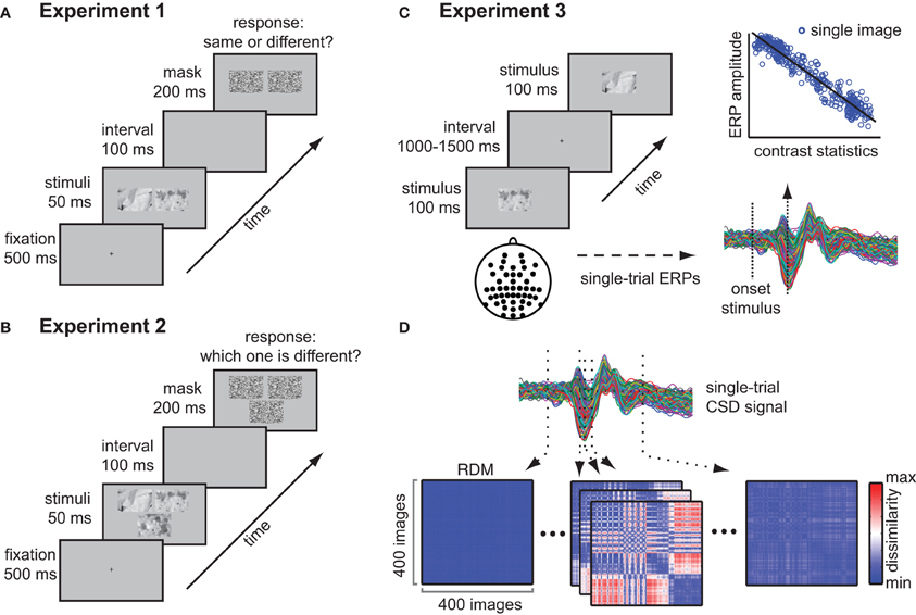
Figure 2. Methods and experimental design. (A) Experimental paradigm of experiment 1 (behavioral same-different task). Participants performed a same-different categorization task on pairs of texture stimuli that were presented on a gray background and that were masked after 200 ms. (B) Experimental paradigm of experiment 2 (behavioral oddity task); participants chose the odd-one-out from three images on each trial. (C) Experimental set-up and analysis of experiment 3 (single image presentations). Subjects were presented with individual texture images while electroencephalogram (EEG) was recorded. Single-image evoked responses were computed for each electrode, after which a regression analysis of the amplitude at each time-point based on contrast statistics was performed. (D) Representational dissimilarity matrices (RDMs) were computed at each sample of the CSD-transformed ERP recorded from channel Oz. A single RDM displays dissimilarity (red = high, blue = low, reflecting difference in ERP amplitude) between all pairs of stimuli at a specific moment in time.

Data analysis

Mean accuracy for each subject was determined by calculating percent correct over four repeated blocks and was done separately for different-category vs. same-category comparisons and for trials on which two HV categories were compared vs. trials on which two LV categories were compared (2 × 2 design). Different-category trials on which HV categories were compared to LV categories were excluded from analysis. Only the responses, and not the reaction times (RTs) were recorded: as a consequence a number of trials in which subjects may have responded too fast (for instance before 200 ms) were included in the analysis. This results in a potential underestimation of the error rate.

Experiment 2: Behavioral Categorization with an Oddity Task

Subjects

In total, 18 subjects participated in the second behavioral categorization experiment, which was approved by the ethical committee of the University of Amsterdam. All participants gave written informed consent prior to participation. They were rewarded for participation with either study credits or financial compensation (7€/hour), as previously. The data from two participants was excluded because mean performance was at chance level (33%, one participant) or because RTs demonstrated an outlier (>2 standard deviations away from the mean across all participants, one participant).

Stimuli and procedure

The same set of 400 texture images was used as in the first behavioral experiment. However, for this task, on each trial three images were presented: two images from the same texture category (the “same pair”), and one from a different category (the “odd-one-out”), see Figure 2B. Stimuli were presented on a 19-inch ASUS monitor with a resolution of 1920 × 1080 pixels and a frame rate of 60 Hz. The procedure was identical to the first behavioral experiment, i.e., the stimuli were presented simultaneously: in this case, two images were positioned adjacent to each other and the third image was located either below or above the other two (this was counterbalanced across participants). The three images were separated by equal gaps of 120 pixels. The position of the odd stimulus was randomized over trials. Subjects were instructed to indicate which image was from the different texture category by pressing one of three designated buttons on a keyboard (“1”, “2”, and “3” on the NUM pad of the keyboard) using their right hand. Within one block, each texture category was twice paired with every other texture category by randomly drawing a stimulus from both categories (380 trials). For one half of the trials, the image from the first category was designated as the “odd-one-out,” whereas from the second category, another stimulus was drawn to form the second half of the “same pair.” For the other half of the trials, the procedure was reversed, such that each texture category once formed the odd stimulus, and once formed the paired stimulus. Compared to the first experiment, the trials were thus always “different-category trials,” but on a given trial, each texture category could be the odd stimulus or the same-pair stimulus, allowing us to test whether variance of the same-pair texture images influenced performance: we predicted that increased variance in contrast statistics of the same-pair stimuli would lead to more errors (i.e., selecting one of the same-pair as the odd-one-out).

Data analysis

As in the first experiment, except that trials in which the participant responded before 200 ms after stimulus-onset were excluded. To allow comparison with the same-different accuracy data from the previous experiment, we first selected only the trials on which either two HV or two LV texture categories were compared (ignoring trials on which one HV and one LV category were compared). The same comparison was done for RTs. In a subsequent analysis, we did include all trials but split them into two groups in two different ways: namely (1) based on whether the odd stimulus was LV or HV or (2) based on whether the same-pair were HV or LV. This allowed us to test whether the variance of the odd stimulus vs. the variance of the same-pair was associated with increased error rates in selection of the odd stimulus.

Experiment 3: EEG Experiment

Subjects

Seventeen volunteers participated and were rewarded with study credits or financial compensation (7€/hour for 2,5 h of experimentation). The data from two subjects was excluded because the participant blinked consistently shortly after trial onset in more than 50% of the trials (one subject) of because their vision deviated from normal (one subject) which became clear in another experiment conducted in the same session. This study was approved by the ethical committee of the University of Amsterdam and all participants gave written informed consent prior to participation.

EEG data acquisition

The same set of stimuli was used as in the behavioral experiment. In addition, for each image a phase-scrambled version was created, which were presented randomly intermixed with the actual textures, with equal proportions of the two types of images. Stimuli were presented on an ASUS LCD-screen with a resolution of 1024 × 768 pixels and a frame rate of 60 Hz. Subjects were seated 90 cm from the monitor such that stimuli subtended 11 × 7.5° of visual angle. During EEG acquisition, a stimulus was presented one at a time in the center of the screen on a gray background for 100 ms, on average every 1500 ms (range 1000–2000 ms; Figure 2C). Each stimulus was presented twice, in two separate runs. Subjects were instructed to indicate on each trial whether the image was an actual texture or a phase-scrambled image: a few examples of the two types of images were displayed prior to the experiment. Response mappings were counterbalanced between the two separate runs for each subject. Stimuli were presented using the Presentation software (www.neurobs.com). EEG Recordings were made with a Biosemi 64-channel Active Two EEG system (Biosemi Instrumentation BV, Amsterdam, NL, http://www.biosemi.com/) using the standard 10–10 systems with additional occipital electrodes (I1 and I2), which replaced two frontal electrodes (F5 and F6). Eye movements were monitored with a horizontal and vertical electro-oculogram (EOG) and were aligned with the pupil location when the participants looked straight ahead. Data was sampled at 256 Hz. The Biosemi hardware is completely DC-coupled, so no high-pass filter is applied during recording of the raw data. A Bessel low-pass filter was applied starting at 1/5th of the sample rate.

EEG data preprocessing

The raw data was pre-processed using Brain Vision Analyzer (BVA) by taking the following steps: (1) offline referencing to earlobe electrodes, (2) applying a high-pass filter at 0.1 Hz (12 dB/octave), a low-pass filter at 30 Hz (24 dB/octave); because low-pass filters in BVA have a graded descent, additionally two notch filters at 50 (for line noise) and 60 Hz (for monitor noise) were applied, (3) automatic removal of deflections larger than 250 μV. Trials were segmented into epochs starting 100 ms before stimulus onset and ending 500 ms after stimulus onset. These epochs were corrected for eye movements by removing the influence of ocular-generated EEG using a regression analysis based on the EOG channels (Gratton et al., 1983). Baseline correction was performed based on the data between −100 and 0 ms relative to stimulus onset; artifacts were rejected using maximal allowed voltage steps of 50 μV, minimal and maximal allowed amplitudes of −75 and 75 μV and a lowest allowed activity of 0.50 μV. The resulting ERPs were converted to Current Source Density (CSD) responses (Perrin, 1989). This conversion results in a signal that is more localized in space, which has the advantage of more reliably reflecting activity of neural tissue underlying the recording electrode (Nunez and Srinivasan, 2006). Trials in which the same individual image was presented were averaged over the two runs, resulting in an image-specific ERP (single-image ERP).

Regression analyses on single-image ERPs

To test whether differences between neural responses correlated with differences in contrast statistics between images, we conducted regression analyses on the single-image ERPs (Figure 2C). We first performed this analysis on ERPs averaged across subjects to test whether contrast energy and spatial coherence could explain consistent differences between images. For each channel and time-point, the image parameters (contrast energy and spatial coherence) were entered together as linear regressors on ERP amplitude, resulting in a measure of model fit (r²) over time (each sample of the ERP) and space (each electrode). To statistically evaluate the specific contribution of each parameter to the explained variance for the two different image conditions (HV en LV), we ran regressions at the single subject level (these analyses were restricted to electrode Oz). For this, we constructed a model with four predictors of interest (constant term + LV contrast energy, HV contrast energy, LV spatial coherence, HV spatial coherence). The obtained β-coefficients for each predictor were subsequently tested against zero by means of t-tests, which were Bonferroni-corrected for multiple comparisons based on the number of time-points for which the comparison was performed (154 samples). Finally, to test whether each predictor contributed unique variance, we conducted a stepwise version of the two-parameter (contrast energy and spatial coherence for both LV and HV images) regression analysis for each single subject. In this analysis, a predictor was entered to the model if it was significant at α < 0.05, and was removed again if α > 0.10; as an initial model, none of the parameters were included. We then counted, at every time-point, for how many subjects the full model was chosen, or only one of the predictors was included.

Representational similarity analysis

To better examine how variance between individual visual stimuli arises over time, and how differences between individual images relate to image variance (HV/LV) and image manipulations (rotation/illumination), we computed representational dissimilarity matrices (RDMs; Kriegeskorte et al., 2008) based on single-image ERPs recorded at channel Oz. We computed, for each subject separately, at each time-point, for all pairs of images the difference between their evoked ERP amplitude (Figure 2D). As a result we obtained a single RDM containing 400 × 400 “dissimilarity” values between all pairs of images at each time-point. Within one such matrix, the pixel value of each cell reflects the difference in ERP amplitude of the corresponding two images indicated by the row- and column number.

Comparison between dissimilarity matrices

To compare the dissimilarities between evoked ERPs by individual images with corresponding differences in image statistics between those images, we computed a pair-wise dissimilarity matrix based on both image parameter values combined. For each pair of images, we computed the sum of the absolute differences between the (normalized) contrast energy (CE) and spatial coherence (SC) values of those two images [e.g., (CE_image1 + SC_image1) − (CE_image2 + SC_image2), etc.], resulting in one difference value reflecting the combined difference in image parameters between the two images. For each subject, this matrix was compared with the RDMs based on the ERP data using a Mantel test for two-dimensional correlations (Daniels, 1944).

Computation of luminance and AIC-values

To obtain a simple description of luminance for each image, we computed the mean luminance value per image (LUM) by averaging the pixel values (0–255) of each individual image. For the EEG analysis, to compare the regression results based on LUM with those obtained with contrast statistics, we used Akaike's information criterion (AIC; Akaike, 1973). The AIC-values were computed by transforming the residual sum of squares (RSSs) of each regression analysis using

$\begin{array}{cc}\text{AIC}=n*\text{log}(\text{RSS}/n)+2k& (2)\end{array}$

where n = number of images and k is the number of predictor variables (k = 2 for contrast statistics, and k = 1 for LUM). AIC can be used for model selection given a set of candidate models of the same data; the preferred model has minimum AIC-value.

Results

Experiment 1: Same-Different Categorization

Categorization accuracy was determined separately for HV and LV trials and for same-category and different-category comparisons (Figure 3A). A repeated-measures, two-way ANOVA indicated a significant main effect of variance [F_{(1, 25)} = 298.9, p < 0.0001], but not of type of comparison [F_{(1, 25)} = 3.6, p = 0.07]; however, there was a significant interaction between variance and comparison [F_{(1, 25)} = 61.8, p < 0.0001; Figure 3B]. Subsequent paired t-tests revealed that participants performed better for LV than HV textures at both different-category [t₍₂₅₎ = 6.1, p < 0.0001, mean difference = 6%, ci = 4–8%] and same-category comparisons [t₍₂₅₎ = 16.3, mean difference = 17%, ci = 15–19%, p < 0.0001], but also for different-category HV comparisons relative to same-category HV comparisons [t₍₂₅₎ = 3.4, mean difference = 11%, ci = 4–17%, p = 0.002]. These results show that participants generally made more errors on trials in which they compared two different HV texture categories than on trials which consisted of two LV texture categories; in addition, they more often incorrectly judged two images from the same HV texture category as different than vice versa (two different HV images as the same category). This finding suggests that LV texture categories are easier to categorize than HV texture categories and that images from the same HV texture category are perceived as less similar. This latter conclusion is supported by an additional analysis performed on the accuracy scores, in which we correlated the specific amount of variance in contrast statistics with the average number of same-texture errors. We found that variance in contrast statistics correlated with same-texture accuracy across all texture categories (Spearman's ρ = −0.73, p < 0.0001, Figure 3C). This result suggests that the specific amount of variance in contrast statistics influences perceived similarity of same-texture images: more variance implies less similarity.

FIGURE 3

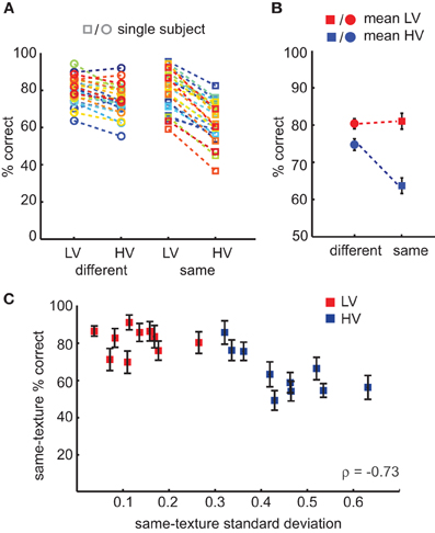
Figure 3. Results of the behavioral same-different experiment. (A) Accuracy scores for individual subjects according to task conditions: subjects compared a pair of images that were either from different (circles) or same (squares) texture categories, which could either be low-variant or high-variant. Trials in which HV images were compared with LV images were excluded from the analysis. (B) Mean accuracy per condition, demonstrating an interaction effect between texture variance (HV, blue vs. LV, red) and type of comparison (same vs. different trial). (C) Accuracy on same-texture trials correlates with category specific variance in contrast statistics. Error bars indicate s.e.m.

As subjects always compared only two images on each trial, we cannot be certain to what degree they based their judgment on the between-stimulus differences vs. the difference of these two images compared to all other images in the stimulus set. To investigate this more explicitly, we conducted another behavioral experiment using an oddity task, in which each trial consisted of three images that were drawn from two different texture categories. In this task, subjects always make a difference judgment: they have to pick the most distinct stimulus (the “odd-one-out”) and thus actively compare differences between texture categories with differences within texture categories. If variance in contrast statistics of a texture category indeed determines its perceived invariance, we would expect that for comparisons between images with high variance, it is more difficult to accurately decide which stimulus is different.

Experiment 2: Oddity Categorization

Categorization accuracy on comparisons of HV texture categories was significantly lower compared to comparisons of LV texture categories [t₍₁₅₎ = 14.4, mean difference = 17%, ci = 14–20%, p < 0.0001]; Figure 4A. Participants were also significantly faster on LV trials compared to HV trials [t₍₁₅₎ = −3.5, mean difference = 27 ms, ci = 10–43 ms, p < 0.004]. If we compute accuracy across all possible comparisons of texture categories (also including HV-LV comparisons), and split the data either according to the variance of the odd stimulus, or to the variance of the same-pair stimulus on each trial, we see that specifically the variance of the same-pair images is correlated with differences in accuracy (Figure 4B): on trials at which the same-pair was from a HV texture category, subjects more often incorrectly chose one of that pair as the odd-one-out. As in the previous experiment, we correlated the amount of variance in contrast statistics of the same-pair with accuracy, and we again find a significant correlation (ρ = −0.75, p < 0.0001; Figure 4C), indicating that with increasing variance in contrast statistics, images from the same texture category are more often perceived as different.

FIGURE 4

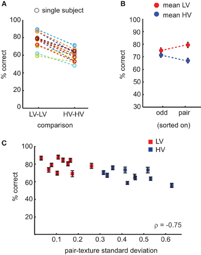
Figure 4. Results of the behavioral oddity experiment. (A) Accuracy scores for individual subjects for comparisons between HV categories or between LV categories: subjects more often erroneously picked one of the “same-pair” stimuli as the odd-one-out if they were from a HV texture category. (B) Mean accuracy across all trials (including trials in which HV images were compared with LV images) sorted either according to the odd stimulus condition (HV/LV) or the same-pair condition, demonstrating that the condition of the same-pair correlates with accuracy, not the identity of the odd-one-out. (C) The variance of the same-pair correlates with category specific variance in contrast statistics. Error bars indicate s.e.m.

Overall, the results of the two behavioral experiments indicate that low variance in contrast statistics allows observers to more accurately categorize images of natural textures. Importantly, images of a texture category with constant statistics under different viewing conditions are more accurately recognized as the same category compared to images from categories with variable statistics, suggesting that textures categories with little variance in contrast statistics are perceived as more invariant.

Experiment 3: EEG

Contrast statistics explain variance in occipital ERP signals

As a first-pass analysis, we first averaged single-image ERPs over subjects, after which a simple regression model with two predictors (contrast energy and spatial coherence) was fitted based on these “subject-averaged” ERPs at every channel and time-point. Despite individual differences between subjects in EEG responses (e.g., in mean evoked response amplitude, likely due to individual differences in cortical folding), this analysis revealed a highly reliable ERP waveform time-locked to the presentation of the stimulus (Figure 5A). This time-locked ERP nonetheless varied substantially between individual images, mostly between 100 and 300 ms after stimulus-onset. The results show that early in time, nearly all ERP variance is explained by the image parameters (maximal r² = 0.94 at 148 ms, p < 0.0001 on channel Oz, Figure 5B). Also at later time-points and at other electrodes, there is substantial (e.g., more than 50%) explained variance. If we examine the results for all channels simultaneously (Figure 5C), we see that explained variance is highest at occipital channels, and subsequently wears off toward more parietal and lateral electrodes. This localization is similar for both early and late time-points (i.e., mostly central-occipital).

FIGURE 5

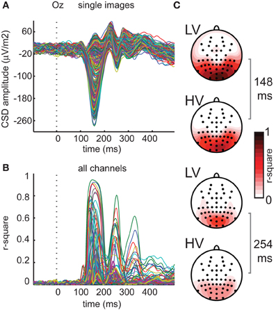
Figure 5. Regression analyses on mean ERP data for all channels. (A) Individual image ERPs converted to current source density signals (CSDs) averaged over subjects at channel Oz. (B) Explained variance at each time-point resulting from regression analyses of mean ERP amplitude on contrast statistics of the 400 texture images (average of two presentations) at all 64 electrodes. (C) Results of regression analysis based on mean ERP for all electrodes, at two time-points of peak explained variance (148 and 254 ms), indicating substantial explained variance on electrodes overlying visual cortex for both high-variant (HV) and low-variant (LV) texture categories.

This result shows that low-level image statistics can explain a high amount of variance, both early and late in time, of image-specific differences across participants. To test more precisely (1) whether these effects were present in all participants, (2) which of the two image parameters contributed most to the explained variance, and (3) whether these contributions differed between the two conditions (LV/HV), we selected the electrode with the highest r²-value (Oz) and conducted regression analyses at the single-subject level using a model containing four parameters (see Materials and Methods): LV contrast energy, HV contrast energy, LV spatial coherence, HV spatial coherence. The results showed that contrast statistics explained a substantial amount of variance between individual images in each participant. Mean explained variance across subjects peaked 156 ms after stimulus onset (r² = 0.65, mean p < 0.0001, Bonferroni-corrected; Figure 6A); peak values for individual subjects ranged between r² = 0.49–0.85 at 144–168 ms after stimulus-onset and were all highly significant (all p < 0.0001).

FIGURE 6

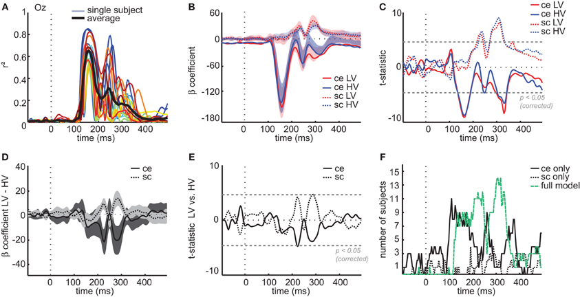
Figure 6. Regression analyses on single-subject ERP data at channel Oz. (A) Explained variance at channel Oz for each individual subject (colored lines) and averaged across subjects (black line) based on a regression model with four predictors (see Materials and Methods) (B) Mean β-coefficient at each time-point associated with each of the four predictors; ce, contrast energy; sc, spatial coherence; LV, low-variant; HV, high-variant. Shaded areas display confidence intervals obtained from a t-test of each predictor against zero across single subjects. (C) Resulting t-statistic of testing the β-coefficient associated with each predictor against zero for every time-point of the ERP: the gray dashed line indicates significance level at α < 0.05 when correcting for multiple comparisons (Bonferroni-correction). (D) Difference in mean β-coefficients between LV and HV images for each image parameter. Shaded areas display confidence intervals obtained from a t-test between LV and HV coefficients across single subjects. (E) Resulting t-statistic of the difference between LV and HV coefficients: gray dashed line indicates Bonferroni-corrected significance level at α < 0.05. (F) Results of the single-subject stepwise regression analysis: displayed are the number of subjects for which either only contrast energy (black solid line), only spatial coherence (black dotted line) or both parameters (green dashed line) were included in the model at each time-point of the ERP.

If we compare the time courses of the β-coefficients associated with each predictor (Figure 6B), we observe that contrast energy and spatial coherence have distinct time courses. Statistical comparisons of each coefficient against zero across participants (Figure 6C) show that ERP amplitude at an early time interval is mostly correlated with contrast energy [between 136 and 183 ms, all t₍₁₅₎ < −5.1, max t₍₁₅₎ = −9.0, all p < 0.0003], which correlates again much later in time [between 305 and 340 ms, all t_{(15) < −5.1}, max t₍₁₅₎ = −6.5, all p < 0.0001]. Spatial coherence only contributes significantly to the explained variance between 220 and 240 ms, [all t₍₁₅₎ > 4.7, max t₍₁₅₎ = 6.1, all p < 0.003; again between 274 and 330 ms, all t₍₁₅₎ > 5.4, max t₍₁₅₎ = 9.0, all p < 0.0003]. Importantly, at most time-points the temporal profile of each predictor is comparatively similar for HV and LV images; differences between the beta coefficients of these two conditions are relatively small (Figure 6D). For both image parameters, the difference between HV and LV images appears to be substantial only at two time-intervals between 150 and 300 ms, but statistical tests of these differences were right at the threshold of Bonferroni-corrected significance [contrast energy at 223 ms, t₍₁₅₎ = −4.8, p = 0.0002; spatial coherence, at 285 and 289 ms, t₍₁₅₎ = 4.6, p = 0.0003; Figure 6E]. Given the small effects and the borderline significance, this issue cannot be resolved with the current dataset.

Finally, to test whether the two image parameters explain unique variance, we conducted stepwise regression analyses (see Materials and Methods) based on evoked responses of single subjects on ERPs recorded at channel Oz. At each time-point of the ERP, we counted for how many participants (a) either the full model was chosen or (b) only one predictor was included in the model (Figure 6F). The results show that early in time, the contrast energy parameter alone is preferred over the full model, but that later in time (from ~200 ms onwards), for most subjects the spatial coherence parameter is also included. This suggests that especially later in time, spatial coherence adds additional explanatory power to the regression model.

These results show that across subjects, differences in early ERP amplitude between individual images correlate with variance in contrast statistics of those images for both HV and LV textures. Whereas contrast energy explains most variance early in time, both parameters become significantly correlated with ERP amplitude at later time intervals. These regression results do not reveal, however, whether these differences are related to texture category (categorical differences), or if they occur as a result of variations in recording conditions. We investigated this in the next section.

Dissimilarities between images map onto contrast statistics

To examine the origin of the variance between individual trials, we computed (for each subject separately) RDMs based on differences in evoked responses between individual images (see Materials and Methods and Figure 2D). In brief, to build an RDM, we compute for each possible combination of individual images the difference in evoked ERP amplitude, and convert the result into a color value. The advantage of this approach is that RDMs allow us to see at once how images are (dis)similar to all other images, and how this relates to texture category “membership.”

To demonstrate the result of this analysis, we selected the RDM at the time-point of maximal explained variance for the subject-averaged regression analysis (148 ms after stimulus-onset) for each subject and simply averaged the resulting matrix over subjects. In this RDM (Figure 7A), every consecutive 20 rows/columns index all images from one specific texture category; these categories are sorted according to their mean contrast energy and spatial coherence values (i.e., distance from zero in the contrast statistics space in Figure 1C). If we visually examine the RDM, we observe that differences between HV images (lower right quadrant) occur at different positions than for LV images (upper left quadrant). Specifically, for HV stimuli, there are larger differences within textures, whereas for LV stimuli, the differences are largest between textures: i.e., within a 20 × 20 “square,” images are “similarly dissimilar” from other textures. This result suggests that LV images cluster more by texture category than HV images, which are highly different even within a given texture.

FIGURE 7

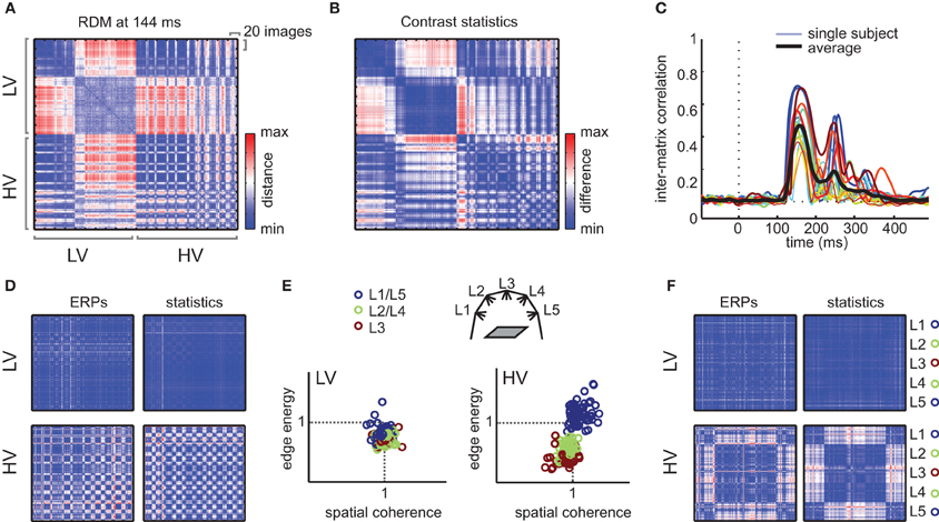
Figure 7. Representational dissimilarity analysis. (A) Mean RDM (averaged over subjects) of the ERP signal at the time-point of maximal dissimilarity. Each cell of the matrix reflects the dissimilarity (red = high, blue = low) between two individual images, whose category is indexed on the x- and y-axis. Starting from the top row, the first 200 images are from LV textures; the other half contains the HV textures, yielding a “LV quadrant” (top left) and a “HV quadrant” (bottom right). Within these quadrants, each consecutive 20 rows/columns index images of a single texture; textures are sorted according to their mean contrast energy and spatial coherence values (distance from the origin in Figure 1C). (B) Dissimilarity matrix based on difference in contrast statistics (combined contrast energy and spatial coherence parameters) between individual images. (C) Correlation between the RDM and contrast statistics dissimilarity matrix (Mantel test) at each sample in time. Both single subject model fits (colored lines) and mean correlations (black line) are shown. (D) The LV and HV quadrants of “demeaned” dissimilarity matrices (for each of the 20 images of one texture category, the mean of those 20 images is subtracted). Left: demeaned quadrants of the RDM based on ERPs. Right: demeaned quadrants of the RDM based on contrast statistics. (E) Demeaned contrast statistics for each image color-coded according to illumination angle (ignoring texture category membership). Illumination angles are illustrated again in the cartoon inset; for color-coding, we collapsed over illumination angle L1 and L5 as well as L2 and L4, which have the same angle but are positioned on opposite sides. (F) The LV and HV quadrants of the demeaned RDMs, but now sorted according to illumination angle, ignoring texture membership. In the HV quadrant only, an effect of illumination is present, visible as clustering of dissimilarities by illumination angle.

Next, we tested to what extent these image-specific differences in ERP amplitude ERP were similar to differences in contrast statistics. We calculated another 400 × 400 difference matrix, in which we simply subtracted the parameter values of each image from the values of each other image (Figure 7B, see Materials and Methods). Based on visual inspection, it is clear that the relative dissimilarities between individual images in contrast statistics are very similar to the ERP differences. A test of the inter-matrix correlation at each time-point (Figure 7C) indicated that the RDM of the ERP signal correlated significantly with the difference matrix based on contrast statistics; between 137 and 227 ms after stimulus onset, the correlation was significant for all 17 subjects (range peak r = 0.31–0.72, all p < 0.01, Bonferroni-corrected).

Dissimilarities between HV stimuli reflect illumination changes

Presumably, the higher dissimilarities within HV textures result from variability in responses driven by changes in recording conditions. To isolate these effects, we computed “demeaned” versions of the RDMs, by dividing the evoked response to each image by the mean response to all 20 images of its texture category, before computing the differences between individual images. As a result, we obtain RDMs that only reflect differences in variance from the mean response to that texture category, ignoring differences between the means of different categories. Analogously, for the contrast statistics matrix, we divided the parameter values between images of a given texture by the mean contrast energy and spatial coherence value of that texture and subsequently computed the image-specific differences.

As one would expect, dissimilarities between images in LV stimuli have completely disappeared in these demeaned RDMs (Figure 7D, displaying only the HV-HC and LV-LV quadrants). This demonstrates that all differences between LV stimuli indeed reflect differences between texture categories. For HV stimuli however, dissimilarities within texture categories remain after demeaning; moreover, we observe a “plaid-like” pattern in the RDM, which suggests that dissimilarities of individual HV images do not fluctuate randomly, but are present in a regular manner. What manipulation is driving these dissimilarities? If we investigate the clustering of images based on demeaned contrast statistics (Figure 7E), we see that for HV stimuli, the variance from the mean is caused by changes in illumination direction: the illumination change “moves” the stimulus to another location the contrast statistics space in a consistent manner. As a final demonstration, we resorted all images in the RDMs based on illumination direction instead of texture category: in the resulting RDM, the differences between ERPs now cluster with illumination changes (Figure 7F), confirming that dissimilarities within HV categories result mostly from illumination differences.

These results again show that differences between individual images in ERP responses are correlated with differences in contrast statistics for those images. Importantly, they reveal that differences between HV textures occur for other reasons than differences between LV textures. For HV textures, we observe that manipulations of illumination angle are reflected in the RDM: instead of clustering by category (which would be evidenced by within-texture similarity and between-texture dissimilarity), images are selectively dissimilar for one illumination angle compared to another. For LV stimuli, the pattern of results is different: stimuli do cluster by category, meaning that all images of a given texture are “similarly dissimilar” from other textures (or similar, if the mean of the other images is very nearby in “contrast statistics space,” Figure 1C). Overall, this suggests that the amount of variance in contrast statistics correlates with variance between neural responses resulting from variations in recording conditions, specifically illumination differences. Textures that vary little in contrast statistics appear to form a more “invariant” representation in terms of evoked responses.

Image manipulations: rotation versus illumination

The results of the EEG experiment suggest that the high variance of HV texture images is related to a higher sensitivity of these textures to changes in illumination direction: the large differences that remain within texture categories after subtracting differences between texture categories appear to be driven by differences in illumination angle. Based on this finding, we can expect that the main result we observed in behavioral categorization (increased error rates on HV texture categories) is also driven by effects of illumination direction, rather than image rotations. To address this question, we post-hoc sorted the data from the same-different experiment based on whether the two presented images differed in (a) rotation only, (b) illumination only, or (c) both rotation and illumination, and separately computed the accuracies for each of the different conditions (same LV, same HV, different LV, different HV). Because the pairing of individual images was randomized over trials (see Materials and Methods), there were unequal amounts of manipulation differences for each subject and condition. To increase the number of trials per condition and to be able to compare across conditions, we collapsed over same angles from different sides, as in the EEG RDM analysis (see Figure 7E, i.e., we counted a pair of images of the same texture category that were illuminated from angle 2/4 or 1/5 as “same illumination”). As a result, we obtained four different “trial-types”: same illumination, same rotation (SI, SR), same illumination, different rotation (SI, DR), different illumination, same rotation (DI, SR), or different illumination, different rotation (DI, DR). The results show that across all trial-types, accuracy is lower for HV than for LV stimuli [Figure 8A; main effect of variance on both same-category and different-category comparisons, all F_{(1, 25)} > 27.9, p < 0.0001]. However, as predicted, on same-category trials most errors are made when illumination is changed compared to when rotation is changed and illumination is kept constant [main effect of illumination, F_{(1, 25)} > 262.9, p < 0.0001]. Importantly, this effect is much larger for the HV texture categories than for the LV texture categories [significant interaction between variance and illumination, F_{(1, 25)} = 162.1, p < 0.0001]. This analysis thus shows that the influence of illumination angles differs for HV vs. LV texture categories: it again demonstrates that the categories from the latter condition are more invariant to these manipulations than other categories. Interestingly, the effect is reversed for different pairs [more errors for same illumination trials; main effect of illumination, F_{(1, 25)} = 20.6, p < 0.0001] suggesting that in this case, illumination changes “help” to distinguish different texture categories more easily. Most importantly, these results support the conclusion that the extent to which a given texture category is sensitive to illumination changes can be derived from contrast statistics.

FIGURE 8

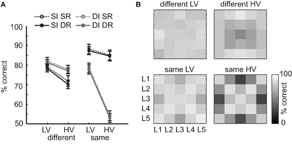
Figure 8. Post-hoc analysis of the effect of image manipulations on accuracy of the same-different categorization experiment. (A) Accuracies for each condition (HV/LV) and type of comparison (same/different) were computed separately for trials in which the two images were either photographed under same illumination and same rotation (SI, SR), same illumination and different rotation (SI, DR), different illumination and same rotation (DI, SR), or different illumination and different rotation (DI, DR). The results show that the participants always made more errors on HV texture categories than LV texture categories: however, this effect is strongest for same-comparison HV trials where there was a difference in illumination angel between images. Error bars indicate s.e.m. (B) Effect of illumination angle (L1–L5, see Figure 1B) on same-illumination (SI, diagonal values) and different-illumination (DI, off-diagonal values) trials (collapsed over SR and DR trials), for each condition and type of comparison. Most errors on same-category HV trials are made for images that have the largest difference in illumination angle (i.e., L3 vs. L1/L5), whereas most errors on different-category HV trials are made for illumination angle L3.

To demonstrate the effects of illumination changes more clearly, we sorted the DI accuracies based on the exact illumination angle (L1–L5, see Figures 1B and 7E) that was used for each of the two presented stimuli on a given trial (given the small effect of rotation, we now collapsed over same rotation and different rotation trial-types, i.e., over SR and DR trials). The results of this analysis are displayed as confusion matrixes in Figure 8B (diagonals represent the SI trials). Here, it can be observed that on same-category HV trials (lower right matrix), most errors are made when the change in illumination angle was large (e.g., a pairing of L3 and L1/L5). For same-category LV trials (lower left matrix), however, this effect is much weaker, indicating that LV texture categories are less responsive to illumination changes. Interestingly, from the confusion matrix of the different category HV trials (upper right panel), it appears that most errors were made when the two different texture images were photographed under angle L3, suggesting that in general, images from different texture categories become more similar when the light is shone right from above; likely, this is due to higher saturation of the image (overexposure) under this illumination angle. This effect is however again absent for the different-category LV trials (upper left panel), suggesting that these saturation effects are less likely to occur for images that are LV in contrast statistics.

Luminance statistics

These behavioral and EEG results suggest that contrast statistics of the texture categories are diagnostic of perceived variance under changes in illumination. The behavioral results further suggest that the amount of illumination change is directly related to the perceived similarity on same-texture HV trials, and that the specific illumination angle used on different-texture HV trials may also influence the observed similarity (Figure 8B). Does this mean that a simple description of differences in luminance between images (i.e., brightness), rather than contrast statistics, would describe the same pattern of results? To test this, we computed the mean luminance (LUM, see Materials and Methods) of each image and tested to what extent differences in luminance were correlated with differences in behavioral categorization and EEG responses.

First of all, LUM values of individual images were indeed highly correlated with contrast energy (ρ = −0.69, p < 0.001), and somewhat lower but significantly correlated with spatial coherence (ρ = −0.38, p < 0.001). However, if we split the texture categories into high and low variance conditions based on LUM values per category, we do not find the same texture categories in each condition as in the original division based on contrast statistics; see Figure 9A. In fact, about half of the LV categories are “HV” in LUM if we separate the categories using a median split. The correlation of variance in LUM and accuracy on same-texture trials was either not significant (ρ = −0.32, p = 0.15, for the oddity experiment) or significant but lower compared to the correlation with contrast statistics (ρ = −0.51, p = 0.02 for the same-different experiment), suggesting that variance in brightness rather than contrast is not an alternative explanation for the finding that observers perceive images from HV texture categories more often as “different.”

FIGURE 9

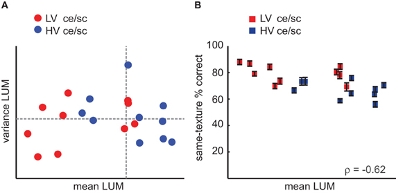
Figure 9. Role of luminance statistics (LUM) in the behavioral data. (A) Mean and variance in LUM for each texture category, still color-coded by variance in contrast statistics (ce/sc; red, LV; blue, HV). Dashed lines indicate the values of the medians. (B) Behavioral accuracy in the oddity experiment on same-texture trials (i.e., same data as in Figure 4C) set out against mean LUM value per texture category, color-coded by variance in contrast statistics. The four “red” texture categories on the right for which accuracy is high would be grouped with the other red categories if the data would be set out against variance in contrast statistics rather than mean LUM values. Error bars indicate s.e.m.

A majority of LV texture categories have low mean LUM values, but this is not the case for all categories, suggesting that HV texture categories are not systematically brighter than LV categories. The correlations of same-texture accuracy and mean LUM per texture category are also inconsistent: significant in the oddity experiment (ρ = −0.62, p < 0.005), but not in the same-different experiment (ρ = −0.35, p = 0.12). As can be seen in Figure 9B, the correlation with behavioral accuracy can be explained by the partial overlap of the LV/HV categories and the low/high LUM values.

In the EEG data, differences in LUM explained less variance (peak mean r² across subjects = 0.44, between 0.27 and 0.72 for individual subjects, Figure 10A) than differences in contrast statistics. To compare the model fits directly, we used Akaike's information criterion (Akaike, 1973) to compute AIC-values (see Materials and Methods) based on the residuals of the regression analyses. In this analysis, a lower AIC-value indicates a better fit to the data, or “more information,” whereby models with more parameters are penalized. The mean AIC-values obtained at each time-point of the ERP are shown in Figure 10B, where it can be seen that in the early time interval where contrast statistics correlate with the ERP (~140–180 ms), the regression model based on LUM has a higher AIC-value and thus worse predictive power than the regression model based on contrast statistics (note that this is despite the fact that the contrast statistics contain two parameters and LUM only one, which benefits the latter's AIC-value). For most subjects, the AIC-value based on contrast statistics is consistently lower than the AIC-value from regression on LUM, also later in time (Figure 10C). Between the two models, individual subjects' peak r² values and corresponding time-points were highly correlated (ρ = 0.87, p < 0.0001 and ρ = 0.67, p < 0.005, respectively), suggesting that subjects with high explained variance for contrast statistics also had high explained variance for LUM and that these peaks occurred around the same time. Interestingly however, the difference in AIC-value is largest for subjects with high maximal r²-values (Figure 10D), suggesting that increased explained variance is associated with a larger difference in goodness of fit or “information” between the alternative models (LUM vs. contrast statistics).

FIGURE 10

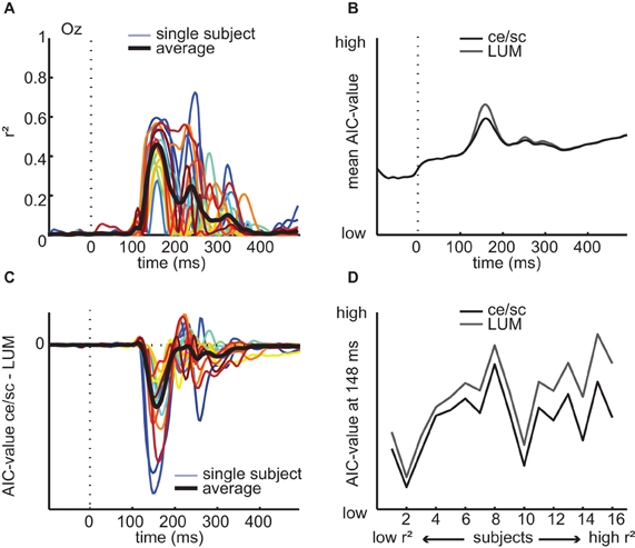
Figure 10. Regression analyses based on LUM values on single-subject ERP data and comparison with contrast statistics. (A) Explained variance at channel Oz for each individual subject (colored lines) and averaged across subjects (black line) from a regression model with LUM values (B) AIC-values of the regression results based on LUM compared to contrast statistics (ce/sc); low AIC-value indicates better model fit. (C) Single-subject differences in AIC-value between LUM and contrast statistics over time. (D) Subject-specific differences in AIC-values at the time-point where the difference between the two models in mean AIC-values is largest (148 ms), sorted based on their maximal r² values of the contrast statistics model. For subjects with higher r² values, the difference in AIC-values becomes somewhat larger, suggesting that high explained variance on contrast statistics is not coupled with increased fit of both models simultaneously, but rather with a better fit of contrast statistics compared to LUM values.

These analyses suggest that despite the high correlations between contrast statistics and simple luminance values, contrast statistics provide a better predictor of perceived invariance as well as differences in evoked activity for this set of texture images. This is not unexpected: from physiology, it is known that neurons in LGN effectively band-pass filter contrast values from the visual input (De Valois and De Valois, 1990). Indeed, repeated band-pass filtering of visual information seems a fundamental property of visual cortex, resulting in increasingly invariant representations (Bouvrie et al., 2009). From this perspective, contrast information is itself more invariant than luminance. Our results suggest that this hierarchical increase in invariance, obtained by filtering, is not equal for all types of textures: after contrast filtering, each image becomes more invariant in information content, but some textures images become more invariant than others, possibly forming a more reliable building block for further processing.

Discussion

In a large database of natural textures, we selected images with low-level contrast statistics that were either constant or variable under changes in illumination angle and orientation. In both EEG and behavior, we showed that textures with little variation in low-level contrast statistics were perceived as more invariant (experiment 1 and 2) and led to more invariant representations at the neural level (experiment 3). The higher the variance in contrast statistics within a given texture, the higher the probability of subjects judging two images of that texture as different categories, specifically if the images differ in illumination direction. Accordingly, high-variant textures give rise to neural evoked responses that are clearly modulated by illumination direction, which is not the case for low-variant textures, as predicted.

Interestingly, as indicated by higher accuracy on same-texture comparisons in the behavioral experiment, textures with low variance in contrast statistics remained more perceptually similar under different illumination (and rotation) conditions. This was explained by the finding that for LV textures, we observed “clustering by texture” of dissimilarities in single-image ERPs between images, whereas there was clustering by illumination direction for HV textures. These results suggest that distance between different textures in terms of contrast statistics—which an observer may use to estimate whether two stimuli are from the same or from a different texture category—are more reliable for LV textures than for HV textures. This is not surprising if one examines the clustering of LV vs. HV stimuli in “contrast statistics space” (Figure 1C): as a natural consequence of the lower variance within LV textures, the differences between texture categories become more similar for images of LV textures.

This work extends recent findings that statistical variations in low-level information are important for understanding generalization over single images (Karklin and Lewicki, 2009). In addition, it has been demonstrated that behavioral categorization accuracy can be predicted using a computational model of visual processing: a neural network consisting of local filters that were first allowed to adapt to the statistics of the natural environment could accurately predict behavioral performance on an object categorization task (Serre et al., 2007). Compared to the latter study, however, in our case there was no training or tuning of a network on a separate set of stimuli such that statistical regularities were implicitly encoded: here, perceived texture similarity was inferred directly from explicitly modeled contrast statistics.

In addition to behavioral categorization, we were able to test the contribution of our two contrast parameters to evoked neural responses using EEG. It is well known that early ERP components can be modulated by low-level properties of (simple) visual input (Luck, 2005). Our finding that contrast energy of single-image responses to natural stimuli is correlated with ERP amplitude around 140–180 ms is also consistent with previous reports of an early time-frame where stimulus-related differences drive evoked responses, e.g., between face stimuli (Philiastides and Sajda, 2006; van Rijsbergen and Schyns, 2009). These authors used classification techniques on single-trial ERPs to show that at later time intervals, differences between individual images correspond to either a more refined representation of the information relevant for the task (van Rijsbergen and Schyns, 2009) or the actual decision made by the subject (Philiastides and Sajda, 2006), suggesting that over the course of the ERP, the visual representation is transformed “away” from simple low-level properties to information that is task-relevant. In this light, it is remarkable that our second image parameter, spatial coherence, is specifically correlated with late ERP activity—around 200 and 300 ms—and that it explains additional variance compared to contrast energy alone specifically in this time interval.

One possible explanation of this apparent discrepancy is that the spatial coherence parameter is itself correlated with more refined or relevant features of natural images: essentially constituting a “summary statistic” of visual input that can be used for rapid decision-making (Oliva and Torralba, 2006). Another interesting hypothesis is that this low-level image parameter is predictive of the availability of diagnostic information, reflecting higher “quality in stimulus information” (Gaspar et al., 2011) or less noise in the stimulus (Bankó et al., 2011; Rousselet et al., 2011), which may influence the accumulation of information for decision-making (Philiastides et al., 2006). Since our two stimulus conditions (HV/LV) were defined based on variance in both contrast energy and spatial coherence, we cannot test which of the two parameters is more strongly correlated with behavioral accuracy. Also, our work is substantially different from these previous reports in that our experiments did not require formation of a high-level representation (e.g., recognition of a face/car), but merely a same-different judgment, essentially constituting a low-level task.

Another difference between our results and those reported in the face processing literature (see e.g., Rousselet et al., 2008) is the localization of our effects. Maximal sensitivity of evoked activity to faces and objects is found at lateral-occipital and parietal electrodes (PO), whereas our correlations, obtained with texture images, are clustered around occipital electrode Oz. This is not unexpected since textural information is thought to be processed in early visual areas such as V2 (Kastner et al., 2000; Scholte et al., 2008; Freeman and Simoncelli, 2011).

In this paper, we specifically aimed to test whether invariance, in addition to a “goal” of visual encoding, could be defined as a property of real-world visual features (in this case, textures). In the first scenario, one would expect the representation of the visual input to change over time to (gradually) become more invariant. Our behavioral results however indicate that variance in low-level properties of natural textures (contrast statistics, presumably derived from very early visual information) can already predict the perceived invariance by human observers under specific viewing manipulations. Moreover, it demonstrates that there are interesting differences between natural textures in terms of this invariance: some textures appear to be surprisingly invariant. It has been argued that, in evolution, mechanisms have evolved for detecting “stable features” in visual input because they are important for object recognition (Chen et al., 2003). In light of the present results, a biologically realistic instantiation of such a stable feature could be “a texture patch whose contrast statistics do not change under viewing variations.” This natural invariance is rooted in physical properties of natural images, but is present at the level of image statistics (stochastic invariance). Such invariance may play an important role in stochastic approaches to computer vision, such as the successful bag-of-words approach (Feifei et al., 2007; Jégou et al., 2011). For example, a patch of a visual scene with more invariant contrast statistics may provide a more reliable “word” for categorization in a bag of words model for scene recognition (Gavves et al., 2011).

Our results suggest that these stochastic invariances are not only reflected in occipital ERPs recorded at the scalp, but that the human visual system may actively exploit them: in the present data, LV textures did not only give rise to more reliable differences between texture categories in evoked responses, but were also associated with more reliable judgments about similarity between different textures—i.e., with behavioral outcome. The link between contrast statistics and categorization accuracy leads to the interesting hypothesis that in more naturalistic tasks such as object detection or natural scene processing, image elements that are stochastically invariant, i.e., reliable, may weigh more heavily in perceptual decision-making than variable, “unreliable” elements.

In sum, the present results show that low-level contrast statistics correlate with variance of natural texture images in terms of evoked responses, as well as perceived perceptual similarity; they suggest that textures with little variance in contrast statistics may give rise to more invariant neural representations. Simply put, invariance in simple, physical contrast information may lead to a more invariant perceptual representation. This makes us wonder about visual invariance as a general real-world property: how much of it can be derived from image statistics? Are there other low-level visual features that differ in their degree of invariance? Next to studying top-down, cognitive invariance, or transformations performed by the visual system to achieve invariance of visual input, exploring to what extent “natural invariances” exist and whether they play a role in visual processing may provide an exciting new avenue in the study of natural scene perception.

Conflict of Interest Statement

The authors declare that the research was conducted in the absence of any commercial or financial relationships that could be construed as a potential conflict of interest.

Acknowledgments

We thank Marissa Bainathsah, Vincent Barneveld, Timmo Heijmans, and Kelly Wols for behavioral data collection of the same-different experiment. This work is part of the Research Priority Program “Brain and Cognition” at the University of Amsterdam and was supported by an Advanced Investigator grant from the European Research Council.

References

Adelson, E. H., and Bergen, J. R. (1991). “The plenoptic function and the elements of early vision,” in Computational Models of Visual Processing, eds M. S. Landy and J. A. Movshon (Cambridge, MA: MIT Press), 3–20.

Akaike, H. (1973). “Information theory and an extension of the maximum likelihood principle,” in Second International Symposium on Information Theory, eds B. N. Petrov and F. Csaki (Budapest: Akademiai Kiado), 267–281.

Bankó, E. M., Gál, V., Körtvélyes, J., Kovács, G., and Vidnyánszky, Z. (2011). Dissociating the effect of noise on sensory processing and overall decision difficulty. J. Neurosci. 31, 2663–2674.

Pubmed Abstract | Pubmed Full Text | CrossRef Full Text

Bergen, J. R., and Julesz, B. (1983). Parallel versus serial processing in rapid pattern discrimination. Nature 303, 696–698.

Pubmed Abstract | Pubmed Full Text

Biederman, I. (1987). Recognition-by-components: a theory of human image understanding. Psychol. Rev. 94, 115–147.

Pubmed Abstract | Pubmed Full Text

Bonin, V., Mante, V., and Carandini, M. (2005). The suppressive field of neurons in lateral geniculate nucleus. J. Neurosci. 25, 10844–10856.

Pubmed Abstract | Pubmed Full Text | CrossRef Full Text

Bouvrie, J., Rosasco, L., and Poggio, T. (2009). On invariance in hierarchical models. Adv. Neural Inf. Process. Syst. 22, 162–170.

Brainard, D. H. (1997). The psychophysics toolbox. Spat. Vis. 10, 433–436.

Pubmed Abstract | Pubmed Full Text | CrossRef Full Text

Chen, L., Zhang, S., and Srinivasan, M. V. (2003). Global perception in small brains: topological pattern recognition in honey bees. Proc. Natl. Acad. Sci. U.S.A. 100, 6884–6889.

Pubmed Abstract | Pubmed Full Text | CrossRef Full Text

Croner, L. J., and Kaplan, E. (1995). Receptive fields of P and M ganglion cells across the primate retina. Vision Res. 35, 7–24.

Pubmed Abstract | Pubmed Full Text | CrossRef Full Text

Daniels, H. E. (1944). The relation between measures of correlation in the universe of sample permutations. Biometrika 33, 129–135.

De Valois, R. L., and De Valois, K. K. (1990). Spatial Vision. New York, NY: Oxford University Press.

DiCarlo, J. J., and Cox, D. D. (2007). Untangling invariant object recognition. Trends Cogn. Sci. 11, 333–341.

Pubmed Abstract | Pubmed Full Text | CrossRef Full Text

Elder, J. H., and Velisavljević, L. (2009). Cue dynamics underlying rapid detection of animals in natural scenes. J. Vis. 9, 1–20.

Pubmed Abstract | Pubmed Full Text | CrossRef Full Text

Elder, J. H., and Zucker, S. W. (1998). Local scale control for edge detection and blur estimation. IEEE Trans. Pattern Anal. Mach. Intell. 20, 699–716.

Feifei, L., Fergus, R., and Perona, P. (2007). Learning generative visual models from few training examples: an incremental Bayesian approach tested on 101 object categories. Comput. Vis. Image Underst. 106, 59–70.

Freeman, J., and Simoncelli, E. P. (2011). Metamers of the ventral stream. Nat. Neurosci. 14, 1195–1200.

Pubmed Abstract | Pubmed Full Text | CrossRef Full Text

Gaspar, C. M., Rousselet, G. A., and Pernet, C. R. (2011). Reliability of ERP and single-trial analyses. Neuroimage 58, 620–629.

Pubmed Abstract | Pubmed Full Text | CrossRef Full Text

Gavves, E., Snoek, C. G. M., and Smeulders, A. W. M. (2011). Visual synonyms for landmark image retrieval. Comput. Vis. Image Underst. 116, 238–249.

Geusebroek, J., and Smeulders, A. W. M. (2002). “A physical explanation for natural image statistics,” in Proceedings of the 2nd International Workshop on Texture Analysis and Synthesis, ed M. Chantler (Edinburgh, Scotland: Heriot-Watt University), 47–52.

Geusebroek, J., and Smeulders, A. W. M. (2005). A six-stimulus theory for stochastic texture. Int. J. Comp. Vis. 62, 7–16.

Ghebreab, S., Smeulders, A. W. M., Scholte, H. S., and Lamme, V. A. F. (2009). A biologically plausible model for rapid natural image identification. Adv. Neural Inf. Process. Syst. 22, 629–637.

Gratton, G., Coles, M. G. H., and Donchin, E. (1983). A new method for off-line removal of ocular artifact. Electroencephalogr. Clin. Neurophysiol. 55, 468–484.

Pubmed Abstract | Pubmed Full Text

Jégou, H., Perronnin, F., Douze, M., Jorge, S., Patrick, P., and Schmid, C. (2011). Aggregating local image descriptors into compact codes. IEEE Trans. Pattern Anal. Mach. Intell. 99. doi: 10.1109/TPAMI.2011.235

Pubmed Abstract | Pubmed Full Text | CrossRef Full Text

Karklin, Y., and Lewicki, M. S. (2009). Emergence of complex cell properties by learning to generalize in natural scenes. Nature 457, 83–86.

Pubmed Abstract | Pubmed Full Text | CrossRef Full Text

Kastner, S., Weerd, P. D., and Ungerleider, L. G. (2000). Texture segregation in the human visual cortex: a functional MRI study. J. Neurophysiol. 2453–2457.

Pubmed Abstract | Pubmed Full Text

Kriegeskorte, N., Mur, M., Ruff, D. A., Kiani, R., Bodurka, J., Esteky, H., Tanaka, K., and Bandettini, P. A. (2008). Matching categorical object representations in inferior temporal cortex of man and monkey. Neuron 60, 1126–1141.

Pubmed Abstract | Pubmed Full Text | CrossRef Full Text

Landy, M. S., and Graham, N. (2004). “Visual perception of texture,” in The Visual Neurosciences, eds L. M. Chalupa and J. S. Werner (Cambridge, MA: MIT Press), 1106–1118.

Li, A., and Zaidi, Q. (2000). Perception of three-dimensional shape from texture is based on patterns of oriented energy. Vision Res. 40, 217–242.

Pubmed Abstract | Pubmed Full Text | CrossRef Full Text

Luck, S. J. (2005). An Introduction to the Event-Related Potential Technique. Cambridge, MA: MIT Press.

Malik, J., and Perona, P. (1990). Preattentive texture discrimination with early vision mechanisms. J. Opt. Soc. Am. A. 7, 923–932.

Pubmed Abstract | Pubmed Full Text

Malik, J., and Rosenholtz, R. (1997). Computing local surface orientation and shape from texture for curved surfaces. Int. J. Comp. Vis. 23, 149–168.

Nothdurft, H. C. (1991). Texture segmentation and pop-out from orientation contrast. Vision Res. 31, 1073–1078.

Pubmed Abstract | Pubmed Full Text | CrossRef Full Text

Nunez, P. L., and Srinivasan, R. (2006). The Neurophysics of EEG, 2nd Edn. Oxford, UK: Oxford University Press.

Pubmed Abstract | Pubmed Full Text | CrossRef Full Text

Oliva, A., and Torralba, A. (2006). Building the gist of a scene: the role of global image features in recognition. Prog. Brain Res. 155, 23–36.

Pubmed Abstract | Pubmed Full Text | CrossRef Full Text

Pelli, D. G. (1997). The VideoToolbox software for visual psychophysics: transforming numbers into movies. Spat. Vis. 437–442.

Pubmed Abstract | Pubmed Full Text | CrossRef Full Text

Perrin, F. (1989). Spherical splines for scalp potential and current density mapping. Electroencephalogr. Clin. Neurophysiol. 72, 184–187.

Pubmed Abstract | Pubmed Full Text

Philiastides, M. G., Ratcliff, R., and Sajda, P. (2006). Neural representation of task difficulty and decision making during perceptual categorization: a timing diagram. J. Neurosci. 26, 8965–8975.

Pubmed Abstract | Pubmed Full Text | CrossRef Full Text

Philiastides, M. G., and Sajda, P. (2006). Temporal characterization of the neural correlates of perceptual decision making in the human brain. Cereb. Cortex 16, 509–518.

Pubmed Abstract | Pubmed Full Text | CrossRef Full Text

Renninger, L. W., and Malik, J. (2004). When is scene identification just texture recognition? Vision Res. 44, 2301–2311.

Pubmed Abstract | Pubmed Full Text | CrossRef Full Text

Riesenhuber, M., and Poggio, T. (1999). Hierarchical models of object recognition in cortex. Nat. Neurosci. 2, 1019–1025.

Pubmed Abstract | Pubmed Full Text | CrossRef Full Text

Rousselet, G. A., Gaspar, C. M., Kacper, P., and Pernet, C. R. (2011). Modeling single-trial ERP reveals modulation of bottom-up face visual processing by top-down task constraints (in some subjects). Front. Psychol. 2:137. doi: 10.3389/fpsyg.2011.00137

Pubmed Abstract | Pubmed Full Text | CrossRef Full Text

Rousselet, G. A., Husk, J. S., Bennett, P. J., and Sekuler, A. B. (2008). Time course and robustness of ERP object and face differences. J. Vis. 8, 1–18.

Pubmed Abstract | Pubmed Full Text | CrossRef Full Text

Scholte, H. S., Ghebreab, S., Waldorp, L., Smeulders, A. W. M., and Lamme, V. A. F. (2009). Brain responses strongly correlate with Weibull image statistics when processing natural images. J. Vis. 9, 1–15.

Pubmed Abstract | Pubmed Full Text | CrossRef Full Text

Scholte, H. S., Jolij, J., Fahrenfort, J. J., and Lamme, V. A. (2008). Feedforward and recurrent processing in scene segmentation: electroencephalography and functional magnetic resonance imaging. J. Cogn. Neurosci. 20, 2097–2109.

Pubmed Abstract | Pubmed Full Text | CrossRef Full Text

Serre, T., Oliva, A., and Poggio, T. (2007). A feedforward architecture accounts for rapid categorization. Proc. Natl. Acad. Sci. U.S.A. 104, 6424–6429.

Pubmed Abstract | Pubmed Full Text | CrossRef Full Text

van Rijsbergen, N. J., and Schyns, P. G. (2009). Dynamics of trimming the content of face representations for categorization in the brain. PLoS Comp. Biol. 5:e1000561. doi: 10.1371/journal.pcbi.1000561

CrossRef Full Text