Modeling and simulation of multi-scale environmental systems with Generalized Hybrid Petri Nets

Introduction

The process of constructing and analyzing environmental systems is increasingly becoming a complex procedure (Seppelt et al., 2009; Uusitalo et al., 2015). On the one hand, it can require the amalgamation of different simulation techniques to accurately and efficiently find a solution to the problem under consideration (see e.g., Gillet, 2008; Gregorio et al., 1999). On the other hand, complex environmental systems require the collection and analysis of various data and information that cannot be tackled by researchers coming from just one area of expertise (Seppelt et al., 2009).

While the ordinary differential equations (ODEs) approach is widely used to construct and simulate many problems in the environmental domain, certain classes of such problems cannot be adequately addressed using this approach alone. For instance in Khoury et al. (2013) construct a simple, but elegant ODEs model to study food and population dynamics in honey bee colonies. However, such a continuous approach cannot capture the effect of seasonal variations on many parameters. Contrary, in Schmickl and Crailsheim (2007) and Russell et al. (2013) a discrete simulation of recurrence and difference equations has been deployed to emulate the discrete changes in bee population taking into account seasonal variations. Nevertheless, certain scenarios necessitate the interplay of different simulation strategies to efficiently and accurately simulate a given problem. For example, the ODE approach can be used to efficiently execute model components with fast dynamics where elucidated discrete simulation does not affect the result, while stochastic simulation has to be used to discretely model components whose individual and random occurrence plays a key role for the overall result. Such type of models possess more than one time scale. Therefore, it requires hybrid simulation to successfully reproduce their dynamics. This results in two or more simulation regimes which have to work simultaneously to solve a given problem. However, these regimes are not isolated, instead, they closely interact and influence the dynamics of each other (Herajy and Heiner, 2012).

Furthermore, with the increasing demand for interdisciplinary science, modeling complex environmental systems may involve researchers with different scientific and educational background. For instance, researchers from ecosystems, mathematics, and computer science may collaborate in constructing and analyzing a computational experiment. Nonetheless, maintaining the communication in such interdisciplinary teams is one of the key issues in constructing environmental models (Seppelt et al., 2009). Thus, a visual language may be of help to accelerate the communication between team members with diverse professional background. As an example, consider the problem of water resource management. Numerical modeling and simulation play a remarkable role in predicting future water demand as well as managing water quality (Qi and Chang, 2011; Liu et al., 2015). However, the procedure of constructing a realistic and accurate model for this purpose mandates that a team of experts coming from different fields (e.g., environmental science, mathematics, geography, hydrological modeling, and computer science) collaborate closely together.

One of those modeling tools that can contribute in overcoming these challenges are Petri nets. Petri nets (Murata, 1989) are a visual modeling language highly suitable to model concurrent, asynchronous and distributed systems. In addition to their graphical representation, Petri nets enjoy a well established mathematical theory to analyze the constructed model. However, the basic place/transition nets are not very helpful in constructing and executing quantitative models exposing certain level of complexities. Therefore, many extensions have been proposed over the years to overcome these limitations. For instance, continuous Petri nets (Alla and David, 1998) can be used as an alternative technique which exactly corresponds to the ODEs approach (Gilbert and Heiner, 2006; Soliman and Heiner, 2010). Similarly, stochastic Petri nets (Ajmone et al., 1995) provide a graphical tool to permit the stochastic exploration of a constructed model. Nowadays, a variety of Petri nets with different extensions have been used to model various technical and biological systems (e.g., see Reddy et al., 1993; Matsuno et al., 2003; Fujita et al., 2004; Herajy et al., 2013).

Hybrid Petri Nets () (David and Alla, 2010) are another interesting class of Petri nets. permit the integration of discrete and continuous variables (places) in addition to discrete and continuous processes (transitions) into one model. In a typical scenario, discrete places serve as signals that control the firing of continuous transitions. allow the efficient simulation of systems which entail large number of states by approximating them via continuous simulation, while discrete events can be pertained using discrete transitions. In Matsuno et al. (2003), are adapted to provide a very specific approach dedicated to the simulation of biological systems. In general, hybrid modeling using is a promising technique since it permits the simulation of more complex systems (see e.g., Tian et al., 2013). Furthermore, models with interacting components working at different scales can be easily executed via . Nevertheless, so far, little attention has been paid to the employment of this approach in the context of modeling environmental systems.

In this paper, we focus on a particular class of hybrid Petri nets, Generalized Hybrid Petri nets () (Herajy and Heiner, 2012), as a promising tool for model-based exploration of environmental systems. provide various transitions, arcs, and places, which together have the power to substantially facilitate the modeling of different processes in the environmental science. One important aspect of is their ability to simulate systems that expose different time scales: fast and slow. The former time scale is continuously simulated, while the latter one is stochastically and individually executed. Furthermore, the interaction between continuous and stochastic dynamics is appropriately captured. We illustrate the use of in modeling environmental systems via a case study, the Chagas disease infection cycle. All the discussed features in this paper are implemented in a general platform-independent Petri net editing tool called Snoopy (Heiner et al., 2012) which can be downloaded free of charge for academic use from Snoopy (2015).

The rest of this paper is organized as follows: after this introduction, the different aspects of are discussed by presenting a formal definition as well as the different modeling elements of . Afterwards, the main steps involved in the simulation of are briefly summarized. In the Result section, we provide a case study to illustrate the use of for modeling environmental systems, namely the simulation of infection transmission of Chagas disease. This example explains the motivation behind most of the modeling components. Finally, we conclude with a few remarks concerning the utilization of to implement the simulation of multi-scale environmental models.

Methods

In this section we provide an overview of including the formal definition as well as their different modeling elements. We concentrate in this part on the use of for the modeling of environmental systems. Thus, the semantics of places, transitions and arcs are discussed according to this context.

Generalized Hybrid Petri Nets

Elements

As a Petri net class, the specification of involves defining the three main components, namely: places, transitions, and arcs. Figure 1 illustrates the different entities that can be found in a typical model. In the sequel, we briefly discuss the semantics and usage of each constituent.

FIGURE 1

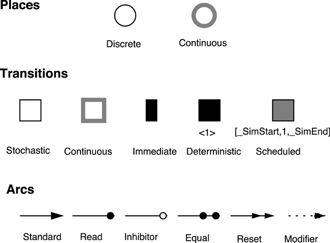
Figure 1. Graphical representation of the elements (Herajy and Heiner, 2012). Places are classified as discrete and continuous; transitions as continuous, stochastic, immediate, deterministically delayed and scheduled; and arcs as standard, inhibitor, read, equal, reset, and modifier.

Places

Places correspond to the model variables. They are further classified into discrete and continuous. On the one hand, discrete places are drawn as single line circles. They are used to represent discrete variables (e.g., the number of trees in a forest, the number of eggs laid by a bee, or a species population). Discrete places can hold nonnegative integer numbers called tokens. On the other hand, continuous places are drawn with shaded line circles and are used to depict continuous variables (e.g., the amount of water in a lake, the concentration of contaminated water, or the number of infected individuals in an epidemic model). Therefore, they can hold nonnegative real values. In certain modeling scenarios, continuous places serve as an approximation of discrete places where the numbers of tokens reach large values. The value assigned to a place is called place marking. In models, the system state is described at any time point during the simulation as the union of discrete and continuous place marking.

Transitions

Transitions correspond to the basic events. employ five transition types for convenient modeling of different types of systems: stochastic, immediate, deterministically time delayed, scheduled, and continuous transitions. The first four transition types are discrete ones. However, they differ from each other by the time delay assigned to them.

Stochastic transitions fire at discrete time steps, however, after random time delays. These random delays are exponentially distributed. Stochastic transitions can represent events that take place at random time steps. During execution, the simulator calculates the time at which the next event will occur, and subsequently it decides the event type (which transition to fire). Theoretically, an effective conflict (David and Alla, 2010) between two stochastic transitions is not possible in a such random firing scheme. Immediate transitions are also fired in a discrete manner, but with zero delays. They fire directly as soon as they are enabled. Similarly, deterministically time delayed transitions are fired after a deterministic time delay. The delay of this transition type could be set to zero. Nevertheless, when an immediate transition and a deterministically delayed transition are concurrently enabled, the immediate one will have higher priority to fire first. Moreover, scheduled transitions are a special type of deterministically time delayed transitions which fire at certain time point(s) previously programmed by the user.

In contrast, continuous transitions fire continuously with respect to time. The firing speeds of continuous transitions are specified by their rates. Besides, the semantics of continuous transitions is represented by a set of ODEs that account for in- and outflow of each place.

Arcs

Arcs model the relation between the model variables and the basic events. Arcs connect places with transitions and maybe vice versa depending on their type. There are six type of arcs in : standard, read, inhibitor, equal, reset, and modifier arcs.

Standard arcs connect places with transitions and vice versa. They control the enabling of the target transition as well as affecting the preplaces (postplaces) when the target (source) transition fires. Standard arcs can be discrete or continuous. Discrete arcs adopt positive integer values as arc weights, while continuous arcs use positive rational numbers as arc weights. The rules that determine the type of arc weights are illustrated in Figure 2.

FIGURE 2

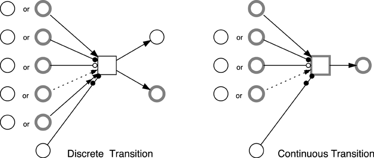
Figure 2. Possible connections between elements. The (obvious) restrictions are: discrete places cannot be connected with continuous transitions using standard arcs, continuous places cannot be tested with equal arcs, and continuous transitions cannot use reset arcs.

In contrast, read arcs affect only the enabling of the target transition. A transition connected with a preplace via a read arc is enabled only (with respect to this preplace), if the marking of this preplace is greater than or equal to the corresponding arc weight. Similarly, inhibitor arcs govern the enabling of transitions. However, a transition connected with a preplace using an inhibitor arc is enabled only if the current marking of the preplace is less than the arc weight. Equal arcs enforce more stronger conditions on the enabling of transitions. A transition connected with a preplace via an equal arc is enabled only if the current marking of the preplace is exactly equal to the arc weight.

The other two remaining arcs do not influence the enabling of the connected transitions. For example, reset arcs set the value of the preplace marking to zero when the corresponding transition fires. They are useful to implement certain model semantics. Similarly, modifier arcs do not affect the enabling nor the firing of a transition. They facilitate the use of a preplace in defining a transition rate function while preserving the structure-related constraints of the transitions' rate functions.

Marking-dependent Arc Weights

permit arc weights to be specified as an algebraic expression involving place names rather than just a constant. This feature is called marking-dependent arc weights (Valk, 1978; Matsuno et al., 2003; Herajy et al., 2013). Implementing certain model semantics without the help of marking-dependent arc weights may become intricate and even impossible in certain circumstances.

For instance, consider the following model expression that requires to be implemented using Petri nets:

IF x>=y AND y<5 THEN
  
     z:=x+y
  
END IF

When x, y, and z are continuous variables, it is impossible to represent the above semantics using just arcs with constant weights. However, using marking-dependent arc weights this can be easily modeled as it is depicted in Figure 3.

FIGURE 3

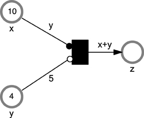
Figure 3. A example of using marking-dependent arc weights. The example contains three places x, y, z and one immediate transition t₁. The transition t₁ can fire only when the two conditions: x≥y (enforced by the read arc) and y < 5 (enforced by the inhibitor arc) hold.

As another interesting example of the usefulness of marking-dependent arcs consider the transformation of the whole population from one age category to another one after an elapsed period of time. For example in Xiang et al. (2013), new-born snails are considered as old snails at the beginning of the year. This process can be intuitively modeled using marking-dependent arc weights where the outgoing and the ingoing arc weights equal the value of the preplace.

Obviously, marking-dependent arc weights extend and permit the modeling of a larger class of environmental systems that require the corresponding semantics.

Formal Definition

In this section we formally define the syntax of . The formal semantics including the enabling and firing rules as well as the conflict resolution are given in Herajy and Heiner (2012).

Definition 1 (Generalized Hybrid Petri Nets). Generalized Hybrid Petri Nets are a 6-tuple = [P, T, A, F, V, m₀], where P, T are finite, non-empty and disjoint sets. P is the set of places, and T is the set of transitions with:

• P = P_disc ∪ P_cont whereby P_disc is the set of discrete places to which non-negative integer values are assigned, and P_cont is the set of continuous places to which non-negative real values are assigned.

• T = T_D ∪ T_cont,

T_D = T_stoch ∪ T_im ∪ T_timed ∪ T_scheduled with:

1. T_stoch is the set of stochastic transitions, which fire randomly after exponentially distributed waiting time.

2. T_im is the set of immediate transitions, which fire with waiting time zero; they have highest priority among all transitions.

3. T_timed is the set of deterministically delayed transitions, which fire after a deterministic time delay.

4. T_scheduled is the set of scheduled transitions, which fire at predefined time points.

5. T_cont is the set of continuous transitions, which fire continuously over time.

• A = A_disc ∪ A_cont ∪ A_inhibit ∪ A_read ∪ A_equal ∪ A_reset ∪ A_modifier is the set of directed arcs, with:

1. A_disc ⊆ ((P × T) ∪ (T × P)) defines the set of discrete arcs.

2. A_cont ⊆ ((P_cont × T) ∪ (T × P_cont)) defines the set of continuous arcs.

3. A_read ⊆ (P × T) defines the set of read arcs.

4. A_inhibit ⊆ (P × T) defines the set of inhibits arcs.

5. A_equal ⊆ (P_disc × T) defines the set of equal arcs.

6. A_reset ⊆ (P × T_D) defines the set of reset arcs,

7. A_modifier ⊆ (P × T) defines the set of modifier arcs.

•. the function F

$F:\{\begin{array}{l}{A}_{cont}\to D_q,\hfill \\ A_{disc}\to D_n,\hfill \\ A_{read}\to D_q,\hfill \\ A_{inhibit}\to D_q,\hfill \\ A_{equal}\to D_n,\hfill \\ A_{reset}\to \left\{1\right\},\hfill \\ A_{modifier}\to \left\{1\right\}.\hfill \end{array}$

assigns a marking-dependent function to each arc, where D_n and D_q are sets of functions defined as follows:

$D_n=\{d_n|d_n:{\mathbb{N}}_0^{|\bullet t_j|}\to \mathbb{N},t_j\in T\},$

$D_q=\{d_q|d_q:{ℝ}_0^{|\bullet t_j|}\to {\mathbb{Q}}^{+},t_j\in T\}.$

• V is a set of functions V = {g, d, w, f} where :

1. g : T_stoch → H_s is a function which assigns a stochastic hazard function h_st to each transition t_j ∈ T_stoch, whereby $H_s=\{h_{s_t}|h_{s_t}:{ℝ}_0^{{|}^{\bullet }{t}_j|}\to {ℝ}_0^{+},t_j\in T_{stoch}\}$ is the set of all stochastic hazard functions, and g(t_j) = h_st, ∀t_j ∈ T_stoch.

2. w : T_im → H_w is a function which assigns a weight function h_w to each immediate transition t_j ∈ T_im, such that $H_w=\{h_{w_t}|h_{w_t}:{ℝ}_0^{{|}^{\bullet }{t}_j|}\to {ℝ}_0^{+},t_j\in T_{im}\}$ is the set of all weight functions, and w(t_j) = h_wt, ∀t_j ∈ T_im.

3. $d:T_{timed}\cup T_{scheduled}\to {ℝ}_0^{+}$, is a function which assigns a constant time to each deterministically delayed and scheduled transition representing the (relative or absolute) waiting time.

4. f : T_cont → H_c is a function which assigns a rate function h_c to each continuous transition t_j ∈ T_cont, such that $H_c=\{h_{c_t}|h_{c_t}:{ℝ}_0^{{|}^{\bullet }{t}_j|}\to {ℝ}_0^{+},t_j\in T_{cont}\}$ is the set of all rates functions and f(t_j) = h_ct, ∀t_j ∈ T_cont.

• m₀ = m_disc ∪ m_cont is the initial marking for both the continuous and discrete places, whereby $m_{cont}\in {ℝ}_0^{|P_{cont}|}$, $m_{disc}\in {\mathbb{N}}_0^{|P_{disc}|}$.

Here, ℕ₀ denotes the set of non-negative integer numbers, ℝ₀ denotes the set of non-negative real numbers, ℚ⁺ denotes the set of positive rational numbers, and ^•t_j denotes the set of pre-places of a transition t_j.                            □

A distinguishing feature of compared with other hybrid Petri net classes is its support of the full interplay between stochastic and continuous transitions. Such interplay is implemented by updating and monitoring the rates of stochastic transitions The crucial point for our paper is how stochastic transitions are simulated when mixed with continuous ones. So the next section focuses in particular on the simulation of stochastic transitions, while numerically solving the set of ODEs induced by the continuous transitions (for more details see Herajy and Heiner, 2012). By this way, accurate results are obtained during simulation.

Simulation

The simulation of a model has to take into account the different types of transitions. Although it is easy to simulate individual transition types when they are isolated, it becomes more challenging to simulate a model combining discrete and continuous transitions. Thus, the most important aspect is how discrete and continuous transitions are interleaved during the simulation, particularly, stochastic and continuous ones.

Continuous transitions are fired continuously. Thus, they necessitate the simultaneous (numerical) solution of a system of ODEs representing the continuous part of a model. From this perspective, the simulation of discrete transitions are considered as events which are triggered whenever a discrete transition is enabled and needs to be fired. Therefore, we have different events corresponding to each transition type. When an event occurs, a dispatcher is called to handle the appropriate actions. The corresponding system of ODEs is generated using (1).

$\begin{array}{cc}\begin{array}{l}\frac{dm\left(p_i\right)}{d\tau }={\displaystyle \sum _{t_j{\in }^{•}{p}_i}F}\left(t_j,p_i\right)·v_j\left(\tau \right)·read(u,m(p_i))·inhibit(u,m(p_i))-\\ {\displaystyle \sum _{t_j\in p_i{}^{•}}F}\left(p_i,t_j\right)·v_j\left(\tau \right)·read(u,m(p_i))·inhibit(u,m(p_i))\end{array}& (1)\end{array}$

where m(p_i) represents the marking of the place p_i, v_j(τ) = f_j is the marking-dependent rate function of the continuous transition t_j, and the functions read(u, p_i), inhibit(u, p_i), which consider the effects of read and inhibitor arcs, respectively, are defined as follows:

For a given transition t_j ∈ T^C,

$read(u,m(p_i))=\{\begin{array}{ll}1\hfill & \text{if }m(p_i)\ge u\hfill \\ 0\hfill & \text{else}\hfill \end{array}$

with u = F(p_i, t_j) ∧ (p_i, t_j) ∈ A_read, and

$inhibit(u,m(p_i))=\{\begin{array}{ll}1\hfill & \text{if }m(p_i)<u\hfill \\ 0\hfill & \text{else}\hfill \end{array}$

with u = F(p_i, t_j) ∧ (p_i, t_j) ∈ A_inhibit.

Furthermore, two issues are of paramount importance concerning this simulation procedure: how an event is detected during the numerical solution of the set of ODEs and how we know that a stochastic transition is enabled and needs to be fired.

Concerning the former issue, a special type of ODE solver should be used that supports a root finding feature (Mao and Petzold, 2002). The occurrence of enabling conditions of discrete transitions are then formulated as a root that can be detected by the ODE solver. As soon as a root is encountered by the ODE solver, the control is transferred to the discrete regime to fire the enabled transition(s). Afterwards, the ODE solver continues the integration using the new system state.

Moreover, stochastic transitions are considered as a special type of discrete events called stochastic events. Stochastic events are detected by introducing a new ODE, described by Equation (2), to the set of ODEs.

$\begin{array}{cc}g(x)={\displaystyle {\int }_t^{t+\tau }{a}_0^s(x)dt}-\xi =0,& (2)\end{array}$

where ξ is a random number exponentially distributed with a unit mean, and a^s₀(x) is the cumulative (the sum) rate of all stochastic transitions.

The newly added ODE monitors the difference between the summation of all the rates of the stochastic transitions and a small, exponentially distributed random number. When Equation (2) equals zero, the continuous simulation is interrupted to call the dispatcher to fire the enabled stochastic transition. Afterwards, the simulation is resumed as previously discussed.

Results

In this section we apply to model and simulate a case study from the environmental domain. can be used for models which are completely deterministic, completely stochastic, or a combination of them. The chosen example illustrates the use of to represent and simulate the dynamics of environmental and ecological systems. We show how stochastic and continuous transitions are used to provide the interplay between a discrete regime representing the environment fluctuations and a deterministic one representing the simulation of large populations. Additionally, deterministically time delayed transitions and immediate transitions proved to be useful in modeling real-life examples.

Modeling the Transmission of Chagas Disease Infection

Background

The Chagas disease has been a major public health concern in Latin America for some decades (Nouvellet et al., 2015). The transmission of Chagas infection among humans involves complex ecological and epidemiological interacting processes (Cohen and Gürtler, 2001; Nouvellet et al., 2015). The Chagas disease is caused by the protozoan Trypanosoma Cruzi (T. Cruzi for short). The main insect vector responsible for the transmission of T. Cruzi is a bug known as Triatoma infestans (Cohen and Gürtler, 2001; Castañera et al., 2003). A vector is an insect that transmits a disease, while the disease transmitted via such an insect is referred to as a vector-borne disease. Vectors are living organisms that can transmit infectious diseases between humans or from animals to humans. Many of these vectors are bloodsucking insects. Within a household, Chagas disease is mainly transmitted to humans via the bitting by infected bugs (Castañera et al., 2003). Bugs acquire infections by the feeding on infected mammals (humans or dogs) (Cohen and Gürtler, 2001). Chickens are another feeding source for Triatoma infestans. However, blood meals taken from chickens do not transmit the infection to bugs. Therefore, chickens can serve as an alternative feeding source to Triatoma infestans such that bitting rates of vectors to humans and infected dogs are minimized (Cohen and Gürtler, 2001). Nevertheless, the four species involved in the Chagas disease cycle are: humans, dogs, chickens, and infected vectors. Besides, the population of Triatoma infestans is oscillating seasonally with the highest population of vectors recorded in warm seasons (spring and summer) (Cohen and Gürtler, 2001).

Mathematical modeling of the transmission of the Chagas disease is an important tool to understand the biological and ecological factors influencing the spread of infections among humans and household animals. To this end, many mathematical models have been constructed (see e.g., Cohen and Gürtler, 2001; Castañera et al., 2003; Coffield et al., 2013; Nouvellet et al., 2015). However, all of these models utilize solely either the deterministic or the stochastic approach. For the former modeling paradigm, authors argue that the population size of the interacting species is large enough so that the ODE approach can be deployed to study the model dynamics (Coffield et al., 2013). In contrast, the latter models assume that the population size of interacting species is relatively small. Thus, stochastic simulation will be more accurate (Castañera et al., 2003). For instance, in Cohen and Gürtler (2001) the number of humans of a household consists of just five persons divided into different age categories. Each category contains only one human. Nevertheless, modeling the transmission of the Chagas disease can encompass variables interacting at different time scales. For instance, vertebrate species (humans, dogs, and chickens) can be found in scales of tens or hundreds at the very most, because the majority of realistic models operate on the level of small villages. In contrast, vector population is abundant and exists at the scale of thousands. Thus, hybrid modeling is a desirable approach worth being investigated to gain deeper understanding of the Chagas disease transmission.

Model Specification

In this section we use to model the transmission of Chagas infection between humans, dogs, and vectors. Our model is based on the deterministic one by Coffield et al. (2013) as it accounts for the high-level transmission of infections without considering the detailed stages of nymph bugs.

Coffield et al. (2013) simulated the evolution of the total population of vectors, humans, and dogs involved in the transmission of Chagas disease. The chicken population is considered to be constant. Their population change is not taken into account since they do not acquire infection. Figure 4 provides a representation of the Chagas transmission cycle. To simplify the discussion, we divide the human population into two groups: infected (denoted by the place H_i), and susceptible (denoted by the place H_s). Similarly, we divide the population of dogs into infected dogs (D_i), and susceptible ones (D_s). In contrast, we consider the total population of vectors (V) and the infected ones (V_i) to minimize the connection among the model components. We adopt the concept of logical places (places represented in gray colors) to keep the connection between model components intelligible. Moreover, the current simulation time (in days) is represented by the discrete place: time. The deterministically time delayed transition increase_days increases the simulation time by a one-day step. The value of the place time is reset after a duration of 365 days. Read and reset arcs as well as the immediate transition reset_days implement the reset semantics of the current year as it can be seen in Figure 4. Furthermore, continuous and stochastic transitions model the dynamics of the different processes involved in the Chagas disease infection cycle.

FIGURE 4

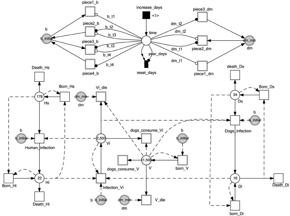
Figure 4. model of Chagas disease transmission. Continuous and discrete places are used to model the population of vectors and mammals, while continuous transitions are adopted to represent the processes operating on the model species. The simulation time is monitored by the discrete place time which is increased by one time step (one day) when the deterministically delayed transition increase_days fires. Stochastic and continuous transitions describe physical processes that operate on the model species. Places given in gray are logical places which help to simplify the connections between model components. Please note the use of modifier arcs to include non-preplaces into the transition rate functions. Modifier arcs make this kind of dependency explicit. Moreover, arc weights and initial markings specified by constants make the model easy to configure using different constant values.

In the sequel we elucidate the definition of each transition rate. Moreover, we discuss our motivation of modeling certain processes as stochastic transitions and others as continuous ones by showing the effect of the random firing of stochastic transitions on the overall dynamic results. Similar to Coffield et al. (2013), we consider the total population of humans, dogs, and chickens as being constant during the whole simulation period. The total human population is considered to be roughly constant as the sum of the number of infected humans and the number of susceptible humans does basically not change, if we assume equal rates for birth and death. Likewise, the dog population is also considered to be constant. However, the number of chickens are not divided into infected and susceptible, since chickens cannot be infected. More information is provided in the equations below.

First, the growth of the total vector population is defined by Equation (3) (Coffield et al., 2013).

$\begin{array}{ll}{d}_h\times (V)\times (1-\frac{V}{K})& (3)\end{array}$

Where d_h is the vector hatching rate, and K specifies the maximum number of bugs that can be supported in a village. Equation (3) is used to define the rate of the transition born_V. The hatching rate coefficient d_h is defined in terms of the biting rates b, which is varying seasonally (see below). Please note that we assume that the rate at which vectors hatch at time t is equal to the number of eggs laid at time t+τ.

Furthermore, vectors undergo two types of death: degradation due to natural death and by the oral consumption by dogs (Coffield et al., 2013). These two processes are represented by the two transitions: dogs_consume_V, and V_die, respectively. The rates of the transitions dogs_consume_V, and V_die are defined by Equations (4) and (5), respectively.

$\begin{array}{rc}\left(\frac{E\times V}{V+A}\right)\times D& (4)\end{array}$

$\begin{array}{rc}\left(\frac{d_m}{2}\times \left(1-\frac{V}{K}\right)+d_m\right)\times V& (5)\end{array}$

where E is the maximum number of vectors consumed by one dog per day, A is the vector number at which dogs consume at the rate E/2 vectors per day, and d_m is the mortality rate coefficient.

The mortality rate coefficient of infected and uninfected vectors is not constant. Instead, it is changing with respect to time according to the current season (Castañera et al., 2003; Coffield et al., 2013). Figure 5 illustrates the time-dependent mortality rate of Triatoma infestants, while Figure 6 is a Petri net sub model used to reproduce the piecewise function in Figure 5. To model the seasonal variation in mortality rate, we adopt read and inhibitor arcs to define the time period of each piece of the piecewise function. The current value of the mortality rate is represented by the continuous place d_m. Two constant values, dm_initial, dm_max are used to denote the initial and maximum values of dm, respectively. The x-axis of the piecewise function in Figure 5 is divided into three intervals [0, dm_t₁[, [dm_t₁, dm_t₂[, and [dm_t₂, year_days]. Where year_days denotes the number of days per year (in our model we consider each year to consist of 365 days). Read arcs are used to specify the interval's lower value, while inhibitor arcs are used to specify the interval's upper values. Afterwards, each continuous transition piece1_dm, piece2_dm, and piece3_dm get assigned the rates, (dm_max−dm_initial)/dm_t₁, dm_max/(dm_t₂ − dm_t₁), and dm_inial/(year_days−dm_t₂), respectively. For the simulation results in this paper we assign the values 0.0003, 0.0017,136, 228, and 365 to dm_initial, dm_max, dm_t₁, dm_t₂, and year_days respectively. A similar procedure is applied to capture the seasonal variation in the biting rate, as it can be noted in Figures 5, 6. The complete list of all constant values is provided in the Supplementary Table 1.

FIGURE 5

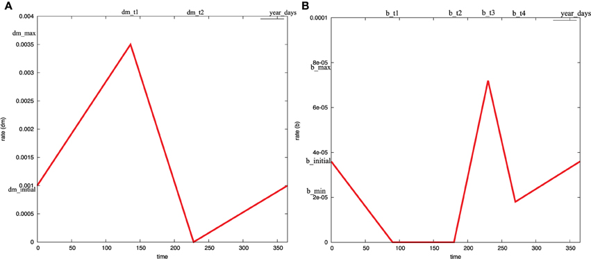
Figure 5. The effects of seasonal variability on: (A) the mortality rate coefficient, and (B) the biting rate coefficient. These curves can be modeled as piecewise linear functions (Coffield et al., 2013). They can be produced using the Petri net submodel in Figure 6. The time boundaries where the functions change their behavior from decreasing to increasing or vice versa is shown in the x-axis. The exact time points where the functions change their behavior is illustrated in the upper axis. Similarly, the start and end values of each piece is shown in the y-axis. The exact values of these parameters are given in the Supplementary Material.

FIGURE 6

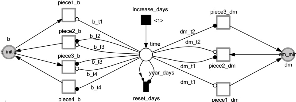
Figure 6. submodel to reproduce the seasonal variability on mortality and biting rates. The deterministically time delayed transition, increase_days, fires at each time step increasing the current simulation time by one day. The immediate transition reset_days resets the current time to zero when it reaches the maximal number of days in a year. Continuous transitions are used to simulate the various pieces of the piecewise linear functions describing the mortality and biting rates. All labels at arcs or places are constants; compare caption of Figure 4.

Similarly, the infected vector population can grow, naturally die, or be consumed by dogs. The increase of infected bugs is a result of the transmission of T. Cruzi parasites to some of the uninfected vectors. In our model, this process is represented by the transition Infection_V_i with a firing rate defined by Equation (6).

$\begin{array}{ll}b\times (V-V_i)\times (P_{hv}\times H_i+P_{dv}\times d_f\times D_i)& (6)\end{array}$

where P_hv is the human to vector infection probability, P_dv is the dogs to vector infection probability, and d_f is the human factor of one dog.

Moreover, the natural death of vectors and the loss of vectors due to the consumption by dogs are modeled by the two transitions: Vi_die and dogs_consume_V_i, respectively. The rate of Vi_die is defined by Equation (7), similar to the death of the total vectors V, while the rate of dogs_consume_Vi is defined by Equation (8).

$\begin{array}{ll}\left(\frac{d_m}{2}\times \left(1-\frac{V}{K}\right)+d_m\right)\times V_i& (7)\end{array}$

$\begin{array}{ll}\frac{E\times D\times V_i}{V+A}& (8)\end{array}$

Now we consider the dynamics of humans and dogs. Susceptible humans (H_s) can be bitten by vectors and become infected (H_i). The infection process is denoted by the transition Human_infection. The firing rate of this transition is given by Equation (9)

$\begin{array}{ll}b\times P_{vh}\times H_s\times V_i& (9)\end{array}$

where P_vh is the probability of a susceptible human to be infected. A human infected by Chagas disease unfortunately cannot be recovered in the future. Both susceptible and infected humans can die with rates defined by Equations (10) and (11), respectively.

$\begin{array}{ll}{\gamma }_{H_s}\times H_s& (10)\end{array}$

$\begin{array}{ll}{\gamma }_{H_i}\times H_i& (11)\end{array}$

where γ_Hs, and γ_Hi are the mortality rates of susceptible and infected humans, respectively. Equations (10) and (11) define the rates of the transitions: death_Hs, and death_Hi, respectively.

Under the assumption that the number of humans are constant during the whole simulation period, the growth rate of susceptible and infected humans can be made equal to their corresponding death rate. However, according to Coffield et al. (2013), infection can be transferred from a mother to her fetus. Thus, we can model the growth of susceptible and infected human using Equations (12) and (13), respectively,

$\begin{array}{ll}(1-T_{hi})\times ({\gamma }_{H_i}\times H_i+{\gamma }_{H_s}\times H_s)& (12)\end{array}$

$\begin{array}{ll}(T_{hi})\times ({\gamma }_{H_i}\times H_i+{\gamma }_{H_s}\times H_s)& (13)\end{array}$

where T_ni is the congenital transmission probability for infected humans. Equations (12) and (13) imply that we take T_ni, the total of died humans (infected and susceptible) as new born infected humans, while the remaining 1 − T_ni are added to the suspected humans.

Likewise, susceptible dogs can be infected with T. Cruzi parasites. However, an infection is transmitted to dogs either by the bitting by vectors or by the oral consumption of infected vectors by dogs. This process is modeled by the transition dogs_infection in Figure 4. The transition rate is given by Equation (14).

$\begin{array}{ll}b\times d_f\times P_{vdb}+\frac{P_{vdc}\times E\times D_s\times V_i}{V+A}& (14)\end{array}$

where P_vdb denotes the vector to dog infection probability, and P_vdc the vector to dog infection probability via oral consumption. Obviously, the first term of Equation (14) represents the dogs infection via bug biting while the second term represents dog infection via oral consumption. Similar to humans, dogs (susceptible and infected) may die. The death of susceptible and infected dogs is represented by the transitions death_Ds, and born_Di, respectively. The firing rates of these transitions are given by Equations (15) and (16), respectively.

$\begin{array}{ll}{\gamma }_{D_s}\times D_s& (15)\end{array}$

$\begin{array}{ll}{\gamma }_{D_i}\times D_i& (16)\end{array}$

Similar to humans, and under the assumption that the overall dog population is constant during the whole simulation period, we set the rate of growth equal to the rate of death. However, new born dogs can be infected if they are born to an infected mother. Thus, the growth rates of susceptible and infected dogs are defined by Equations (17) and (18), respectively.

$\begin{array}{ll}(1-T_{di})\times ({\gamma }_{Di}\times D_i+{\gamma }_{D_s}\times D_s)& (17)\end{array}$

$\begin{array}{ll}(T_{di})\times ({\gamma }_{Di}\times D_i+{\gamma }_{D_s}\times D_s)& (18)\end{array}$

where T_di is the congenital transmission probability for infected dogs. The complete model definition is provided in Figure 4, while the meaning and rate function of each transition are summarized in the Tables 1, 2.

TABLE 1

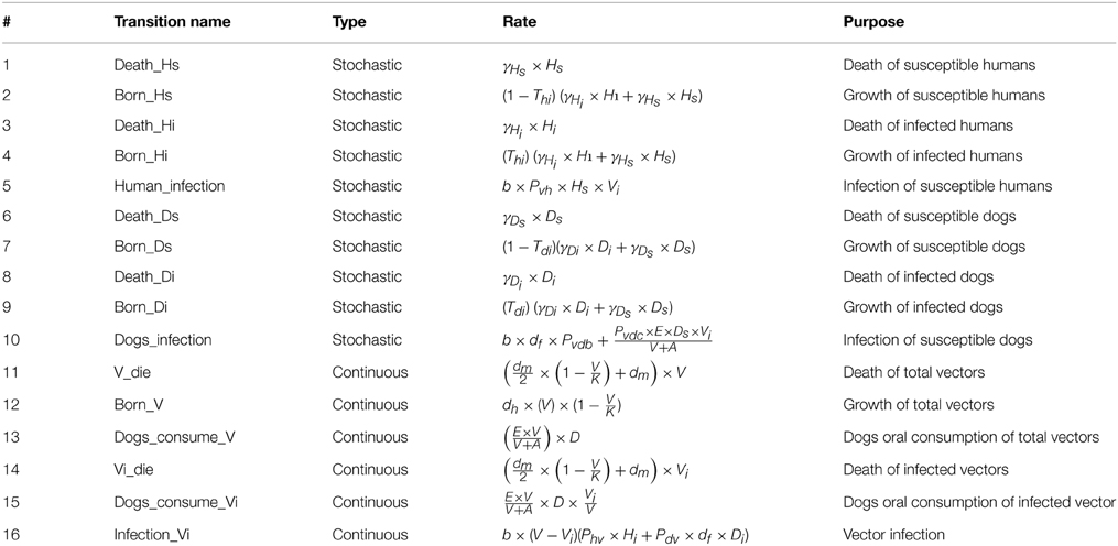
Table 1. Detailed specification of the main transitions of the model in Figure 4.

TABLE 2

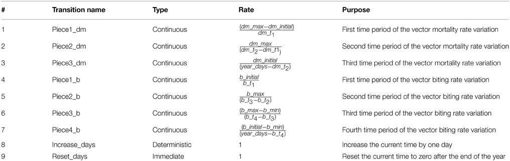
Table 2. The specification of the transitions involved in mortality and the biting rate of the submodel in Figure 6.

Model Simulation

The model in Figure 4 is executed using Snoopy's hybrid simulation engine (Herajy and Heiner, 2012; Heiner et al., 2012) to produce the dynamics of the Chagas disease cycle. An initial simulation of this model using the purely deterministic approach reveals that the values of the model transition firing rates are clearly distinguishable. Figure 7 compares the cumulative firing rates of the model transitions for a simulation period of 30 years (10,950 days). This comparison shows that certain transitions fire very slowly, while others fire very fast. These different timescales can be interpreted as a result of a small population in the preplaces of the corresponding transitions, or they may be due to the relatively small values of the rate coefficients. For a better view of the quantitative differences among the transition rates, we summarize the cumulative firing rates of the net transitions in Table 3.

FIGURE 7

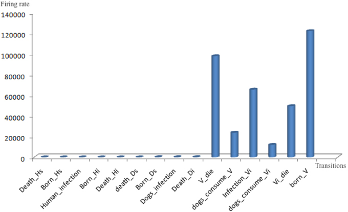
Figure 7. Cumulative firing rates of each transition in the T. Cruzi model during the whole simulation period of 30 years. Transitions representing processes operating on humans and dogs are very slow compared to the other transitions operating on vectors.

TABLE 3

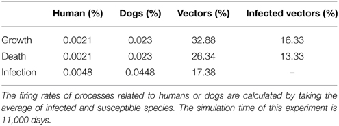
Table 3. Comparison of the cumulative transition firing rates (in percentage) of the model in Figure 4.

The simulation statistics in Table 3 show that growth and death of humans and dogs occur infrequently compared with the death and growth of vectors. For instance, the total firing rates of human growth and death is 0.0021%, compared to 32.88% for the growth rate of vectors. The reason for such a difference is that over a period of 30 years the age of humans and dogs is much larger than the age of bugs. Similarly, the accumulative firing rates of human and dog infections are very low in comparison with the firing rate of vector infections. This is a result of the abundance of the vector population in comparison with the human and dog populations.

Furthermore, the statistics in Figure 7 and Table 3 suggest that slow firing processes can be better represented by stochastic transitions, while faster ones should be better modeled via continuous transitions. Therefore, in Figure 4 all processes related to human and dog populations (e.g., growth, death, and infection) are modeled using stochastic transitions. In contrast, vector-related processes (e.g., vector growth, vector death, and vector infection) are modeled via continuous transitions.

To examine the implication of introducing stochastic transitions to the Chagas disease model, we compare the time course simulation result produced by the purely deterministic approach with the result of the hybrid simulator. Figures 8, 9 give the time course simulation results of the population of dogs and infected vectors simulated using both the deterministic and hybrid simulation techniques.

FIGURE 8

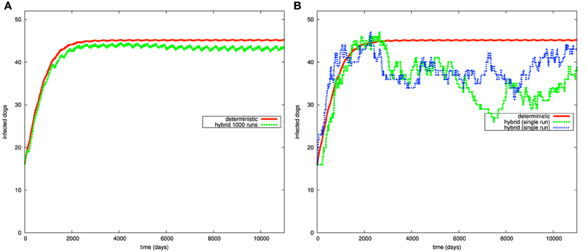
Figure 8. Simulation results of the Chagas model in Figure 4 for the dog population: (A) continuous and average hybrid time course result (1000 runs), (B) deterministic and two single runs of hybrid simulation.

FIGURE 9

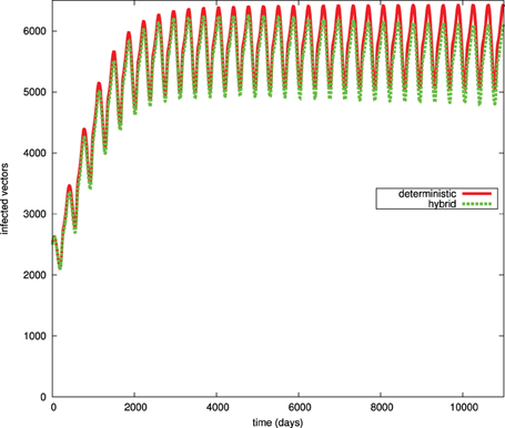
Figure 9. Simulation results for the infected vector population (V_i) in the deterministic and hybrid setting. V_i oscillates in the hybrid setting at slightly lower amplitude than in the purely deterministic setting.

In Figure 8A, the population of infected dogs implies the same qualitative conclusions for the deterministic and hybrid results. Both simulation results suggest that the population of infected vectors oscillates with respect to time. However, they differ in the specific quantitative values. Hybrid simulation results imply that the population of infected dogs enter the steady state at a lower value compared with the simulation results produced by the deterministic approach.

To better understand such differences in the quantitative results, we compare the results of the ODE approach with the individual runs of the hybrid simulation. Figure 8B presents two single runs of the hybrid simulation. These individual runs show that the population of infected dogs fluctuates as the result of simulating growth, death, and infection processes via stochastic transitions. In fact, modeling such processes in this way is more natural than using the deterministic approach to simulate them. Indeed, growth, death, and infection of dogs and humans are inherently stochastic processes. Moreover, the relatively small population of dogs motivates the use of stochastic transitions to simulate this type of processes.

To examine the influence of such fluctuation on the population of dogs and humans and on the rest of those model components, which remain modeled using the ODE approach, we plot the simulation results of infected vectors for the purely deterministic and the hybrid simulation results. Figure 9 shows that the population of infected vectors produced through the hybrid simulation technique oscillates at a lower amplitude than the purely deterministic counterpart. This implies that the noise related to the stochastically modeled part also influences the deterministically simulated components.

In summary, although deterministic and hybrid simulation techniques applied to the Chagas disease provide similar qualitative conclusions, the latter technique exhibits more accurate results due to the more realistic representation and simulation of inherently fluctuating natural processes.

Discussion

In this paper we propose the utilization of a special class of hybrid Petri nets, Generalized hybrid Petri nets, for the modeling and simulation of multi-timescale environmental systems. provide flexible and rich modeling features to represent and execute the different processes that are frequently encountered during the construction of dynamic models to explore environmental systems. The major advantage of using Petri nets compared with other techniques to represent and simulate environmental models is the graphical depiction of the system components' interactions supporting the communication in a multidisciplinary research team. Hybrid Petri nets extend the modeling power of standard Petri nets by providing a number of specific elements that can be used to represent physical processes operating at different timescales, which subsequently widens the classes of models that can make use of the Petri net approach and its unifying power.

The case study presented in the Result section explains the motivation behind the different elements of . For instance, read and inhibitor arcs are used to define boundary conditions for time periods, where vector mortality rates behave in a certain way (increasing or decreasing). Discrete transitions like immediate and deterministically delayed ones can be used to model the duration of time periods. The chosen case study, the Chagas model, involves processes that occur at different scales making the hybrid simulation technique most appropriate to execute such models. In this paper, the processes related to humans and dogs are represented by stochastic transitions. The effects of the other processes could also be investigated by modeling them as stochastic transitions. However, this would increase the simulation runtime for the model. In fact, provide a favorable tradeoff between a simulation's accuracy and runtime.

The discussed case study is implemented using the Petri net tool Snoopy (Heiner et al., 2012) which supports the construction and simulation of different Petri net classes including stochastic, continuous, and hybrid Petri nets. Snoopy can be download free of charge for academic use from Snoopy (2015). A model constructed with Snoopy can be simulated via a purely deterministic, stochastic, or hybrid simulator. This feature permits to experiment with different simulation techniques using one and the same model. We applied this specific feature to execute the case study in this paper using the deterministic and the hybrid simulator. Besides, a model constructed in Snoopy can be remotely simulated via Snoopy's Simulation and Steering Server (S⁴) (Herajy and Heiner, 2014a,b). S⁴ provides a further flexible tool to remotely simulate and steer Petri net models constructed using Snoopy. The Snoopy file implementing this model can be downloaded from http://www-dssz.informatik.tu-cottbus.de/DSSZ/Software/Examples. Thus, all our results presented in this paper are reproducible.

In the original model of Coffield et al. (2013), the vector growth rate at time t depends on the hatching rate at a previous time t − τ. The value of τ is approximated to be 20 days (Spagnuolo et al., 2011). This can be simulated as a delayed differential equation with a constant delay. In the discrete world, this delay can be accounted for in the model semantics using a deterministically time delayed transition with a delay of 20 days. However, using continuous transitions to simulate the growth rate of vectors, we need to adjust the semantics of such a transition type to take into account such a delay period while generating and solving the corresponding system of ODEs. This could be added in a future extension of the continuous Petri nets in Snoopy.

Author Contributions

The authors of this paper have equally contributed to the manuscript preparation.

Conflict of Interest Statement

The authors declare that the research was conducted in the absence of any commercial or financial relationships that could be construed as a potential conflict of interest.

Acknowledgments

This work has been partially funded by the GE-SEED grant (7934) which is administrated by STDF (Science and Technology Development Fund) and DAAD (German Academic Exchange Service).

Supplementary Material

The Supplementary Material for this article can be found online at: https://www.frontiersin.org/article/10.3389/fenvs.2015.00053

Supplemental Data

Supplemental material (S1) contains the constant coefficients required to specify transition rates of the Chagas disease model.

References

Ajmone, M., Balbo, G., Conte, G., Donatelli, S., and Franceschinis, G. (1995). Modelling with Generalized Stochastic Petri Nets. Wiley Series in Parallel Computing, John Wiley and Sons.

Google Scholar

Alla, H., and David, R. (1998). Continuous and hybrid Petri nets. J. Circ. Syst. Comp. 8, 159–188. doi: 10.1142/S0218126698000079

CrossRef Full Text | Google Scholar

Castañera, M. B., Aparicio, J. P., and Gürtler, R. E. (2003). A stage-structured stochastic model of the population dynamics of triatoma infestans, the main vector of Chagas disease. Ecol. Model. 162, 33–53. doi: 10.1016/S0304-3800(02)00388-5

CrossRef Full Text | Google Scholar

Coffield, D. J. Jr., Spagnuolo, A. M., Shillor, M., Mema, E., Pell, B., Pruzinsky, A., et al. (2013). A model for Chagas disease with oral and congenital transmission. PLoS ONE 8:e67267. doi: 10.1371/journal.pone.0067267

PubMed Abstract | CrossRef Full Text | Google Scholar

Cohen, J. E., and Gürtler, R. E. (2001). Modeling household transmission of american trypanosomiasis. Science 293, 694–698. doi: 10.1126/science.1060638

PubMed Abstract | CrossRef Full Text | Google Scholar

David, R., and Alla, H. (2010). Discrete, Continuous, and Hybrid Petri Nets. Berlin; Heidelberg: Springer.

Google Scholar

Fujita, S., Matsui, M., Matsuno, H., and Miyano, S. (2004). Modeling and simulation of fission yeast cell cycle on hybrid functional Petri net. IEICE Trans. Fundam. Electron. Commun. Comput. Sci. E87-A, 2919–2927.

Google Scholar

Gilbert, D., and Heiner, M. (2006). “From Petri nets to differential equations - an integrative approach for biochemical network analysis,” in Proc. ICATPN 2006, Vol. 4024, of LNCS, eds S. Donatelli and P. S. Thiagarajan (Berlin; Heidelberg: Springer), 181–200.

Google Scholar

Gillet, F. (2008). Modelling vegetation dynamics in heterogeneous pasture-woodland landscapes. Ecol. Model. 217, 1–18. doi: 10.1016/j.ecolmodel.2008.05.013

CrossRef Full Text | Google Scholar

Gregorio, S. D., Serra, R., and Villani, M. (1999). Applying cellular automata to complex environmental problems: the simulation of the bioremediation of contaminated soils. Theor. Comput. Sci. 217, 131–156. doi: 10.1016/S0304-3975(98)00154-6

CrossRef Full Text | Google Scholar

Heiner, M., Herajy, M., Liu, F., Rohr, C., and Schwarick, M. (2012). “Snoopy – a unifying Petri net tool,” in Proc. PETRI NETS 2012, Vol. 7347, of LNCS, eds S. Haddad and L. Pomello (Berlin; Heidelberg: Springer), 398–407.

Google Scholar

Herajy, M., and Heiner, M. (2012). Hybrid representation and simulation of stiff biochemical networks. J. Nonlin. Anal. 6, 942–959. doi: 10.1016/j.nahs.2012.05.004

CrossRef Full Text | Google Scholar

Herajy, M., and Heiner, M. (2014a). Petri net-based collaborative simulation and steering of biochemical reaction networks. Fundam. Informa. 129, 49–67. doi: 10.3233/FI-2014-960

CrossRef Full Text | Google Scholar

Herajy, M., and Heiner, M. (2014b). “A steering server for collaborative simulation of quantitative Petri nets,” in Application and Theory of Petri Nets and Concurrency, Vol. 8489, of Lecture Notes in Computer Science, eds G. Ciardo and E. Kindler (Switzerland: Springer International Publishing), 374–384.

Google Scholar

Herajy, M., Schwarick, M., and Heiner, M. (2013). Hybrid Petri Nets for modelling the eukaryotic cell cycle. ToPNoC VIII, 123–141. doi: 10.1007/978-3-642-40465-8/7

CrossRef Full Text | Google Scholar

Khoury, D. S., Barron, A. B., and Myerscough, M. R. (2013). Modelling food and population dynamics in honey bee colonies. PLoS ONE 8:e59084. doi: 10.1371/journal.pone.0059084

CrossRef Full Text | Google Scholar

Liu, H., Benoit, G., Liu, T., Liu, Y., and Guo, H. (2015). An integrated system dynamics model developed for managing lake water quality at the watershed scale. J. Environ. Manage. 155, 11–23. doi: 10.1016/j.jenvman.2015.02.046

PubMed Abstract | CrossRef Full Text | Google Scholar

Mao, G., and Petzold, L. (2002). Efficient integration over discontinuities for differential-algebraic systems. Comput. Math. Appl. 43, 65–79. doi: 10.1016/S0898-1221(01)00272-3

CrossRef Full Text | Google Scholar

Matsuno, H., Tanaka, Y., Aoshima, H., Doi, A., Matsui, M., and Miyano, S. (2003). Biopathways representation and simulation on hybrid functional Petri net. In Silico Biol. 3, 389–404.

PubMed Abstract | Google Scholar

Murata, T. (1989). Petri nets: properties, analysis and applications. Proc. IEEE 77, 541–580. doi: 10.1109/5.24143

CrossRef Full Text | Google Scholar

Nouvellet, P., Cucunubá, Z. M., and Gourbière, S. (2015). “Chapter four - ecology, evolution and control of Chagas disease: a century of neglected modelling and a promising future,” in Mathematical Models for Neglected Tropical Diseases: Essential Tools for Control and Elimination, Part A, Vol. 87, of Advances in Parasitology, eds R. M. Anderson and M. G. Basez (Academic Press), 135–191.

Qi, C., and Chang, N.-B. (2011). System dynamics modeling for municipal water demand estimation in an urban region under uncertain economic impacts. J. Environ. Manage. 92, 1628–1641. doi: 10.1016/j.jenvman.2011.01.020

PubMed Abstract | CrossRef Full Text | Google Scholar

Reddy, V., Mavrovouniotis, M., and Liebman, M. (1993). “Petri net representations in metabolic pathways,” in Proceedings of the 1st International Conference on Intelligent Systems for Molecular Biology, eds L. Hunter, D. Searls, and J. Shavlik (Bethesda, MD: The AAAI Press), 328–336.

Russell, S., Barron, A. B., and Harris, D. (2013). Dynamic modelling of honey bee (Apis mellifera) colony growth and failure. Ecol. Model. 265, 158–169. doi: 10.1016/j.ecolmodel.2013.06.005

CrossRef Full Text | Google Scholar

Schmickl, T., and Crailsheim, K. (2007). Hopomo: a model of honeybee intracolonial population dynamics and resource management. Ecol. Model. 204, 219–245. doi: 10.1016/j.ecolmodel.2007.01.001

CrossRef Full Text | Google Scholar

Seppelt, R., Müller, F., Schröder, B., and Volk, M. (2009). Challenges of simulating complex environmental systems at the landscape scale: a controversial dialogue between two cups of espresso. Ecol. Model. 220, 3481–3489. doi: 10.1016/j.ecolmodel.2009.09.009

CrossRef Full Text | Google Scholar

Snoopy (2015). Snoopy Website. Available online at: http://www-dssz.informatik.tu-cottbus.de/snoopy.html[Accessed: 28/3/2015].

Soliman, S., and Heiner, M. (2010). A unique transformation from ordinary differential equations to reaction networks. PLoS ONE 5:e14284. doi: 10.1371/journal.pone.0014284

PubMed Abstract | CrossRef Full Text | Google Scholar

Spagnuolo, A., Shillor, M., and Stryker, G. (2011). A model for Chagas disease with controlled spraying. J. Biol. Dyn. 5, 299–317. doi: 10.1080/17513758.2010.505985

PubMed Abstract | CrossRef Full Text | Google Scholar

Tian, Z., Faure, A., Mori, H., and Matsuno, H. (2013). Identification of key regulators in glycogen utilization in E. coli based on the simulations from a hybrid functional Petri net model. BMC Syst. Biol. 7:S1. doi: 10.1186/1752-0509-7-S6-S1

PubMed Abstract | CrossRef Full Text | Google Scholar

Uusitalo, L., Lehikoinen, A., Helle, I., and Myrberg, K. (2015). An overview of methods to evaluate uncertainty of deterministic models in decision support. Environ. Model. Soft. 63, 24–31. doi: 10.1016/j.envsoft.2014.09.017

CrossRef Full Text | Google Scholar

Valk, R. (1978). “Self-modifying nets, a natural extension of Petri nets,” in Proc. of the Fifth Colloquium on Automata, Languages and Programming (London, UK: Springer-Verlag), 464–476.

Google Scholar

Xiang, J., Chen, H., and Ishikawa, H. (2013). A mathematical model for the transmission of schistosoma japonicum in consideration of seasonal water level fluctuations of Poyang Lake in Jiangxi, China. Parasitol. Int. 62, 118–126. doi: 10.1016/j.parint.2012.10.004

PubMed Abstract | CrossRef Full Text | Google Scholar