Renormalization Group for Critical Phenomena in Complex Networks

We discuss the behavior of statistical models on a novel class of complex “Hanoi” networks. Such modeling is often the cornerstone for the understanding of many dynamical processes in complex networks. Hanoi networks are special because they integrate small-world hierarchies common to many social and economical structures with the inevitable geometry of the real world these structures exist in. In addition, their design allows exact results to be obtained with the venerable renormalization group (RG). Our treatment will provide a detailed, pedagogical introduction to RG. In particular, we will study the Ising model with RG, for which the fixed points are determined and the RG flow is analyzed. We show that the small-world bonds result in non-universal behavior. It is shown that a diversity of different behaviors can be observed with seemingly small changes in the structure of hierarchical networks generally, and we provide a general theory to describe our findings.

1. Introduction

The renormalization group (RG; Wilson, 1971; Wilson and Fisher, 1972) is by now a method found in any “classical” statistical physics text book (Goldenfeld, 1992; Plischke and Bergersen, 1994). It has allowed to categorize broad classes of equilibrium systems into an enumerable set of universality classes, each characterized by discrete features, such as their dimension and the symmetries adhered to by their Hamiltonians (Goldenfeld, 1992; Plischke and Bergersen, 1994). Such universality is made possible through the property of “scaling” that is an inherent feature near phase transitions (Kadanoff, 1966), which these systems undergo in certain regions of the space spanned by their physical parameters (couplings). Scaling invariance entails that system-specific details on the microscopic level become irrelevant, as the behavior over many orders in the range of the interactions become self-similar. In this framework, analogous behavior in a surprisingly wide set of phenomena, such as the condensation of fluids, spontaneous magnetization of materials, or the generation of particle mass in the early universe, can be described in a single effective theory; certainly a major intellectual accomplishment of modern physics across all fields (Goldenfeld, 1992).

In the past 15 years, statistical physicist have increasingly applied the ideas of critical phenomena and scaling to problems outside of the immediate material realm, in newly emerging fields such as “Econophysics,” “Sociophysics,” etc. (Mantegna and Stanley, 1999; Barabasi, 2003; Kleinert, 2004). The considered systems typically feature a large number of interacting agents sharing a finite set of intrinsic properties on account of which they interact. But unlike in a Euclidean defined arrangement of “actors” in a physical system, such as atoms in a material, these systems possess a more complex network of mutual interactions (which may even be directed; Watts and Strogatz, 1998; Boccaletti et al., 2006; Dorogovtsev et al., 2008). Thus, in many respects, the study of these phenomena is inseparable from the understanding of the geometry of networks (Barthelemy, 2011). One major accomplishment of these investigations is the realization that many of the networks that are engineered by some natural or human activity themselves exhibit emergent complex properties, for instance, as found in the scale-free degree distribution of the internet.

But while these networks, or dynamical systems on them, may behave critically, many of these phenomena were soon found to be non-universal. For instance, in the preferential attachment model for the world-wide net (Barabasi and Albert, 1999), the value of the scaling exponent is tied to microscopic details of the attachment rule. In this sense, it would seem unlikely that any sweeping classification scheme could be devised to categorize this amorphous pile of particulars. Here, we will attempt a foray into such a scheme, albeit limited to those classical equilibrium phenomena, but on a large set of different networks. We suspect that our discussion might help to explain, for example, a number of similar observations of traditionally obscure critical behaviors, such as infinite-order transitions, in very different network models, in and out of equilibrium (Dorogovtsev et al., 2008).

Our classification scheme is best introduced with a variety of hierarchical networks on which RG is exact, and the critical phenomena can be studied in great detail. Metric version of such networks, such as that introduced in the Migdal-Kadanoff RG, provide the classical text-book examples of RG and universality (Berker and Ostlund, 1979; Goldenfeld, 1992; Plischke and Bergersen, 1994; Hinczewski and Berker, 2006). But in the advent of complex networks, many hierarchical designs with non-metric (i.e., small-world or scale-free) properties have been devised and studied (Andrade et al., 2005; Hinczewski and Berker, 2006; Hinczewski, 2007; Boettcher and Goncalves, 2008; Boettcher et al., 2008). Our study shows that criticality in many of these models (percolation, Ising, etc.) is definitely non-universal but falls into a few (here, three) generic regimes, each characterized by its degree of singularity in, say, the correlation length at the critical point (Boettcher and Brunson, 2011). One of these regimes is indeed an infinite-order transition reminiscent of that described by Berezinskii and Kosterlitz and Thouless (BKT; Goldenfeld, 1992; Plischke and Bergersen, 1994). It is flanked on one side by a transition with a “weaker,” algebraic divergence, similar to the classical ones of second order (but still non-universal), and on the other by a regime with a fully essential singularity. These regimes are defined through the relative strength of (non-Euclidean) long-range or small-world bonds in one and the same network, with clear demarcations between these regimes as a function of that coupling strength.

In the following Section 2, we describe the Hanoi networks. The analysis of the phase diagrams and the RG flow for the Ising ferromagnet on these networks is discussed in Sections 3 and 4. In Section 5, we introduce families of interpolating networks to reveal a more comprehensive set of regimes, each with its own characteristic type of phase transition, and we conclude with a discussion of our results in their implications in Section 7.

2. Geometry of the Hanoi Networks

Each of the Hanoi network possesses a simple geometric backbone, a one-dimensional line of sites n, 0 ≤ n ≤ N = 2^k (k → ∞). Each site is connected to its nearest neighbor, ensuring the existence of the 1d-backbone. To generate the small-world hierarchy in these networks, consider parameterizing any integer n (except for zero) uniquely in terms of two other integers (i, j), i ≥ 0, via

Here, i denotes the level in the hierarchy whereas j ≥ 0 labels consecutive sites within each hierarchy. For instance, i = 0 refers to all odd integers, i = 1 to all integers once divisible by 2 (i.e., 2, 6, 10,…), and so on. Depending on its level of the hierarchy, any site has also small-world (i.e., long-range) bonds to more-distant sites along the backbone, according to some deterministic rule. For example, we obtain a 3-regular network HN3 by connecting also 1 to 3, 5 to 7, 9 to 11, etc., for i = 0, next 2 to 6, 10 to 14, etc., for i = 1, and 4 to 12, 20 to 28, etc., for i = 2, and so on, as depicted in Figure 1.

FIGURE 1

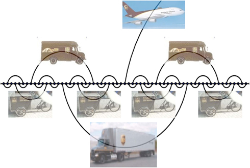
Figure 1. Depiction of the 3-regular network HN3 on a semi-infinite line, here drawn suggestively as a model for hierarchically organized transport. Many goods and services are distributed in a small-world hierarchical manner before they get delivered in a real-world geometry.

While HN3 (and HN4 Boettcher et al., 2008) are of a fixed, finite degree, we introduced here convenient generalizations of HN3 that lead to new, revealing insights into small-world phenomena. First, we can extend HN3 in the following manner to obtain a new planar network of average degree 5, hence called HN5: In addition to the bonds in HN3, in HN5 we also connect all even sites to both nearest sites within the same level of the hierarchy i(≥1). The resulting network remains planar but now sites have a hierarchy-dependent degree, as shown in Figure 2. It is easy to show that the average shortest path between any two sites increases in HN3, and logarithmically in HN5, with system size N.

FIGURE 2

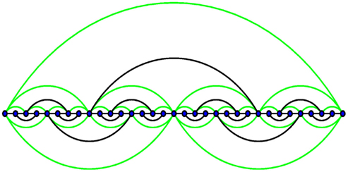
Figure 2. Depiction of the planar network HN5, comprised of HN3 (black lines) with the addition of further long-range bonds (green-shaded lines). Note that sites on the lowest level of the hierarchy have degree 3, then degree 5, 7, etc., comprising a fraction of 1/2, 1/4, 1/8, etc., of all sites, which makes for an average degree 5 in this network.

3. Ising Ferromagnet on HN3

The RG consists of recursively tracing out spins level-by-level in the hierarchy (Boettcher et al., 2008). In terms of Eq. (1), we start by tracing out all sites with n odd, i.e., i = 0, then those n which are divisible by 2 only once, i.e., i = 1, and so on. We can always relabel all sites n after any RG step by n → n/2, so that we trace out the respective odd-relabeled sites at any level. It is apparent, for instance from Figure 1, that odd-labeled sites are connected to their even-labeled nearest neighbors on the backbone, say, by a coupling K₀(=βJ₀). At any level, each odd-labeled site x_{n ± 1} is also connected to one other such site across an even-labeled site x_n with n = 2(2j + 1) that is exactly once divisible by 2. Let us call that coupling K₁(=βJ₁). The basic RG step is depicted in Figure 3 and consists of tracing out the two sites x_{n ± 1} neighboring the site x_n for all j with n = 2(2j + 1).

FIGURE 3

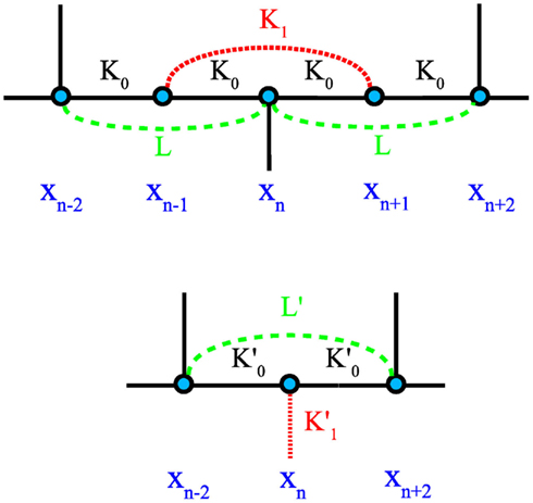
Figure 3. Depiction of the (exact) RG step for the Ising model on HN3. The step consists of tracing out odd-labeled variables x_{n ± 1} in the top plot and expressing the renormalized couplings on the bottom in terms of the old couplings (L, K₀, K₁). Note that the original network in Figure 1 does not contain couplings of type (L, L′), but that they certainly become relevant during the process.

We can section the Ising Hamiltonian

where ℛ contains all coupling terms of higher level in the hierarchy, and each sectional Hamiltonian is given by

where (K₀, K₁, L) are the unrenormalized couplings defined in Figure 3 and I is a constant that fixes the overall energy scale per spin. (There are effectively 4 spins involved in each graph-let, as those at each boundary are equally shared with neighboring graph-lets.) While couplings of the type L₀ between next-nearest even-labeled neighbors emerges that are not part of the network initially in HN3, they do emerge during the RG step (otherwise the system of recursion equations would not close), see Figure 3.

To simplify the analysis, we introduce new variables similar to inverse “activities” (Plischke and Bergersen, 1994),

which ensure that the RG flow only contains algebraic functions and, for the ferromagnetic model, remains confined within the physical domain 0 ≤ κ, λ, μ ≤ 1. Thus, we rewrite Eq. (3) as

Tracing out the odd-labeled spins, we have to evaluate

for the remaining spins in terms of the renormalized quantities C′, κ′, λ′. Of the eight possible relations resulting from the combinations x_{n − 2}, x_n, x_{n + 2} = ± 1, only three are independent. After some algebra, we extract from those the RG recursions:

Note that for couplings in higher levels of the hierarchy it is for i ≥ 1; correspondingly, these couplings, and hence, μ, will not renormalize. Instead, they retain their “bare” value μ² determined by the temperature, kT/J = − 2/ ln μ. In this sense, we will use μ as a measure of temperature throughout.

Only half of the contribution to the renormalized energy scale is originating with the sectional Hamiltonian in Eq. (5), since at the next level two such sections are combined into one, making C′ ∝ C². While we do not consider the recursions for C in this paper, they are essential to reconstruct the free energy for each system, and will be analyzed elsewhere (Boettcher and Brunson, unpublished).

Equation (7) provide recursions order-by-order in the RG for the evolution of the effective couplings characterizing increasingly larger scales of the network. To facilitate this RG flow, we need to specify initial conditions for a particular physical situation realized in the unrenormalized, bare network. Here, we restrict ourselves to networks with uniform bonds (although many interesting choices are conceivable, such as distance-dependence; Kotliar et al., 1983; Katzgraber, 2003; Hinczewski and Berker, 2006). For HN3 this implies that we chose J = 1 as our energy scale, such that K_i = βJ = β and I = L₀ = 0 initially, or in terms of Eq. (4);

Searching for fixed points and L′ = L = L*, i.e., κ′ = κ = κ* and λ′ = λ = λ* in Eq. (7), immediately provides the trivial, high-temperature solution κ* = λ* = 1, i.e., Further analysis yields only a line of (unstable) strong-coupling fixed points,

extending from for low temperatures, μ = 0, to λ* = 1 for T → ∞, where μ = 1. Even at T = 0, only the renormalized backbone bonds K₀ provide strong coupling, the emerging long-range bonds L₀ only exert limited coupling strength.

Local analysis near the fixed points with the Ansatz

reveals that the high-temperature fixed point is always stable and corrections decay exponentially, where the exponential contains a factor of At the low-temperature line of fixed points in Eq. (9) we find

which is divergent for all T > 0, i.e., 0 < μ ≤ 1, making the fixed point at T = 0 unstable. For any fixed point, there is no linear expansion possible that would yield critical exponents. For the initial conditions in Eq. (8), corresponding to uniform couplings throughout the unrenormalized network, the RG flow always evolves to the high-temperature fixed point. Thus, the ferromagnet on this network behaves similar to a 1d Ising model.

4. Ising Ferromagnet on HN5

As shown in Section 2, HN5 is basically an extension of HN3, created by adding a new layer of links to each level of the hierarchy. As is apparent from the foregoing discussion in 3, these additions correspond precisely to new renormalizable operators (here, the bonds L) that inevitably emerge during the RG of HN3, see Figure 3. In HN5, these new operators are simply deemed an original feature of the network, hence, maintaining the RG as an exact procedure. Consequently, the RG itself hardly changes, see Figure 4; it merely differs by one extra link in the graph-let, L₁, compared to that for HN3 in Figure 3. In Eq. (3), it only adds the term L_{1xn − 2xn + 2} to the sectional Hamiltonian and, like L₀ itself, L₁ does not get traced over in the calculation in Eq. (6). We can introduce these new bonds as yet another free, non-renormalizing coupling in the RG and choose, to wit,

FIGURE 4

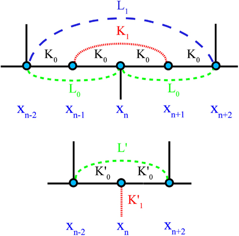
Figure 4. Depiction of the (exact) RG step for the Ising model on HN5. This step is identical to that for HN3 in Figure 3 aside from the extra link L₁ spanning between x_{n − 2} and x_{n + 2} (top), which contributes to the renormalization of (bottom).

This merely contributes a factor of to the unprimed side of Eq. (6), which correspondingly alters only the recursion for λ′ in Eq. (7) by a factor of μ^2y. Otherwise using the same definitions as in Section 3, we obtain the RG recursions for the Ising ferromagnet on HN5:

Accordingly, due to the bare existence of the L₁ bond, we will have to change the initial conditions from Eq. (8) to

Analyzing these recursions for fixed points, κ′ = κ = κ* and λ′ = λ = λ*, we find that the addition of the extra long-range bond has eliminated the high-temperature fixed point found in HN3. At low temperatures, we find similar to Eq. (9) in HN3 a line of fixed points

which here extends over the entire domain for the long-range bonds, 0 ≤ λ* ≤ 1 for 0 ≤ μ ≤ 1. Note that although y represents a continuous interpolation between HN3 and HN5, there is a singular limit at y → 0 toward an isolated point corresponding to HN3, see Eq. (9). In the following, we only treat the case of couplings that are homogeneous throughout the unrenormalized network, y = 1. Consideration of the rich set of transitions occurring for the family of networks parameterized by interpolating 0 < y ≤ 1 is deferred to Section 5.

Dividing out the κ* = 0-solution, further analysis of Eq. (13) for y = 1 reveals yet another line of fixed points given by

which can be expressed most simply in closed form as

by eliminating μ. As we will see, these relations lead to physical fixed points only within a limited range of the temperature μ. The phase diagram for the backbone coupling κ in HN5 at y = 1 can be found in Figure 5. Blue arrows indicate the RG flow for the initial conditions in Eq. (14), which starts on the diagonal, representing all-equal bonds for the homogeneous network. For these initial conditions, the flow always evolves toward smaller values of κ, i.e., stronger coupling. But there is a notable transition where the attained fixed-point jumps from the low-temperature branch in Eq. (15) characterized by κ* = 0, i.e., a solidly frozen backbone, to the branch given Eq. (17) on which κ* (as well as λ*) becomes finite. We obtain this transition point by evaluating Eqs. (16, 17) for κ* = 0, which yields λ* = 1/2ɸ = 0.309017…, giving a critical temperature of

FIGURE 5

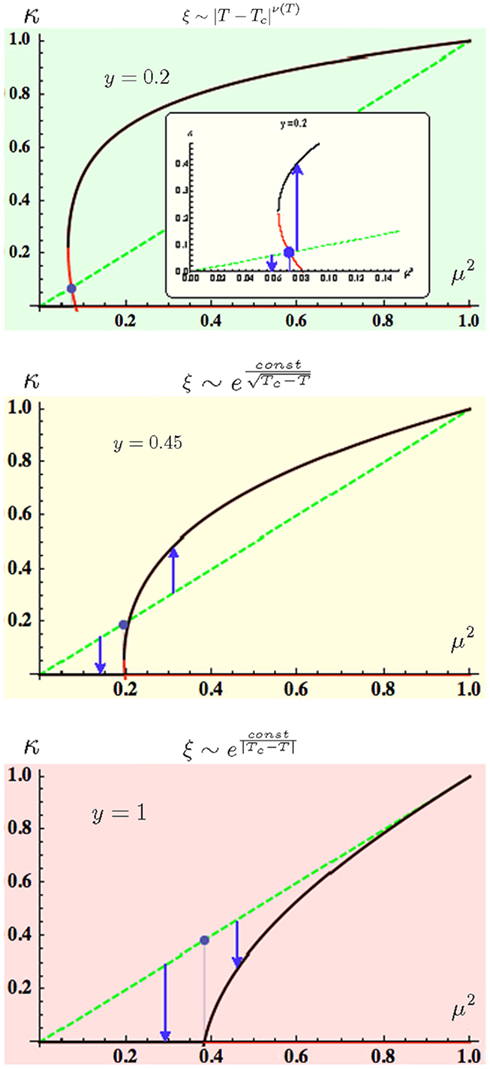
Figure 5. Plot of κ* in Eq. (19) as a function of μ² for y as defined in Eq. (12). The generic cases are represented by y = 0.2 (top), y = 0.45 (middle), and the case of HN5 discussed in Section 4 for y = 1 (bottom), for which the branch-point (BP) has “sunset” out of the physical regime. In all cases, the dashed, green-shaded line indicates the initial conditions (IC) for the RG flow in Eqs. (13, 14), κ⁽⁰⁾ = μ². For μ fixed, the RG flow must proceed vertically, either up or down, to the nearest stable line of fixed points. For low y (top), the IC crosses the unstable branch below BP (see enlargement in the inset) which then can not be reached by the flow. Once the IC cross above BP (middle), the flow must pass BP, unless BP sunsets (bottom). For each case, the generic divergence is indicated for the correlation length ξ at T → T_c, as derived in Section 6.

where is the “golden ratio” (Boettcher and Goncalves, 2008). For bare couplings at this temperature, marked by a blue dot in the (y = 1)-plot of Figure 5, the RG flow marginally reaches the strong-coupling limit. In this network, for these initial conditions the RG flow never reaches an unstable fixed point such as the unstable portion of Eq. (15), marked by a red-shaded line in Figure 5. As we will see below, this situation will change when we weaken the impact of long-range couplings.

5. Interpolation between Hanoi Networks

We have already observed in the construction of HN5 in Section 4 that it is easy to promote the L-couplings that inevitably emerge during the RG to be associated with an actual bond in the network. Here, we will fully exploit this fact to obtain a one-parameter family of problems with various regimes of phase behaviors. In particular, we discover transitions between such regimes as a function of the parameter that will allow us to clarify the connections between the diverse set of behaviors that we have discovered in the previous section.

In Section 4, we argued for the introduction of small-world bonds with couplings L_i and developed the RG recursions in (13) assuming a relative strength of these couplings to those germane to HN3 of the form in Eq. (12). Here, we will now consider the behavior that results from varying the strength parameter y between the two extremes already explored, y = 0 for HN3 in Section 3 and y = 1 for HN5 in Section 4.

Analyzing these recursions in Eq. (13) for fixed points, we already found the low-temperature fixed-point line in Eq. (15). Dividing out this κ* = 0-solution, further analysis of Eq. (13) reveals a line of fixed points,

abbreviating the discriminant

For y → 0, this solution degenerates into the high-temperature fixed point of HN3. But for any finite y, these lines of fixed points are non-trivial functions of μ, as depicted for κ*(μ²) in Figure 5. The dominant feature in these plots is the root-singularity in κ* with a branch-point-separating the upper stable and lower unstable line of fixed points. Essentially, three distinct generic regimes can be discerned: (1) If the branch-point happens to lie below of the physical regime, we observe a phase transition without access to any unstable point (see bottom of Figure 5); a critical point akin to that for HN5 at y = 1 analyzed in Section 4 arises. If the branch-point rises into the physical regime, here for y < y_c = [ln(3/2)/ln2] = 0.584963…, then depending on whether the initial conditions of the RG flow cross the critical line below or above the branch-point, we find (2) a transition seemingly of finite-order on intercepting the unstable lower branch (see top of Figure 5) for which the RG flow never accesses the branch-point singularity. If, in turn, the initial conditions cross above, (3) a BKT-like transition results because the RG flow now must pass the singularity (see middle of Figure 5), as we will show below.

6. General Classification of Critical Regimes

Instead of the rather tedious analysis of the critical regimes resulting from Eq. (19) for a coupled set of variables (which can be found in Boettcher and Brunson, 2011), we rather take a step back and assess the larger picture here. It turns out to be easy to devise a simple theory¹ that reproduces all the previously found features in a generic way, thereby demonstrating the generality of this classification, not only accounting for other hierarchical networks (Andrade et al., 2005; Hinczewski and Berker, 2006; Hinczewski, 2007; Boettcher and Goncalves, 2008; Boettcher et al., 2008) but also for any physical system described by parameter-dependent renormalization group equations. Even systems on complex networks that have not been subjected to an RG treatment have been found to exhibit the peculiar infinite-order transitions found here (Dorogovtsev et al., 2008), and may eventually be related to this classification.

It is sufficient to consider the RG recursion for a single coupling, say, κ_n with some control parameter μ², defined as in Eq. (4), for instance. A conventional RG treatment (Goldenfeld, 1992; Plischke and Bergersen, 1994) for a system on a regular lattice leads to recursions that only depend on the evolving coupling itself. There, any parameter dependence, such as on the temperature for spin models or on the bond density for percolation problems, is limited to the initial conditions of the RG, which define the particular model being studied; they do not affect the properties near the fixed points. In contrast, inserting such a dependence influences the location of fixed points as well as the behavior near them. As the example displayed in Figure 5 suggests, even the very fixed point that controls the dynamics may depend on the initial conditions, violating any conventional sense of universality. Yet, if we assume that the most elementary, generic fixed-point topology that deviates from the conventional picture is represented by a root branch-point², we can classify all observed critical phenomena into just a few regimes. To wit, we write

This model of a generic RG recursion is cubic to ensure that, after extracting the trivial strong-coupling fixed point ³, the remaining fixed-point equations produce a root branch-point,

revealing the undetermined constant κ_b as the coupling strength found at the branch-point, which we may choose freely to place the branch-point inside (0 ≤ κ_b ≤ 1) or outside the physical regime. (Regarding Section 5, we could view κ_b = κ_b(y) as the quantity that specifies the family of models considered.) The function f (μ) captures the minimal parameter dependence of the model, as expressed through the μ-dependence of both branches of the fixed points . Here, f (μ) is a monotone rising function on the physical interval 0 ≤ μ ≤ 1, which may contain a zero, f (μ_b) = 0. Generically, it would have a simple Taylor expansion near μ_b, i.e., f (μ_b ± Δμ) ∼ ±Δμf ^′(μ_c) for small Δμ.

In light of Figure 5, the first two panels correspond to the case where both, κ_b and μ_b, are in the physical regime with a visible branch-point (although the RG recursions there are far more complicated); the last panel represents κ_b ≤ 0. The decisive difference between those first two panels is whether the location of the branch-point is above or below the line of initial conditions. Depending on the model, the line of initial conditions could be any monotone function of μ, possibly resulting in different critical behaviors in the way they pass by identical branch-points, but it is more convenient to imagine this line as a simple diagonal in the (μ², κ)-plane and move the branch-point instead. Within the physical regime, the lower fixed-point branch is always unstable while the upper remains stable, as a local analysis along each branch readily reveals. Stable and unstable fixed-point lines merge at the branch-point, where particularly interesting phenomena can arise.

In the case that long-range, hierarchical effects are weakest, as for the first panel in Figure 5, the branch-point is far on the right, and may even be outside to the right and/or above of the physical regime. Then, the initial conditions merely intersect the unstable branch at some point μ_c. The RG flow (vertical blue arrows in Figure 5) for 0 ≤ μ < μ_c advances toward strong coupling at , while for μ_c < μ ≤ 1 it flows toward , making μ_c the critical point. Note that only for μ → 1, reflecting the physical phenomenon of “patchiness” (Boettcher et al., 2009): hierarchical, long-range couplings enforce some semblance of order between otherwise uncorrelated (sub-extensive) patches of locally connected degrees of freedom even in the disordered regime; full disorder is often only reached at infinite temperature, dilution, etc. Near μ_c, all the critical dynamics of the system is then solely determined by the local properties of the unstable critical point that has be (non-universally) selected by the particular system via the initial conditions. As in a conventional system, local analysis (Goldenfeld, 1992; Plischke and Bergersen, 1994) similar to Eq. (10) but near with an Ansatz for ϵ_n ≪ 1 on Eq. (21) provides, e.g., the scaling exponent for the divergence of the correlation length,

except that the exponent is non-universal, evaluated at the crossing point μ_c (Boettcher and Brunson, 2011). The RG flow in this case never passes sufficiently near the branch-point singularity to be affected.

The other extreme, when long-range couplings dominate, leads to a picture similar to the last panel of Figure 5 but with κ_b < 0. No unstable fixed points can be reached for any choice of (physical) initial conditions. The RG flow always advances to the next best stable fixed point, either at strong coupling for 0 ≤ μ < μ_c, or toward patchy order at for μ_c < μ ≤ 1, making μ_c again the critical point. At μ_c, where both lines of stable fixed-points intersect, we find an exponentially divergent correlation length to signal the phase transition. The Ansatz for ϵ_n ≪ 1 on Eq. (21) provides

Since from expanding Eq. (22) near , we get

Thus, the correlation length diverges as

Again, the RG flow does not pass the branch-point singularity, as it is located outside (below) the physical domain.

Only in the intermediate regime, as represented by the middle panel of Figure 5, does the RG flow for some critical μ_c pass by the branch-point singularity, which then controls the critical behavior in a novel way. As before, for 0 ≤ μ < μ_c the flow reaches strong coupling at and patchy order at for μ_c < μ ≤ 1. A local analysis of the flow just below the critical point, μ ∼ μ_c − Δμ, with κ_n ∼ κ_b(1 + ϵ_n) for ϵ_n ≪ 1 on Eq. (21) yields

This relation exhibits a boundary layer, i.e., in the limit Δμ → 0 the solution drastically changes behavior. With the methods of Bender and Orszag (1978), we can transform into the “inner” boundary region by rescaling ϵ_n → ηϵ_n and n → δn applied to Eq. (27),

which becomes balanced for Accordingly, the characteristic width of the boundary layer scales with

which by Eq. (26) leads to the divergence in the correlation length characteristic of BKT,

Clearly, the physical origin of this singularity is not even remotely related to an actual BKT transition. In fact, instead of its rarity, confined to very particular lattice models, we may find it to be one of a few generic types of transition in networks.

7. Conclusion

We have analyzed the fixed-point structure of an Ising ferromagnet on a set of Hanoi networks with an exact real-space renormalization group. Using interpolating families of such networks, with the relative coupling strength between backbone and small-world bonds as the interpolation parameter, we reveal a number of regimes with distinct critical behaviors. While in each such regime the critical transition has non-universal features, the characteristics of the transition in each one has generic, robust features. For increasing strength, we observe that the divergence in the correlation length changes from a non-universal power-law |x|^−v, to a BKT-like essential singularity then to a full singularity e^1/x, on approach to the critical point x ∼ |μ_c − μ| → 0. We trace the changes from one regime to the next in terms of the analytic structure of the RG flow. Finding an enumerable range of such characteristics suggest a possible classification of critical behavior of statistical models in networks generally, for which we propose a general description. Similar critical properties of the kind found here have also been observed in percolation (Berker et al., 2009; Boettcher et al., 2009; Nogawa and Hasegawa, 2009; Hasegawa et al., 2010), for example. The existence of entire regimes that exhibit essential singularities in the divergence of the correlations, as we have found here, might explain the surprising prevalence of typically quite rare BKT-like transitions in otherwise unrelated network models (Dorogovtsev et al., 2008). In the analysis of, say, social interaction networks, which have been found to have a hierarchical structure (Trusina et al., 2004), it is therefore essential to be aware of the novel phenomena describe here.

Conflict of Interest Statement

The authors declare that the research was conducted in the absence of any commercial or financial relationships that could be construed as a potential conflict of interest.

Footnotes

1. ^Our approach is similar in spirit to Landau’s description of a mean-field phase transition found in any text book on critical phenomena (Goldenfeld, 1992; Plischke and Bergersen, 1994).
2. ^Of course, the simplest deviation from constant fixed points that are entirely independent of the parameter would be a linear dependence. However, such dependence can be subsumed into our model (by moving the branch cut far outside the physical domain, for instance).
3. ^For the weak-coupling fixed point it is sufficient to require that f(μ) is chosen such that in (Eq. 22).

References

Andrade, J. S., Herrmann, H. J., Andrade, R. F. S., and da Silva, L. R. (2005). Apollonian networks: simultaneously scale-free, small world, Euclidean, space filling, and with matching graphs. Phys. Rev. Lett. 94, 018702.

Pubmed Abstract | Pubmed Full Text | CrossRef Full Text

Barabasi, A.-L. (2003). Linked: How Everything is Connected to Everything Else and What it Means for Business, Science, and Everyday Life. New York: Plume.

Barabasi, A.-L., and Albert, R. (1999). Emergence of scaling in random networks. Science 286, 509.

Pubmed Abstract | Pubmed Full Text | CrossRef Full Text

Barthelemy, M. (2011). Spatial networks. Phys. Rep. 499, 1.

CrossRef Full Text

Bender, C. M., and Orszag, S. A. (1978). Advanced Mathematical Methods for Scientists and Engineers. New York: McGraw-Hill.

Berker, A. N., Hinczewski, M., and Netz, R. R. (2009). Critical percolation phase and thermal Berezinskii-Kosterlitz-Thouless transition in a scale-free network with short-range and long-range random bonds. Phys. Rev. E Stat. Nonlin. Soft Matter Phys. 80, 041118.

Pubmed Abstract | Pubmed Full Text | CrossRef Full Text

Berker, A. N., and Ostlund, S. (1979). Renormalisation-group calculations of finite systems: order parameter and specific heat for epitaxial ordering. J. Phys. Condens. Matter 12, 4961.

Boccaletti, S., Latora, V., Moreno, Y., Chavez, M., and Hwang, D.-U. (2006). Complex networks: structure and dynamics. Phys. Rep. 424, 175.

CrossRef Full Text

Boettcher, S., and Brunson, C. T. (2011). Fixed-point properties of the Ising ferromagnet on the Hanoi networks. Phys. Rev. E Stat. Nonlin. Soft Matter Phys. 83, 021103.

Pubmed Abstract | Pubmed Full Text | CrossRef Full Text

Boettcher, S., Cook, J. L., and Ziff, R. M. (2009). Patch percolation on a hierarchical network with small-world bonds. Phys. Rev. E Stat. Nonlin. Soft Matter Phys. 80, 041115.

Pubmed Abstract | Pubmed Full Text | CrossRef Full Text

Boettcher, S., and Goncalves, B. (2008). Anomalous diffusion on the Hanoi networks. Europhys. Lett. 84, 30002.

CrossRef Full Text

Boettcher, S., Gonçalves, B., and Guclu, H. (2008). Hierarchical regular small-world networks. J. Phys. A Math. Theor. 41, 252001.

CrossRef Full Text

Dorogovtsev, S. N., Goltsev, A. V., and Mendes, J. F. F. (2008). Critical phenomena in complex networks. Rev. Mod. Phys. 80, 1275.

CrossRef Full Text

Goldenfeld, N. (1992). Lectures on Phase Transitions and the Renormalization Group. Reading: Addison-Wesley.

Hasegawa, T., Sato, M., and Nemoto, K. (2010). Generating-function approach for bond percolation in hierarchical networks. Phys. Rev. E Stat. Nonlin. Soft Matter Phys. 82, 046101.

Pubmed Abstract | Pubmed Full Text | CrossRef Full Text

Hinczewski, M. (2007). Griffiths singularities and algebraic order in the exact solution of an Ising model on a fractal modular network. Phys. Rev. E Stat. Nonlin. Soft Matter Phys. 75, 061104.

Pubmed Abstract | Pubmed Full Text | CrossRef Full Text

Hinczewski, M., and Berker, A. N. (2006). Inverted Berezinskii-Kosterlitz-Thouless singularity and high-temperature algebraic order in an Ising model on a scale-free hierarchical-lattice small-world network. Phys. Rev. E Stat. Nonlin. Soft Matter Phys. 73, 066126.

Pubmed Abstract | Pubmed Full Text | CrossRef Full Text

Kadanoff, L. P. (1966). Scaling laws for Ising models near Tc. Physics 2, 263.

Katzgraber, H. G., and Young, A. P. (2003). Monte Carlo studies of the one-dimensional Ising spin glass with power-law interactions. Phys. Rev. B Condens. Matter Mater. Phys. 67, 134410.

CrossRef Full Text

Kleinert, H. (2004). Path Integrals in Quantum Mechanics, Statistics, Polymer Physics, and Financial Markets. Singapore: World Scientific.

Kotliar, G., Anderson, P. W., and Stein, D. L. (1983). One-dimensional spin-glass model with long-range random interactions. Phys. Rev. B Condens. Matter Mater. Phys. 27, R602.

CrossRef Full Text

Mantegna, R. N., and Stanley, H. E. (1999). An Introduction to Econophysics: Correlations and Complexity in Finance. Cambridge: Cambridge University Press.

Nogawa, T., and Hasegawa, T. (2009). Monte Carlo simulation study of the two-stage percolation transition in enhanced binary trees. J. Phys. A Math. Theor. 42, 145001.

CrossRef Full Text

Plischke, M., and Bergersen, B. (1994). Equilibrium Statistical Physics, 2nd Edn. Singapore: World Scientific.

Trusina, A., Maslov, S., Minnhagen, P., and Sneppen, K. (2004). Hierarchy measures in complex networks. Phys. Rev. Lett. 92, 178702.

Pubmed Abstract | Pubmed Full Text | CrossRef Full Text

Watts, D. J., and Strogatz, S. H. (1998). Collective dynamics of “small-world” networks. Nature 393, 440.

Pubmed Abstract | Pubmed Full Text | CrossRef Full Text

Wilson, K. G. (1971). Renormalization group and critical phenomena I. Renormalization group and the Kadanoff scaling picture. Phys. Rev. B Condens. Matter Mater. Phys. 4, 3174.

CrossRef Full Text

Wilson, K. G., and Fisher, M. E. (1972). Critical exponents in 3.99 dimensions. Phys. Rev. Lett. 28, 240.

CrossRef Full Text