Inferring relevance in a changing world

1. Introduction

In the last two decades, the computational field of reinforcement learning (RL) has revolutionized our understanding of the neural basis of decision making by providing a precise, formal computational framework within which learning and action selection can be understood (Sutton and Barto, 1998; Niv, 2009). Yet, despite this success at explaining human, animal, and neural behavior on relatively simple tasks, significant difficulties arise when trying to apply RL to more complex decision problems. One major problem is that RL algorithms concentrate on assigning values to a set of stimuli or states that describe the environment. In real-world scenarios in which the environment is complex and high-dimensional, the number of different states is enormous. This renders popular RL algorithms such as temporal difference learning (Sutton and Barto, 1990, 1998) highly inefficient.

In the machine learning literature, this so-called “curse of dimensionality” is often overcome by the use of specialist, hand crafted representations that concentrate on a small subset of relevant stimulus features to make the RL problem tractable. Yet humans and animals, who are presumably born without such task-specific representations, still learn to solve new tasks efficiently in a world that is both uncertain and extremely multidimensional. In this work we investigate how this is possible.

We hypothesize that humans make the assumption that in any specific task only a small number of features of the environment are relevant for determining reward. For example, when eating at a restaurant, the identity of the chef and the quality of the ingredients are important determinants of reward. Of much less importance (in most circumstances) are the table one is sitting at, the clothes the waiter is wearing, and the weather outside. Such a sparsity assumption (Kemp and Tenenbaum, 2009; Braun et al., 2010; Gershman et al., 2010) drastically simplifies the computational complexity of the RL problem. However, it leaves open the question of how to learn which are the relevant features – a process we term “representation learning,” as it involves learning a simplified reward-relevant representation of task stimuli.

Here we analyze human behavior on a task that involves concurrent representation learning and RL in a non-stationary environment characterized by abrupt and unsignaled change-points. In this task, subjects must track a periodically changing relevant stimulus feature using only noisy reward feedback. Unlike previous work involving change-point detection (Behrens et al., 2007; Brown and Steyvers, 2009; Wilder et al., 2009; Yu and Cohen, 2009; Nassar et al., 2010) we are not interested only in how subjects detect unsignaled changes, but in how this extra uncertainty interacts with uncertainties due to unknown task representation and unreliable rewards.

We compare two possible computational solutions to the representation learning problem: (1) an exact Bayesian inference strategy that makes use of all information in the task, and (2) a selective attention, serial-hypothesis-testing strategy that uses just a fraction of the information at a time. This second learning strategy trades statistical efficiency for computational efficiency and acknowledges that, even with the simplifying assumption of sparsity, the Bayesian solution may be too computationally demanding for the brain (Daw and Courville, 2007).

Using both qualitative and quantitative analyses of behavioral data, we find that human behavior is significantly better accounted for by the selective attention strategy than by the exact Bayesian strategy. This suggests that humans favor computational over statistical efficiency for representation learning, even for a simple task such as ours in which exact, or approximate Bayesian inference might be tractable.

2. Materials and Methods

2.1. Task

To investigate the process of representation learning, we examined learning in a simplified scenario in which stimuli have three features, only one of which is relevant to predicting (and obtaining) point rewards. A schematic of our representation learning task, based on the Wisconsin Card Sorting Task (Milner, 1953) and its animal analog, the Intra-Dimensional/Extra-Dimensional Shifts task (Mackintosh, 1965), is shown in Figure 1. On each trial, subjects are presented with three stimuli each described by one feature on each of three dimensions: shape (square, triangle, or circle), color (red, green, or yellow), and texture (plaid, dots, or waves). The subject’s task is to choose one stimulus on each trial, with the goal of accumulating as many points as possible. After choosing a stimulus, the subject receives feedback indicating whether this choice has been rewarded with one point, or with zero points. This is determined as follows: two of the stimuli are associated with a low probability of reward (25%), while one is highly rewarding (75%). The identity of the more rewarding stimulus is determined by only one feature in one of the dimensions (e.g., the green stimulus is highly rewarding, while any stimuli that are not green are less rewarding). Moreover, every 15–25 trials (uniform distribution) the identity of the relevant dimension and feature changes (e.g., from green to waves) in an unsignaled manner. Thus, to maximize reward on this task, subjects must constantly revise their estimates of the rewarding feature in the face of the triple uncertainty of probabilistic rewards, unknown rewarding feature identities and unknown change-point locations.

FIGURE 1

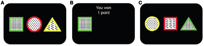
Figure 1. Schematic showing the outline of the task. (A) The subject is presented with three different stimuli. Each stimulus has a different feature along each one of the three feature dimensions (shape, color and texture). (B) The subject chooses one of the stimuli and receives binary reward feedback, either winning one (as in this case) or zero points. (C) After a short delay a new trial begins and the subject is presented with three new stimuli from which to choose.

2.2. Subjects

Thirty-seven subjects (22 females, ages 18–28, mean 21.3 years) recruited from the Princeton community performed 500–1000 trials of the task. Subjects first performed a similar number of trials in a task that was identical but for the fact that changes in the relevant dimension and most rewarding feature were explicitly signaled. For both parts of the experiment, subjects received on-screen instructions informing them that only one of the three dimensions (color, shape, or texture) was relevant to determining the probability of winning a point, that one feature in the relevant dimension will result in rewards more often than the others (the exact probability was not mentioned), and that all rewards were probabilistic (specifically, that “even the best stimulus will sometimes not reward with a point” and vice-versa). They were also instructed to respond quickly (imposed using a 1-s response timeout) and to try to get as many points as possible.

Subjects practiced the task, and were then instructed that throughout the first part they would be informed when the relevant dimension and best feature were changed. Before the start of the second (unsignaled changes) part, they were instructed that changes in the relevant dimension and best feature would no longer be signaled. In this part, subjects were given a break and allowed to rest after completing each quarter of the trials. In each break they were also informed of their cumulative point earnings since the last break, and how that compared to the maximum possible earnings. In neither part were subjects instructed about the rate of change-points or the hazard function.

After performing the second part, some subjects continued to perform another 300 trials of the signaled task inside a magnetic resonance imaging scanner. Subjects were compensated for their time with either $12 (behavior only) or $40 (scanning experiment). All subjects gave informed consent and the study was approved by the Princeton University Institutional Review Board. As we are interested specifically in the interaction between change-point detection and representation learning, here we focus exclusively on data from the unsignaled portion of the experiment (see Gershman et al., 2010, for an analysis of the first part of the experiment).

2.3. Computational Models

We compared two alternative families of models that could potentially explain human performance on this task. The first, based on Bayesian probability theory, makes use of all available information to infer the action that will maximize the probability of obtaining a reward on the next trial. The second focuses on one feature at a time, testing whether it is the correct feature that maximizes reward. This latter set of models is suboptimal in its use of information, and consequently performs less well on the task. However, it is computational much simpler and thus more tractable in an online highly multidimensional setting. By comparing the fits of the two classes of models to subjects’ trial-by-trial behavior, our aim was to determine which model better describes the computations performed by the human brain in such scenarios.

2.3.1. Notation

We begin by defining some notation common to both models. We let the identity of the relevant dimension (shape, color, or texture) on trial t be d and that of the feature, i.e., the specific shape, color, or texture, be f. On any trial, we say that the set of three stimuli are s_t = (s_t(1), s_t(2), s_t(3)). We write c_t ∈ {1, 2, 3} for the subject’s choice on trial t and r_t ∈ {0, 1} for the reward given in response to that choice. We use the notation c_1:t and r_1:t to denote the set of choices and rewards from trial 1 to trial t. For compactness, we define 𝒟_1:t = (c_1:t, r_1:t) as the history of choices and rewards. Finally, ρ_h and ρ_l are the reward probabilities of the high and low rewarding options, respectively.

2.3.2. Bayesian inference models

The Bayesian model uses probabilistic inference to compute the probability distribution over the identity of the rewarding dimension and feature given all past trials, p(d, f | 𝒟_1:t). Using this, it infers the “value” of each stimulus, that is, the probability that choosing the stimulus will lead to reward, p(r_t+1 | 𝒟_1:t, s_t+1(i)). These values drive choices, with higher values corresponding to higher choice probabilities. This model extends a previous model by Gershman et al. (2010) to allow unsignaled changes in the relevant dimension and feature, using methods of Bayesian change-point detection (Adams and MacKay, 2007; Fearnhead and Liu, 2007; Wilson et al., 2010).

Specifically, we are interested in computing the probability of reward for each possible stimulus, s_t+1(i), based on the observed history of choices and rewards 𝒟_1:t. If the identity of the rewarding dimension, d, and feature, f, were known, this computation would be trivial, as we would simply look for presence or absence of the rewarding feature in the stimulus:

When d and f are unknown, as is the case in our experiment, one must marginalize out uncertainty over d and f:

The key, then, is to evaluate p(d, f | 𝒟_1:t). Gershman et al. (2010) showed how to do this exactly in a stationary environment. However, in the current, dynamically changing, task each change-point renders the previous experience irrelevant for determining the currently correct d and f. Thus for unsignaled change-points one must additionally marginalize over all possible change-points and the uncertainty associated with each. To do this efficiently, we follow the approach of Adams and MacKay (2007), and introduce the run-length, l_t – the number of trials since the last change-point. In cases in which change-points render past information truly irrelevant (i.e., they divide the time series into independent epochs called “product partitions”; Barry and Hartigan, 1992), the run-length determines how much past data is relevant to the current inference¹. Thus we can write

By definition, the run-length either increases by one after each trial, in between change-points, or becomes zero at a change-point. Thus we can define the change-point prior, p(l_t+1 | l_t, 𝒟_1:t) as

where h(t, l_t, 𝒟_1:t) is the hazard rate, the prior probability that a change occurs. In general, the hazard rate can vary as a function of time (trial), run-length, and the specifics of the past data. However, many real-world scenarios are not as convoluted. Specifically, for the current task we consider two different versions of the Bayesian model: one in which the hazard rate h is taken to be the true hazard rate from the experiment, i.e., a uniform probability of change between trials 15–25 after the previous change-point (hereafter Bayes var h to denote the variability of the hazard rate as a function of time), and a second slightly simplified model which (incorrectly) assumes a constant hazard rate (hereafter Bayes const h). The former model is motivated by the fact that the subjects have already played 500–1000 trials of the task with signaled changes and thus might reasonably be expected to have learned an approximation to the correct hazard rate. In the latter, approximate model, we fit the constant hazard rate separately to each subject’s behavior (see below). In both models the hazard rate depends, at most, on l_t, hence below we drop the dependences on t and 𝒟_1:t.

Substituting the change-point prior, equation 4, into equation 3 gives

where p(d, f | l_t+1 = 0) is the (uniform) prior probability of d and f after a change-point.

We now need to specify two distributions: (1) p(d, f | l_t+1 = l_t + 1, 𝒟_1:t), which is the probability distribution over the rewarding feature (d,f), conditioned on the run-length l_t+1 = l_t + 1 and past data; and (2) p(l_t | 𝒟_1:t), the inferred distribution over the run-length up to the current trial, given the observed data.

The first of these, p(d, f | l_t+1 = l_t + 1, 𝒟_1:t) can be computed efficiently and recursively using Bayes’ rule

The run-length distribution p(l_t | 𝒟_1:t), can also be computed recursively using Bayes’ rule according to

Taken together, these equations define a Bayesian update process that makes optimal use of past information to infer the present identity of the most rewarding feature with unsignaled change-points.

In order to generate choice probabilities the model looks one time step into the future to compute stimulus values, that is, the predicted reward outcome for each choice V(s_t+1(i)) = p(r_t+1 | 𝒟_1:t, c_t+1 = s_t+1(i)) and then uses a softmax choice function² (also called a Boltzmann distribution) to generate choice probabilities based on these values:

where β is an inverse temperature parameter which will be fit to data. Thus for a given Bayesian model (Bayes const h or Bayes var h) and a set of parameters (β, h, ρ_h, and ρ_l for Bayes const h; β, ρ_h and ρ_l for Bayes var h) this equation allows us to compute the probability of the next choice given previous choices. In section 3.3 we use this to decide which of the models fits the data best.

Note that, unlike the inference process, the decision process is suboptimal. This reflects the fact that although “ideal observer” inference of reward probabilities in this task is tractable, determining the optimal action selection policy while taking account of the multiple levels of uncertainty about these inferences is far from trivial.

Figures 2 and 3 illustrate this algorithm in action. Figure 2 shows the detailed update process for six steps of the model, for simplicity illustrated for the case of no change-points. Figure 3 depicts the evolution of p(d, f | 𝒟_1:t) over a longer time scale that includes unsignaled changes.

FIGURE 2

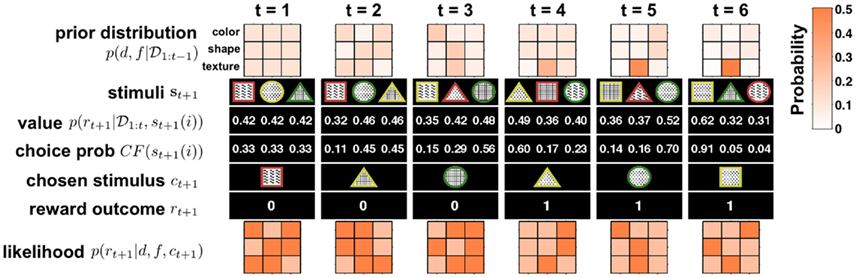
Figure 2. Illustration of six time steps of the Bayesian model in action with no change-points. Starting from t = 1 from top to bottom: the model begins with a uniform prior distribution over dimension d and feature f, p(d, f | 𝒟_1:t) (rows in 3 × 3 plot denote dimensions, with three features each; shading denotes probability; see scale on right). Next the three stimuli, {s}_t+1 = {s_t+1(1), s_t+1(2), s_t+1(3)}, are observed and their values, p(r_t+1 | 𝒟_1:t, s_t+1(i)), computed. Given these values the choice probability CF(s_t+1(i)) is computed for each option (here with β = 10) and a choice c_t+1 is made. After the choice the model receives feedback about the reward, r_t+1, and uses this to compute the likelihood for each dimension and feature pair, p(r_t+1 | d, f, c_t+1), which is equal to either ρ_h or ρ_l. This likelihood is then multiplied by the prior distribution p(d, f | 𝒟_1:t) to obtain (after normalization) the posterior distribution over dimensions and features, which is the new prior distribution at the next time step. As is evident from the figure, on every trial the model gains new information about all the dimensions and features, thus allowing it to rapidly converge on the correct inference n(in this case, that the second texture feature, dots, were the most rewarding).

FIGURE 3

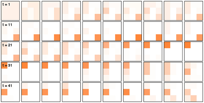
Figure 3. Illustration of the Bayesian model in action with unsignaled change-points. Each square represents p(d, f | 𝒟_1:t), the distribution over correct dimension and feature, at a different trial, starting with trial 1 in the top left and finishing with trial 50 in the bottom right corner. There are two unsignaled change-points in this data set, on trials 15 and 30. The model requires quite a few trials to detect the change (and the resulting drop from 75% chance of reward to 42%), but does so reliably.

2.3.3. Selective attention models

The second family of models assumes that subjects use a simplified “serial-hypothesis-testing” strategy to solve the task. In particular, this model postulates that at each point in time the subject focuses attention on one feature f * of one dimension d*. The subject then chooses the stimulus containing this feature until such time that the subject decides to switch attention to a different dimension and feature. This strategy requires substantially fewer computational resources than the Bayesian inference strategy, however this comes at the price of suboptimal use of information and diminished performance on the task.

We focus on three formal instantiations of the selective attention model. These are by no means the only possibilities within this family of models, but they capture the essential features of selective attention while remaining amenable to analysis.

2.3.3.1 Selective attention with hypothesis testing (SA full). This model performs a Bayesian hypothesis test to determine whether to switch from, or stick with, the currently attended dimension and feature, based on the reward history since switching attention. It shares some similarities with the model of Yu and Dayan (2005), which also entertains only one possibility at a time for the relevant feature, although in their model the dynamics of attention switching are deterministic while in our model they are probabilistic.

The SA full model tracks the probability that the currently attended dimension-feature pair is the most rewarding one based on the history of rewards experienced since the last shift of attention. We write n as the number of time steps since the last shift of attention and p({d*, f *}_t | r_t−n+1:t) as the probability that dimension d* and feature f * are correct at time t given the last n rewards. Using Bayes rule it is then straightforward to show how this probability distribution updates over time

Here p(r_t | {d*, f *}_t) is the probability of seeing reward outcome r_t given that the attended dimension-feature pair is correct, which is just ρ_h if r_t = 1 and (1 − ρ_h) if r_t = 0. Also, if we assume a constant hazard rate for unsignaled changes in the task we have

where U(d*, f *) is a uniform distribution over d* and f *. Taken together this leads to the following recursive update equation for p({d*, f *}_t | r_t−n+1:t)

Similarly, we can compute the probability that the attended dimension-feature pair is not correct, i.e., p(¬{d*, f *}|r_t−n+1:t) = 1 − p({d*, f *}|r_t−n+1:t).

Given these two probabilities, the log likelihood ratio between the hypothesis that the current focus of attention is on the highly rewarding feature, and the alternative hypothesis is

which in turn determines the probability of switching the focus of attention according to

with inverse temperature parameter β and threshold þ as free parameters of the model. Note that this model essentially reduces to leaky counting of the number of wins and losses. An outline of the model in action is shown in Figure 4.

FIGURE 4

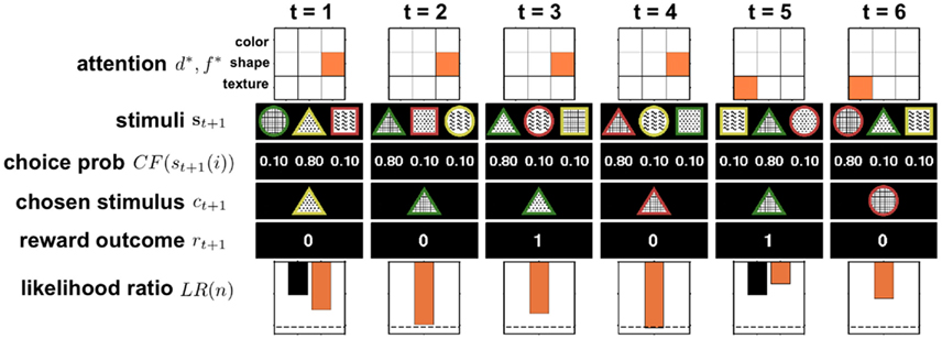
Figure 4. Illustration of six trials of the full selective attention model in action. At t = 1 the model randomly picks one dimension-feature (d*, f *) pair, in this case (shapes, triangle), to attend to. Then the three stimuli {s}_t+1 = {s_t+1(1), s_t+1(2), s_t+1(3)} are observed and ε-greedy choice probabilities are computed (in this example ε = 0.3). Next a stimulus is chosen, c_t+1, and the reward outcome, r_t+1, observed. The observed reward is used to update the log likelihood ratio LR(n). For clarity, the black bar indicates the initial log likelihood ratio and the orange bar represents the updated log likelihood ratio that takes into account the new reward value. If the log likelihood ratio crosses the threshold (dashed line), as occurs here on trial 4, the agent switches its attention randomly (in this case, to (textures, plaid)) and resets its log likelihood ratio to the initial value (black bar at trial 5).

2.3.3.2 Selective attention with win-stay-lose-shift style switching (SA WSLS). We also considered two simplified versions of the selective attention model. In the first, we assume that the subject shifts attention with probability g_win if the last trial was rewarded with a point or g_loss if it was not rewarded. This model performs the task at better than chance levels as it is less likely to switch away from the correct (often rewarded) dimension-feature pair.

2.3.3.3 Selective attention with random switching (SA rand). In this second, simplest possible, selective attention model, we assume that subjects switch the focus of their attention randomly with some fixed probability g, regardless of reward feedback. We further assume that the subjects are memoryless such that they are equally likely to switch their attention to any of the possible dimensions and features (including the last focus of attention). It is important to note that, when simulated, this model cannot actually perform the task at above-chance levels since switching is unrelated to the reward outcomes. Nevertheless, when used as a tool to infer the subjects’ center of attention from the data, this model can be useful as an approximation to the more complex selective attention models as it captures a key feature of selective attention choice behavior, i.e., that choices are correlated across trials such that the subject tends to choose a certain feature in a certain dimension for a length of time.

2.3.3.4 Choice probabilities. We use an ε-greedy policy for all selective attention models, such that the agent picks the option with the attended feature with probability 1 − ε, and chooses randomly with probability ε. Such a choice rule allows for mistakes, that is, trials in which an option that does not have the attended feature is chosen by accident. In these trials, the current value of LR(n) is not changed. Note that the ε-greedy choice function used here is similar to a softmax choice function (as used in the Bayesian models) if one assumes that a selective attention agent attaches higher value to a stimulus with the attended feature, than to other stimuli.

2.3.3.5 Inferring the attended feature. While these selective attention models provide straightforward accounts of the generation of subjects’ choices, it is complicated to fit them to subjects’ behavior. This is due to an additional source of uncertainty: the experimenter’s uncertainty about the subject’s focus of attention on each trial. For example, it is impossible to conclude, only on the basis of the observation that the subject has chosen a red-plaid-circle stimulus, which of the three features (red, plaids, or circles) was the focus of attention. We can only infer a distribution over the target feature given the subjects’ choice and reward history, p(d*, f * | 𝒟_1:t). Using this, we can compute the likelihood of choosing each option according to

where p(s_t+1(i) | d*, f *) is determined by the ε-greedy choice function as follows

To compute the probability that a feature is attended to, p(d*, f * | 𝒟_1:t), we again use the change-point algorithm of Adams and MacKay (2007), with change-points now reflecting the subject’s switches in attention, rather than the dynamics of the task:

Here, we introduce as the run-length since the last time the attentional focus was shifted (as distinct from l_t in the Bayesian model which denotes the run-length since the last change-point in the task). As before, can be computed recursively via

and

The exact form of the change-point prior, depends on the selective attention model:

Finally, we assume a uniform distribution over d* and f * as the initial condition.

As was the case for the Bayesian model, computing p(c_t+1 | 𝒟_1:t), the probability of the next choice, given the parameters of each model and past choices, allows us to compare the different models’ abilities to fit the observed behavioral data.

2.4. Model fitting and model comparison

To adjudicate between the models, we used human trial-by-trial choice behavior to fit the free parameters ω_m of each model m, and asked to what extent each of the models explains the subjects’ choices.

The free parameters, ω_m for each model are shown in Table 1. Model likelihoods were based on assigning probabilities to the individual choices of each subject, according to equation 8 for the Bayesian models and equation 14 for the selective attention models, such that the likelihood of the choices given model m and parameters ω_m was given by

TABLE 1

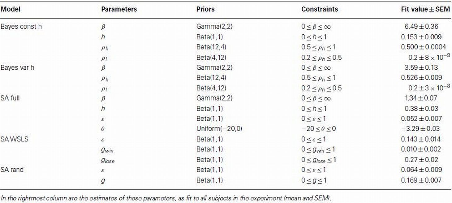
Table 1. List of parameters with accompanying priors and constraints used in the model-based analysis.

We fit each model’s parameters to each subject’s data separately. To facilitate this, we used regularizing priors that favored realistic values and maximum a posteriori (MAP; rather than maximum likelihood) fitting (Daw, 2011). These priors and constraints are summarized in Table 1 along with the mean fit values for each of these parameters.

We optimized model parameters by minimizing the negative log posterior of the data given different settings of the model parameters using the Matlab function fmincon. The best fitting parameters for each model were then used to compute the Laplace approximation to the Bayesian evidence E_m for each model (Kass and Raftery, 1995):

in which is the value of the prior on the parameters at the MAP estimate, is the data likelihood at the MAP estimate, G_m is the number of parameters in model m and |H_m| is the determinant of the Hessian matrix of second derivatives of the negative log posterior evaluated at the MAP estimate. The Bayesian evidence is a means for comparing different models and correctly penalizing those with large number of free parameters. As the Bayesian evidence scales with the number of data points and thus can be hard to interpret, we computed an average probability per trial for each model by dividing the total Bayesian evidence by the number of trials and exponentiating it, i.e.,

The resulting measure, ℘_m, retains many of the useful features of the evidence, E_m, such as including correction terms that take account of the number of free parameters in a model, while also being a more intuitive measure of variance explained by the model. In particular, ℘_m varies between 0 and 1, with ℘_m = 1/3 approximating chance choice probabilities in our model (indicating that the model does not explain any variance in the data, or alternatively, that the data provide no support for the model), while ℘_m = 1 implies that a model predicts the observed choices perfectly. More generally, in cases where the Laplace approximation to E_m is valid (Kass and Raftery, 1995), ℘_m can be shown to approximate the geometric mean of the choice probabilities given the maximum likelihood parameter settings of the model,

3. Results

We first describe the qualitative features of subjects’ behavior on our task, before presenting more detailed analyses to determine n which model explains better subjects’ choices. We use two types of analyses: in a qualitative analysis, we test the data for distinctive patterns that are predicted by each of the models. In the second, quantitative analysis, we use the whole sequence of trial-by-trial choices and rewards in order to fit each of the models, and compare the likelihoods of the data given each model while accounting for their different numbers of free parameters. The results of both of these analyses indicate that the selective attention class of models better explains subjects’ behavior in our task.

3.1. Learning Curves

Figure 5A shows performance (fraction correct choices) as a function of the number of trials after an unsignaled change-point, averaged over all subjects. From this learning curve it is apparent that subjects were able to learn the correct dimension and feature, and in general to perform the task at better than chance levels, despite its difficulty. Furthermore, performance did not deviate from chance for several trials after a change in the correct dimension and feature occurred, suggesting that it takes several trials for subjects to detect and respond to the change.

FIGURE 5

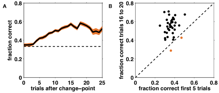
Figure 5. Performance on the task as a function of number of trials after an unsignaled change-point. (A) Fraction correct choices as a function of trial number after a change-point, averaged across subjects (solid black line). Shading – SEM; dashed line – chance responding. (B) Comparison of average performance on trials 1–5 after a change and trials 16–20 after a change for each individual subject. The dashed black line corresponds to equality such that subjects lying above this line improved their performance over the course of a block. The two subjects that did not meet this criterion are shown in orange.

To assess each subject’s degree of learning we compared the average fraction correct on the first five trials after a change to the average fraction correct on trials 16–20 after the change (providing that another change has not yet occurred). This is depicted in Figure 5B. Points above the equality line indicate subjects whose performance improved between change-points. In the rest of the analyses we focus on the 35 (out of 37) subjects who showed such improvement.

3.2. Qualitative Analysis

The main qualitative difference between the two classes of models we propose is that a Bayesian learner learns about all features of the chosen stimulus, whereas a selective attention learner only learns about one feature in each trial. Thus the selective attention model predicts that if a subject switches the focus of attention after a zero-reward trial, she is equally likely to switch to any feature, including the unattended features of the recently chosen (and unrewarded) stimulus. In contrast, the Bayesian model, having associated all the features of the last choice with the zero point outcome, is likely to avoid all of these features in the next choice, to the extent that this is possible.

Unfortunately, as discussed above, we cannot directly infer the focus of attention from a single choice in our task. However, we can glean some information about the focus of attention in a model-free way from pairs of consecutive trials in which only one feature is common to both choices. On this subset of trials, for the selective attention model, there is a high probability that the currently attended feature is the feature common to both choices. We can then ask what happens on the next trial (i.e., the third trial in the sequence), based on the history of rewards for the first two trials, i.e., whether the two previous trials were “loss” trials (denoted as 00) or “win” trials (11). Specifically, we asked whether the third choice shared the putative attended feature (“stick”) or not (“switch”), and whether it included 0, 1, or 2 of the previous putatively unattended features. For instance, based on two consecutive trials in which a red-plaid-square and a red-dots-triangle were chosen, we guess that “red” was the attended feature, and ask: if both trials resulted in 0 reward, will the subject “stick” with red on the third trial? And if not, will the subject also tend to avoid dots and triangles (as predicted by the Bayesian class of models, but not the selective attention models)?

Figure 6 compares the behavior of subjects (Figures 6E,F) with that of 100 simulations of one model from each class (Bayes const h, Figures 6A,B, and SA full, Figures 6C,D; these were the models in each class found to best fit the behavioral data, see below). The left column (Figures 6A,C,E) shows the frequency of switch and stick trials for the two different reward conditions. As expected, the behavior of both models is qualitatively similar and very close to that of the subjects. The right column (Figures 6B,D,F) shows the distribution over the number of shared features on the unattended dimension. Figure 6B clearly shows that the Bayesian model seeks to avoid all features paired with a loss, as the distribution over the number of shared features is shifted to the left for loss trials as compared to win trials. The selective attention model (Figure 6D), however, shows no such difference between loss and win trials. Importantly, the predictions of the selective attention model are in line with the behavior of the subjects (Figure 6F).

FIGURE 6

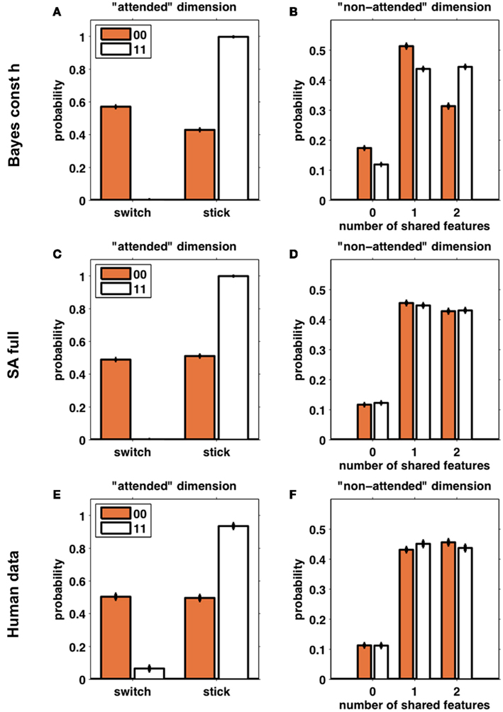
Figure 6. Simulated data from the Bayes const h model (A,B) and SA full model (C,D) (100 “subjects” simulated for each model) compared with human behavior (E,F). Left column (A,C,E): the probability of switching away from the putatively attended dimension based on whether the outcomes for the last two trials were two losses (orange) or two wins (white). Right column (B,D,F): the number of shared features between the third choice and the second choice, in the putatively unattended dimensions, divided according to the outcomes of the last two trials (orange – two losses; white – two wins). Error bars are SEM.

3.3. Quantitative Model Comparison

3.3.1. Model evidence and choice probabilities

Figure 7A shows the average probability per choice ℘_m (see section 2.4) for each of the five models, averaged across subjects. All of the models perform better than chance, with the full selective attention model explaining the data best. A more detailed view of this result is shown in Figure 7B which plots histograms of the choice probabilities for the five different models, pooled across subjects. This demonstrates that the full selective attention model predicts more choices with high probability than any of the other models. Figure 8 further confirms this population-level trend at the single subject level. Here we compared ℘_m for each model against the full selective attention model. For all four other models, the full selective attention models better explained the data in a majority of subjects³.

FIGURE 7

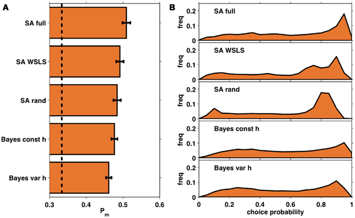
Figure 7. (A) Average choice probabilities, ℘_m, for each of the five models averaged across subjects. Dashed line: chance; error bars: SEM. (B) Histograms of choice probabilities for the five different models using data from all 35 subjects.

FIGURE 8

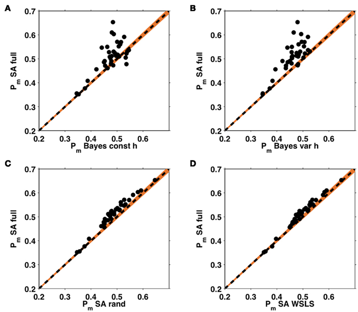
Figure 8. Within subject analysis of average choice probabilities. ℘_m values from the full selective attention model plotted against those of the four other models: the Bayesian model with constant (A) and variable (B) hazard rates, and the selective attention models with random (C) and win-stay-lose-shift (D) switching. Each dot represents an individual subject, the black dashed line indicates equality, such that the choices of any subject lying above this line are better explained by the full selective attention model. Orange shading represents a confidence interval outside which the Bayesian evidence favors one model over the other with p < 0.0001.

3.3.2. Confusion matrix

We assessed the sensitivity of our analysis by asking to what extent our model fitting procedure was able to correctly recover the identity of a model from simulated data. Specifically, we used each model to simulate 200 subjects (500 trials each), using parameter values consistent with the values fit to subjects’ behavior (that is, parameter values drawn from empirical priors generated from the above fits to subjects’ choice data). We then fit each of the five models to each simulated subject, and determined the model that best fit the subject’s data.

The results of this analysis are summarized in the “confusion matrix” (Steyvers et al., 2009) shown in Figure 9. Numbers in each box correspond to the percentage of simulations for which the model on the x-axis provided the best fit to data generated by the model on the y-axis. If our ability to recover the model that generated the data was perfect, this matrix would be zero everywhere except on the diagonal where it would have value 100. Unfortunately, some of the models we tested predict sufficiently similar behavior on this task, such that there are significant off-diagonal elements in this matrix. However, reassuringly, for all models the correct model is identified as best explaining the data most often, and, importantly, there is very little mixing between models in the two different (selective attention and Bayesian) classes. This further validates our results supporting the selective attention class of models.

FIGURE 9

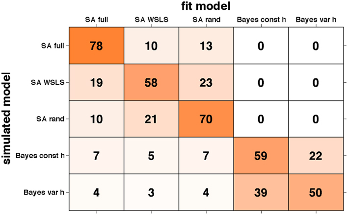
Figure 9. Confusion matrix showing the percentage of times data generated by the model on the y-axis was fit by the model on the x-axis. Shading corresponds to the numbers such that darker represents higher numbers.

3.3.3. Model learning curves

Although the above analysis of choice behavior strongly favors the selective attention model, it is important to ask whether an independent agent playing that strategy can perform the task at a level comparable with that of humans. To test this, we simulated two agents – one playing according to the Bayesian model with fixed hazard rate and the other using the full selective attention strategy, with optimal parameter settings – and measured their learning curves.

In the Bayesian case, the optimal parameters correspond to a deterministic choice function (β = ∞) and a hazard rate set as the average hazard rate for the task (h = 0.05). In the selective attention case, we assumed that optimal behavior has zero decision noise, ε = 0, and searched the parameter space to find optimal values for the other three free parameters, resulting in β = 50, þeta = −2.1984, h = 0.0333. With these parameter settings, we simulated 100,000 trials for each model and computed average learning curves as shown in Figure 10. Clearly, both agents can perform the task, but with very different degrees of success. Performance of the Bayesian model far outstrips that of both the selective attention model and the human subjects, as might be expected from a model that makes near optimal use of information. The selective attention model, however, performs similarly to (but marginally worse than) the human subjects.

FIGURE 10

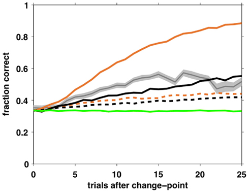
Figure 10. Average learning curves for simulated agents performing 10,000 trials of the task with unsignaled changes. Black – full selective attention model with optimal (solid) and fit (dashed) parameters; Orange – Bayesian model with constant hazard rate with optimal (solid) and fit (dashed) parameters; Green – SA rand with fit parameter values; Gray – human data (shading: SEM).

One possible reason for the inferior performance of the selective attention model compared to human subjects is that we modeled a memoryless selective attention model (for reasons of tractability of the model-based choice analysis). Thus, our selective attention agent has a probability of 1/9 of switching to the same feature once it decides to switch its focus of attention, while humans presumably always switch to a different feature.

For comparison, we also simulated the Bayesian, full and random selective attention agents using parameter values found using the fitting procedure. As expected from a model that pays no attention to rewards, the SA rand model shows no learning and performs at chance levels throughout. Both the Bayesian and SA full models have learning curves with fit parameters that are shallower than human behavior.

4. Discussion

Much progress has been made in recent years in understanding how humans and animals learn to maximize rewards by trial and error. However, this work has often eschewed the question of how the representation on which this learning process relies, is itself learned. We investigated this “representation learning” process in a task in which humans had to learn concurrently which of three dimensions is relevant to rewards, and within this dimension, which feature is associated with the highest probability of reward. To exacerbate uncertainty in the task and further mimic learning in real-world scenarios, the underlying reward-generating process changed abruptly at different time points, unannounced to the subjects. Thus our task involved uncertainty at multiple levels: uncertain representations, uncertain (probabilistic) rewards and uncertainty regarding change-point locations.

4.1. Subjects are Suboptimal

Surprisingly, in contrast to perceptual decision making tasks in which humans are often shown to be Bayes-optimal evidence integrators (Ernst and Banks, 2002; Alais and Burr, 2004; Kording and Wolpert, 2004), our analysis provides strong evidence that subjects in our task use evidence suboptimally. Rather than estimating a probability distribution over the identity of the rewarding dimension and feature, our subjects’ performance was more consistent with a “selective attention” serial-hypothesis-testing strategy in which the subject attends to one feature at a time, accumulating information about the likelihood that this feature is the most rewarding one.

There are at least two possible explanations for this suboptimality. The first is that subjects in our task are less trained compared to many of the human and animal subjects used in psychophysical and perceptual tasks. Thus they may have not yet learned the correct Bayesian strategy. While this may account for differences from experiments such as (Munuera et al., 2009) that investigated sensorimotor integration in humans (which can be assumed to be highly trained from everyday experience), it is hard to see how the subjects in an experiment such as (Bahrami et al., 2010) would be significantly more trained than our subjects.

Instead, we conjecture that there is a more general reason for subjects’ suboptimal representation learning: optimal performance in our task requires significantly more computational capacity than needed to optimally solve any of the referenced perceptual tasks. Specifically, implementing the full Bayesian model with a variable hazard rate involves keeping track of up to 300 probability values (30 weights for each possible run-length plus 30 nine-valued probability distributions p(d, f | l_t, 𝒟_1:t) for each possible run-length). This is considerably reduced in the fixed hazard rate case, to 9 values, but even this is more complicated than in the referenced papers.

In contrast, the selective attention model demands far fewer computational resources, requiring the maintenance of only two variables, the identity of the attended feature and the likelihood ratio, at any time step. This process is not wholly computationally suboptimal, as it at least utilizes an optimal (Bayesian) computation of the likelihood that the currently attended feature is the most rewarding. However, since this strategy does not take all available information into account, learning is slower in terms of the amount of experience that is needed in order to learn the correct representation.

Such an account may explain why in a related, but simpler, task with only two dimensions and features (Wunderlich et al., 2011) the authors found evidence for Bayesian learning over a model that selectively attended to the dimensions (although their selective attention model was different from the one presented here in that it attended to dimensions rather than features). It is possible that humans have the computational capacity to integrate information optimally in relatively simple tasks but switch to simpler strategies as task difficulty increases.

In real-world representation learning in which the number of possible relevant dimensions and features is potentially huge, we expect the difference in computational efficiency between selective attention and fully Bayesian strategies to be even more pronounced. Thus we conjecture that it is impossible for humans to implement a full Bayesian solution in the real-world and thus, even in our relatively simple task, they are using an alternative approximate mechanism which is computationally efficient but statistically suboptimal (see also Steyvers et al., 2003).

4.2. Limitations of the Experiment and Analysis

The main limitation of the current experimental design was that we could not directly measure the subjects’ focus of attention. To nevertheless estimate choice probabilities for the selective attention models, we used the subjects’ sequence of behavioral choices and outcomes to infer the dynamically changing focus of attention. On some trials this method has significant uncertainty about the focus of attention, which reduces the power of our statistics in differentiating between models. Still, our results supported the selective attention models unambiguously. In future work we hope to overcome this limitation using modified versions of the task.

Another limitation is that our current analysis does not include a selective attention model with memory for options that have already been tested. This is because exact inference in change-point problems is intractable when data are correlated across change-points (as would be the case across attentional switches in such a model). In future work we will examine the possibility of performing approximate inference in these cases.

4.3. Relation to Prior Work on Selective Attention

The two families of models that we explored, Bayesian and selective attention models, can be thought of as formal instantiations of previous models of discrimination learning: the Bayesian model expounding the “continuity theory” of early behaviorists (reviewed in Mackintosh, 1965), in which all sensory dimensions and features are treated equally in learning, and the selective attention family formalizing “non-continuity theory” (Lashley, 1929; Krechevsky, 1938), which in its strongest form proposes that animals only learn about the features they attend to.

Our results favor the latter theory. Because we have a precise formulation of the models in both cases, we can, in line with early theories of selective attention (Broadbent, 1958; Kahneman, 1973; Bundesen, 1996), conjecture that selective attention is favored for reasons of computational efficiency. This interpretation is distinct from (and orthogonal to) the Bayesian models of selective attention from Dayan et al. (2000), in which dynamical allocation of attention arises naturally as a result of Bayesian computations and is not driven by computational costs.

However, prior work also suggests models that we have yet to explore. Specifically, many past studies have found evidence for two-stage models of selective attention (Sutherland and Mackintosh, 1964). In these hierarchical models, an attentional spotlight highlights one particular feature or dimension at the lower level, while a higher-level meta-decision about where to switch attention to is driven by all available information (perhaps weighted by the attentional spotlight).

In this light, Dehaene and Changeux’s (1991) cognitive models of the Wisconsin card sorting task suggest several possible hierarchical extensions to our model. Two, in particular, are of interest here. The first extends the present selective attention model by including memory – assuming that hypotheses that have been ruled out are not immediately revisited. The second assumes that subjects use some sort of reasoning to allocate the attentional spotlight, rather than selecting their next focus of attention randomly. In our case, this latter model would amount to a mixture of the Bayesian and selective attention models in which a Bayesian high-level analysis directs the focus of attention (biasing it toward features likely to be rewarding) while the attentional model performs hypothesis testing to determine whether the currently attended feature is indeed more rewarding.

Unfortunately, an exact model-based analysis is not possible in these cases due to violation of the product partition assumption. More work employing approximate inference schemes and different experimental manipulations will be needed to distinguish between these more subtle instantiations of selective attention.

The full selective attention model shares many similarities with that of Yu and Dayan (2005). In their model of an extended Posner task, the agent focuses on one relevant feature at a time and performs an approximate likelihood ratio test to decide when to switch the center of attention. Unlike our model, attention switches are deterministic, and the new center of attention is not determined immediately after a switch but after ten passive “null trials.” While such a strategy is likely to work in a detection task like the Posner task, in a task such as ours in which subjects must make active choices it seems unlikely that such a passive strategy would work.

Despite these differences, it is interesting to speculate whether the attention switching mechanism, proposed by Yu and Dayan (2005) to be driven by acetylcholine and norepinephrine, is used in our task. In particular, this would map the likelihood ratio in equation 12 onto the activity in these two systems with norepinephrine encoding the probability that the currently attended feature is incorrect p(({d*, f *} | r_t−n+1:t) (the so-called “unexpected uncertainty”) and acetylcholine encoding ρ_h, the probability of winning given that the currently attended feature is correct (“expected uncertainty”).

5. Conclusion

We have presented a novel experimental paradigm in which humans infer the relevance of different features of stimuli to determining rewards, in a changing environment. Analysis of choice behavior in this task suggests that humans use a suboptimal inference process based on a selective attention serial-hypothesis-testing strategy in which subjects focus on just one feature of the stimuli at a time. This glaring suboptimality is perhaps justified by the intractability and complexity of the problem at hand – and humans’ extraordinary success at learning new tasks in a highly multidimensional and changing environments attests to its obvious utility.

Conflict of Interest Statement

The authors declare that the research was conducted in the absence of any commercial or financial relationships that could be construed as a potential conflict of interest.

Acknowledgments

We thank S. J. Gershman and M. T. Todd for helpful comments on this work. This research was funded by a Sloan Fellowship (Yael Niv), the Binational United States-Israel Science Foundation and Award Number R03DA029073 from the National Institute on Drug Abuse. The content is solely the responsibility of the authors and does not represent the official views of any of the funders.

Footnotes

1. ^Note that the “product partition” simplification does not strictly hold for our task because here a change was always to a different dimension (e.g., if the relevant feature was red, it could change to waves, but never to green), which means that the data are weakly correlated across a change-point. Nevertheless, we use this approximation as it simplifies inference considerably while making the model only slightly suboptimal in terms of performance on the task.
2. ^It is also possible to use the so-called ε-greedy choice function with this model. In this case, the model chooses the highest value option with probability 1 − ε for some small ε (0 ≤ ε ≤ 1) otherwise choosing randomly between the three options. Empirically, we found this model to fit the data particularly poorly and hence we do not consider it further in this paper.
3. ^Note that the shaded significance region was computed conservatively, according to the subject with the fewest number of trials. For subjects with larger number of trials the shaded region should be smaller.

References

Adams, R. P., and MacKay, D. J. (2007). Bayesian Online Changepoint Detection. Cambridge: University of Cambridge.

Alais, D., and Burr, D. (2004). The ventriloquist effect results from near-optimal bimodal integration. Curr. Biol. 14, 257–262.

Pubmed Abstract | Pubmed Full Text | CrossRef Full Text

Bahrami, B., Olsen, K., Latham, P. E., Roepstorff, A., Rees, G., and Frith, C. D. (2010). Optimally interacting minds. Science 329, 1081–1085.

Pubmed Abstract | Pubmed Full Text | CrossRef Full Text

Barry, D., and Hartigan, J. A. (1992). Product partition models for change point problems. Ann. Stat. 20, 260–279.

CrossRef Full Text

Behrens, T. E. J., Woolrich, M. W., Walton, M. E., and Rushworth, M. F. S. (2007). Learning the value of information in an uncertain world. Nat. Neurosci. 10, 1214–1221.

Pubmed Abstract | Pubmed Full Text | CrossRef Full Text

Braun, D. A., Mehring, C., and Wolpert, D. M. (2010). Structure learning in action. Behav. Brain Res. 206, 157–165.

Pubmed Abstract | Pubmed Full Text | CrossRef Full Text

Broadbent, D. (1958). Perception and Communication. Elmsford, NY: Pergamon.

Brown, S. D., and Steyvers, M. (2009). Detecting and predicting changes. Cogn. Psychol. 58, 49–67.

Pubmed Abstract | Pubmed Full Text | CrossRef Full Text

Bundesen, C. (1996). Converging Operations in the Study of Visual Selective Attention. Washington, DC: American Psychological Association.

Daw, N. D. (2011). “Trial by trial data analysis using computational models,” in Decision Making, Affect, and Learning: Attention and Performance XXIII, eds M. R. Delgado, E. A. Phelps, and T. W. Robbins (Oxford: Oxford University Press), 3–48.

Daw, N. D., and Courville, A. C. (2007). The pigeon as particle filter. Adv. Neural Inf. Process. Syst. 20, 369–376.

Dayan, P., Kakade, S., and Montague, P. R. (2000). Learning and selective attention. Nat. Neurosci. 3, 1218–1223.

Pubmed Abstract | Pubmed Full Text | CrossRef Full Text

Dehaene, S., and Changeux, J. P. (1991). The Wisconsin card sorting test: theoretical analysis and modeling in a neuronal network. Cereb. Cortex 1, 62–79.

Pubmed Abstract | Pubmed Full Text | CrossRef Full Text

Ernst, M. O., and Banks, M. S. (2002). Humans integrate visual and haptic information in a statistically optimal fashion. Nature 415, 429–433.

Pubmed Abstract | Pubmed Full Text | CrossRef Full Text

Fearnhead, P., and Liu, Z. (2007). On-line inference for multiple changepoint problems. J. R. Stat. Soc. Series B Stat. Methodol. 69, 589–605.

CrossRef Full Text

Gershman, S. J., Cohen, J. D., and Niv, Y. (2010). “Learning to selectively attend,” in 32nd Annual Conference of the Cognitive Science Society, Portland.

Kahneman, D. (1973). Attention and Effort. Englewood Cliffs, NJ: Prentice-Hall.

Kass, R., and Raftery, A. (1995). Bayes factors. J. Am. Stat. Assoc. 90, 773–795.

CrossRef Full Text

Kemp, C., and Tenenbaum, J. B. (2009). Structured statistical models of inductive reasoning. Psychol. Rev. 116, 20–58.

Pubmed Abstract | Pubmed Full Text | CrossRef Full Text

Kording, K. P., and Wolpert, D. M. (2004). Bayesian integration in sensorimotor learning. Nature 427, 244–247.

Pubmed Abstract | Pubmed Full Text | CrossRef Full Text

Krechevsky, I. (1938). A study of the continuity of the problem-solving process. Psychol. Rev. 45, 107–133.

CrossRef Full Text

Lashley, K. (1929). Brain Mechanisms and Intelligence. Chicago: University of Chicago Press.

Mackintosh, N. (1965). Selective attention in animal discrimination learning. Psychol. Bull. 64, 124–150.

Pubmed Abstract | Pubmed Full Text | CrossRef Full Text

Milner, B. (1953). Effects of different brain lesions on card sorting. Arch. Neurol. 9, 100–110.

Munuera, J., Morel, P., Duhamel, J. R., and Deneve, S. (2009). Optimal sensorimotor control in eye movement sequences. J. Neurosci. 29, 3026–3035.

Pubmed Abstract | Pubmed Full Text | CrossRef Full Text

Nassar, M. R., Wilson, R. C., Heasly, B., and Gold, J. I. (2010). An approximately Bayesian delta-rule model explains the dynamics of belief updating in a changing environment. J. Neurosci. 30, 12366–12378.

Pubmed Abstract | Pubmed Full Text | CrossRef Full Text

Niv, Y. (2009). Reinforcement learning in the brain. J. Math. Psychol. 53, 139–154.

CrossRef Full Text

Steyvers, M., Lee, M. D., and Wagenmakers, E. J. (2009). A Bayesian analysis of human decision-making on bandit problems. J. Math. Psychol. 53, 168–179.

CrossRef Full Text

Steyvers, M., Tenenbaum, J. B., Wagenmakers, E. J., and Blum, B. (2003). Humans use approximate (rather than optimal) Bayesian inference even in relatively simple scenarios. Cogn. Sci. 27, 453–489.

CrossRef Full Text

Sutherland, N. S., and Mackintosh, J. (1964). Discrimination learning: non-additivity of cues. Nature 201, 528–530.

Pubmed Abstract | Pubmed Full Text | CrossRef Full Text

Sutton, R. S., and Barto, A. G. (1990). “Time-derivative models of pavlovian reinforcement,” in Learning and Computational Neuroscience: Foundations of Adaptive Networks, eds M. Gabriel, and J. Moore (Cambridge: MIT Press), 497–537.

Sutton, R. S., and Barto, A. G. (1998). Reinforcement Learning: An Introduction. Cambridge: MIT Press.

Wilder, M., Jones, M., and Mozer, M. (2009). “Sequential effects reflect parallel learning of multiple environmental regularities,” in Advances in Neural Information Processing System, Vol. 22, eds Y. Bengio, D. Schuurmans, J. Lafferty, C. K. I. Williams, and A. Culotta (Cambridge: MIT Press), 2053–2061.

Wilson, R. C., Nassar, M. R., and Gold, J. I. (2010). Bayesian online learning of the hazard rate in change-point problems. Neural Comput. 22, 2452–2476.

Pubmed Abstract | Pubmed Full Text | CrossRef Full Text

Wunderlich, K., Beierholm, U. R., Bossaerts, P., and O’Doherty, J. P. (2011). The human prefrontal cortex mediates integration of potential causes behind observed outcomes. J. Neurophysiol. 106, 1558–1569.

Pubmed Abstract | Pubmed Full Text | CrossRef Full Text

Yu, A. J., and Cohen, J. D. (2009). “Sequential effects: superstition or rational behavior?” in Advances in Neural Information Processing Systems, Vol. 21, eds D. Koller, D. Schuurmans, Y. Bengio, and L. Bottou (Cambridge: MIT Press), 1873–1880

Yu, A. J., and Dayan, P. (2005). Uncertainty, neuromodulation, and attention. Neuron 46, 681–692.

Pubmed Abstract | Pubmed Full Text | CrossRef Full Text