Computational model of precision grip in Parkinson's disease: a utility based approach

Introduction

Precision grip (PG) is the ability to grip objects between the fore-finger and thumb (Napier, 1956). Successful performance of PG requires a delicate control of two forces (grip force, F_G, and lift force, F_L) exerted by two fingers on the object. In a grip-lift task F_G is kept sufficiently high to couple F_L with the object via the agency of friction between the object and the fingers. An optimal F_L is also required to overcome the object's weight and lift it off the surface of the table on which it rests. These forces (F_L and F_G) are thought to be generated in parallel by different subsystems in the brain (Ehrsson et al., 2001, 2003). The critical F_Gat which the object slips is called the slip force (F_slip) and the difference between the actual steady state F_G(SGF), used in a successful lift, and F_slip is known as the safety margin (SM = SGF − F_slip). Johansson and Westling (1988) demonstrated the SM in controls to be 40–50% of slip force (Johansson and Westling, 1988). A high SM is employed to prevent the object from slipping due to internal (accelerations due to arm motion) (Werremeyer and Cole, 1997) and external (random changes in object load) perturbations (Eliasson et al., 1995)—motor activity is optimized for the internal perturbations and this optimality is lost on the addition of an external perturbation external perturbation (Charlesworth et al., 2011; Sober and Brainard, 2012; Wolpert and Landy, 2012). An excessive SM is undesirable as it would cause muscle fatigue and may even lead to crushing of the object.

SM in grip force is a crucial and defining parameter of PG performance. F_slip serves as the threshold below which the object cannot be lifted. Human subjects operate at F_G that is much higher than F_slip; operation at a small SM makes the gripping unstable. Therefore, this need to operate sufficiently far from the border of instability may be regarded as a strategy for minimizing risk. The need for a large SM indicates that concepts from theories of risk-dependent decision making (DM) may be applied to understand PG performance (Bell, 1995; D'Acremont et al., 2009). By definition, risk is the variance in reward outcome (Bell, 1995; D'Acremont et al., 2009). In the context of PG performance, a reward may be thought to be associated with successful lifts. The risk is maximum close to F_slip and expected reward (value) saturates for grip forces much greater than F_slip. Optimal PG consists of maximizing average reward while minimizing risk. The present study approaches the problem of PG in terms of risk minimization and describes it within the framework of Reinforcement Learning (RL). The model is used to explain PG performance in both controls and Parkinson's disease (PD) patients.

PG studies in PD patients show a remarkable difference in SM patterns between PD patients and controls (Ingvarsson et al., 1997; Fellows et al., 1998). PD patients were shown to be capable of storing and recalling previous lift parameters (Muller and Abbs, 1990; Ehrsson et al., 2003). This allows them to scale F_G when the load force on the object changes (Gordon et al., 1997; Fellows et al., 1998). Interestingly, even though F_G scaling is preserved, scientific community is divided on the question of sensory deficits in PD patients being a cause for their altered SM. A sensory deficit would lead to suboptimal sensory-motor coordination. Some studies support the above theory of sensory deficit in PD (Moore, 1987; Schneider et al., 1987; Klockgether et al., 1995; Jobst et al., 1997; Nolano et al., 2008) and others (Gordon et al., 1997; Ingvarsson et al., 1997) reject it. Ingvarsson et al. (1997) demonstrated that the controls and PD OFF patients generated nearly similar SGFs. A higher SGF was generated in PD ON (L-Dopa Medication) case when the lifted object was covered with silk, suggesting a higher safety margin in PD ON condition (Ingvarsson et al., 1997). It has been suggested that this increase in SGF may be due to L-Dopa induced hyperkinesias (Ingvarsson et al., 1997; Gordon and Reilmann, 1999). In another study, Fellows et al. (1998) observed that PD ON subjects show a higher SGF than controls, but there was no mention of PD OFF results (Fellows et al., 1998). Reports also suggest a considerably higher SGF variance in PD OFF condition when compared to controls and PD ON condition (Ingvarsson et al., 1997). This may indicate the importance of the concepts of risk sensitivity in understanding the SGF in controls, PD ON and PD OFF conditions. Furthermore, recent evidence suggests that risk-takers are less prone to Parkinson's disease (Sullivan et al., 2012). PD medications such as L-Dopa (Ehrsson et al., 2003) and dopamine agonists (Claassen et al., 2011) increase impulsivity and risk-seeking behavior in PD patients. PD subjects under medication tend to show less sensitivity to negative outcomes and therefore tend to make risky choices (Wu et al., 2009). The effect of PD medication (dopamine agonist) in enhancing risk-seeking tendency was also confirmed using the Balloon Analog Risk Task—an elegant assay for risk-related behavior (Claassen et al., 2011). The impairment of risk-processing in PD patients (Ehrsson et al., 2003; Wu et al., 2009; Claassen et al., 2011), and altered SM in PD, makes a risk-based motor control approach to PG performance even more compelling.

None of the previously explained computational models for PG lift tasks (Kim and Inooka, 1994; Fagergren et al., 2003; de Gruijl et al., 2009) explain the grip force levels used by controls and PD patients. Hence, a computational model to explain grip forces in controls and PD forms the motivation for the present work.

Drawing from the aforementioned presentation of facts, we propose to model PG performance, and its alterations in PD condition, using the mathematics of risk. We use the concept of utility function, a combination of value and risk components, embedded in the framework of Reinforcement Learning (RL) (Bell, 1995; Long et al., 2009; Wu et al., 2009; Wolpert and Landy, 2012). Concepts from RL have been used extensively in the past to model the function of the Basal Ganglia (BG) in control and PD conditions (Sridharan et al., 2006; Gangadhar et al., 2008, 2009; Chakravarthy et al., 2010; Krishnan et al., 2011; Magdoom et al., 2011; Kalva et al., 2012; Pragathi Priyadharsini et al., 2012; Sukumar et al., 2012). In a recent modeling study, we used the utility function to model the role of the BG in reward, punishment and risk based learning (Pragathi Priyadharsini et al., 2012).

We now present a computational model for human PG performance in controls and PD subjects in (ON/OFF) medicated states. Using risk-based DM to model PG performance, we show the alteration of F_G in PD patients (Wolpert and Landy, 2012) in a modified RL framework. Modeling results match favorably with experimental PG performance.

The paper is organized as follows. Section “Model” presents the model. Section “The Precision Grip Control System” presents PG control system. Section “The Utility Function Formulation and Computing U(F_Gref)” presents the utility function formulation and Section “Modeling Precision Grip Performance as Risk-Based Action selection” presents a model of the BG based on the same (Magdoom et al., 2011; Pragathi Priyadharsini et al., 2012; Sukumar et al., 2012). In the results section, the model of the BG is used to explain PG performance of PD patients described by Ingvarsson et al. (1997) and Fellows et al. (1998). A discussion of the proposed model and modeling results is presented in the final section.

Model

The Complete Proposed Precision Grip Model in a Nutshell

1. We first define a closed-loop control system in which the plant (the finger and object system) is controlled by two controllers—a F_L controller and a F_G. There are two inputs to the entire loop—a reference grip force (F_Gref) and a reference position (X_ref). The reference position, the position to which the object must be lifted, is predefined for a given task by the experimenter. We are now left with F_Gref as the crucial parameter that determines the PG performance of the control system. F_Gref is given as a step input to the F_G controller; the output of the controller, F_G(T), is used to grip the object (‘T’ denotes simulation time in milliseconds). The challenge consists of finding F_Gref that leads to successful lifts.

2. We then construct the Utility function, U(F_Gref), consisting of both value and risk components, as a function of F_Gref using a modified RL approach. The problem of finding the optimal F_Gref is then treated as an action selection problem in the BG. In previous studies, we introduced the Go-Explore-NoGo (GEN) (Magdoom et al., 2011; Sukumar et al., 2012) method as a model of action selection in the BG. In the present study, we apply GEN on U(F_Gref) to simulate PG performance results for control and PD condition.

3. Using the gradient of the Utility function, δ_U (representing the dopamine signal), as a key signal in control of action selection, we simulate the PG performances of controls and PD subjects in the experimental tasks by Ingvarsson et al. (1997) and Fellows et al. (1998).

The Precision Grip Control System

PG performance consists of two fingers and an object interacting through friction (represented by friction coefficient μ). A free body diagram showing the various forces acting on the fingers and the object are shown in Figure 1. The fingers, shown in two parts on either side of the object, represent the index finger and the thumb. For simplicity we assume that the two fingers are identical in mass and shape.

FIGURE 1

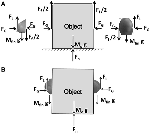
Figure 1. (A) A free body diagram showing the forces acting on object and finger. F_G, F_L, F_f, F_n stands for Grip, Lift, frictional, and normal forces, respectively. (B) The Figure showing the coupling between the finger and the object.

F_G is the grip force applied on the object horizontally acting in opposite directions. F_L is the lift force acting at the finger-object interface, lifting the object up. By the action of the F_G pressing on the object, and due to the friction between the finger and object, F_L gets coupled to the object. The forces thus emerging between the finger and object are shown in Figure 1B. The frictional force F_f acts on the object in the upward direction, with F_f/2 on either side of the object.

Figure 2A illustrates the interaction of F_L and F_G in controlling the position of the object (X_o). The model consists of two controllers (F_L and F_G controllers) and a plant. Inputs to the plant are F_L and F_G while the outputs are the object position (X_o), finger position (X_fin) and their derivatives (Ẋ_o, Ẍ_o, Ẋ_fin, Ẍ_fin). The objective of the control task is to lift the object to a reference position, X_ref. The model receives F_Gref and X_ref as the inputs and the X_fin (position of finger), X_o (position of object), Ẋ_fin (velocity of finger), Ẋ_o (velocity of object), Ẍ_fin (acceleration of finger) and Ẍ_o (acceleration of object) as outputs. The plant is described in detail in Appendix A.

FIGURE 2

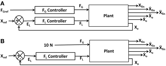
Figure 2. Block diagram showing (A) the interaction of the various components and their corresponding inputs and outputs. X, Ẋ, and Ẍ are the position, velocity, and acceleration; subscript “fin” and “o” denote finger and object, respectively; (B) the control loop used for F_L controller design. The grip force in the full system of panel (A) is set to a constant value of 10N.

The following sections describe the design of the controllers (F_G and F_L) followed by their training method, respectively.

The grip force (F_G) controller

The F_G controller (designed as a second order system) is used to generate the F_G which couples the fingers to the object. Typical F_G profiles of human subjects show a peak and a return to a steady state value, resembling the step-response of an underdamped second order system, thereby justifying the choice of an underdamped second order system as a minimal model. The F_G controller for a step input (F_Gref) is given in Equation (1).

$\begin{array}{cc}{F}_G=\frac{{\omega }_{\text{n}}{}^{\text{2}}}{({\text{s}}^{\text{2}}+2{\omega }_{\text{n}}\zeta \text{s}+{\omega }_{\text{n}}{}^{\text{2}})}& (1)\end{array}$

In order to determine the values of natural frequency, ω_n and damping factor, ζ, maximum overshoot (M_p, defined as the maximum peak value of the response curve) and time to peak (T_p, peaking time of the response curve) are required. Using prior published experimental values (Johansson and Westling, 1984) for M_p and T_p, F_G controller parameters are obtained using Equations (2, 3) (Ogata, 2002).

$\begin{array}{cc}{M}_p=e^{-\left(\zeta {\omega }_n/{\omega }_d\right)\pi }& (2)\end{array}$

$\begin{array}{cc}{T}_p=\frac{\pi }{{\omega }_{\text{d}}}& (3)\end{array}$

where ω_d the damped natural frequency is given as,

$\begin{array}{cc}{\omega }_d={\omega }_n\sqrt{1-{\zeta }^2}& (4)\end{array}$

See “Controller Training from the Model of The Precision Grip Control System” for the details of the above calculations.

Lift force (F_L) controller

The F_L controller, which is a Proportional-Integral-Derivative (PID) controller [Equation (5)], takes the position (E_L) as input [Equation (6)], and produces a time-varying F_L profile (F_L,PID) as output [Equation (5)] which in turn controls the object position.

$\begin{array}{cc}{F}_{L,\text{PID}}=K_{P,L}{E}_L+K_{I,L}{\displaystyle {\int }_0^T{E}_L}({\tau }_n)d{\tau }_n+K_{D,L}\frac{d{E}_L}{dT}& (5)\end{array}$

$\begin{array}{cc}{E}_L=X_{\text{o}}-X_{\text{ref}}& (6)\end{array}$

Here the K_P,L, K_I,L and K_D,L are the proportional, integral and derivative gains, respectively, for the F_L controller.

PID controller output is non-zero initially which is not realistic since the initial value of F_Lmust be zero. Hence, F_{L, PID} is smoothened using Equation (7).

$\begin{array}{cc}{\tau }_s\frac{d{F}_L}{dT}=-F_L+F_{L,\text{PID}}& (7)\end{array}$

where F_L (T = 0) = 0.

In order to design the F_L controller, we simplify the full system of Figure 2A as a F_L controller with a high constant F_G (10 N) to prevent the slip (Figure 2B). Note that if a constant and high value of F_G is assumed, slip is completely prevented, and the F_G controller is effectively eliminated from the complete system (Figure 2B). The F_L controller design now involves lifting a simple inertial load straight up from an initial position (X_o = 0 m) to a final position (X_o = 0.05 m).

Performance of the lift is evaluated using the cost function, CE, [Equation (8)]. This Cost function comprises of (1) average position difference between the finger (X_fin) and the object (X_o) at the end of the trial and (2) the difference in position between the desired and actual average position of the object.

$\begin{array}{cc}CE({\text{F}}_{\text{Gref}})=0.5{\left(\frac{{\overline{X}}_{\text{fin}}-{\overline{X}}_o}{{\overline{X}}_{\text{fin}}}\right)}^2+0.5{\left(\frac{X_{\text{ref}}-{\overline{X}}_o}{X_{\text{ref}}}\right)}^2& (8)\end{array}$

The F_L PID controller parameters were then optimized for cost function (CE) using Genetic Algorithm (GA) (Goldberg, 1989; Whitley, 1994) (refer Figure 3 for block diagram and for parameters refer Supplementary Material A) keeping F_G constant (=10 N) at a sufficiently high value so that the object does not slip.

FIGURE 3

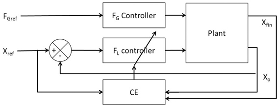
Figure 3. Block diagram showing the training mechanism of the F_L controller.

The F_L controller described above is designed assuming a constant and high grip force. But, when both F_G and F_L controllers are inserted in the full system (Figure 2A) the system may behave in a very different manner due to gradual F_G buildup starting from zero. When a step input of magnitude F_Gref is given to the F_G controller, the F_G starts from 0, then approaches a peak value and stabilizes at a steady-state value known as Stable Grip Force (SGF). Even with the trained controllers, for low values of F_Gref, the object may slip. But once the F_Gref is sufficiently high, slip is prevented and the object can be lifted successfully. Therefore, for a successful lift, an optimal value of F_Gref needs to be determined. The optimal F_Gref, which is related to SGF needed for a successful grip/lift performance, varies with the experimental setup, skin friction etc. (Ingvarsson et al., 1997; Fellows et al., 1998). It is here that we use concepts from RL and the utility function formulation for searching the F_Gref state space.

The Utility Function Formulation

The optimality of a decision is measured by the rewards fetched by it. Selection of an optimal choice providing the maximum expected value of the rewards (value) is known as optimal decision making (DM). DM can be seen in stock exchange, corporates and even our daily lives (which may or may not involve explicit monetary rewards). A lot of DM is carried out subconsciously when the person is unaware of the reason for choosing ones decision (Ferber et al., 1967). Non-human primates also show DM capabilities (Lakshminarayanan et al., 2011; Leathers and Olson, 2012). A mathematical framework is essential to empirically understand subjective DM behavior. Various independent studies confirm the role of value (average reward) and risk (variance in the rewards) in DM (Milton and Savage, 1948; Markowitz, 1952; Hanoch and Levy, 1969; Kahneman and Tversky, 1979; Bell, 1995; Lakshminarayanan et al., 2011).

A search for components of DM in the living world lead to identification neural correlates of value and risk in human and non-human primates (D'Acremont et al., 2009; Schultz, 2010; Lakshminarayanan et al., 2011; Leathers and Olson, 2012). Human DM process takes account of the risk in addition to the mean rewards that the decisions fetch. Furthermore, many neurobiological correlates of risk sensitivity are found in support of risk-based DM in humans (Wu et al., 2009; Schultz, 2010; Zhang et al., 2010; Wolpert and Landy, 2012).

An important instance of risk-based DM model is the utility function formulation, which is a combination of value and risk information (D'Acremont et al., 2009). The utility function used in the current model of PG performance derives from (Bell, 1995; D'Acremont et al., 2009) study that uses the concept of utility (U) as a weighted sum of value (V), which represents expected reward, and risk (h), which denotes variance in the reward. The weighting factor, λ, involved in the linear sum of V and h, denotes risk preference [Equation (9)].

$\begin{array}{cc}U=V-\lambda \sqrt{h}& (9)\end{array}$

We here introduce few terms from RL used in our study, following a policy (π) is associated with an expected value (V) of the state (s) at trial (t) is given by Equation (10).

$\begin{array}{cc}V(t)=E_{\pi }\left(r(t+1)+\gamma r(t+2)+{\gamma }^{2}r(t+3)+\dots |s(t)=s\right)& (10)\end{array}$

where, E is expectation and γ is the discount factor denoting the myopicity in the prediction of future rewards, and the reward is denoted by “r.” The V update is by Equation (11).

$\begin{array}{cc}V(t+1)=V(t)+{\eta }_V\delta (t)& (11)\end{array}$

where η_V is the learning rate for V and “δ” is the temporal difference error or the reward prediction error, and is given by Equation (12)

$\begin{array}{cc}\delta (t)=r(t+1)+\gamma V(t+1)-V(t)& (12)\end{array}$

Similarly, the risk prediction error, “ξ(t)” is denoted by Equation (13).

$\begin{array}{cc}\xi (t)=\delta {(t)}^2-h(t)& (13)\end{array}$

where, the risk function denoted by (h) is the variance in the prediction error [Equation (14)]

$\begin{array}{cc}h(t+1)=h(t)+{\eta }_{\text{risk}}\xi (t)& (14)\end{array}$

Here η_risk is the learning rate for risk. We now introduce a modified version of Utility (U) [Equation (9)], as follows,

$\begin{array}{cc}U(t)=V(t)-\alpha \text{sign}(V(t))\sqrt{h(t)}& (15)\end{array}$

where “α sign(V(t))” is the risk preference (Pragathi Priyadharsini et al., 2012).

The sign(V) term achieves a familiar feature of human decision making viz., risk-aversion for gains and risk-seeking for losses (Kahneman and Tversky, 1979). In other words, when V is positive (negative), U is maximized (minimized) by minimizing (maximizing) risk. We now use the above basic framework for modeling the Utility as a function of F_Gref.

Computing U(F_Gref)

We now explain how the above-described Utility function formulation is applied in the present study. The Utility function, U, and its components V and h, are expressed as functions of F_Gref, which is taken as the state variable. A given value of F_Gref results in either slip or successful lift of an object. The measure of performance is expressed by CE [Equation (8)].

The value “V” and risk “h” are computed as a function of F_Gref by repeatedly simulating lift for a range of values around F_Gref. This helps us to analyze the possible variability caused on the performance of the PG task with F_Gref. A range of values were obtained by adding uniformly distributed noise (ν : refer Table 1) to F_Gref [Equation (16)]. We modeled ν to proportionally represent the F_slip i.e., the value of ν is increased for a low μ.

$\begin{array}{cc}{\widehat{F}}_{\text{Gref}}=F_{\text{Gref}}+\nu & (16)\end{array}$

TABLE 1

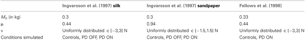
Table 1. Parameters used in simulation: Mass of the object (M_o), friction coefficient (μ) and noise added (ν) for different cases simulated in the study.

For the given value of F_Gref, V_CE was drawn from the performance measure [Equation (8)] and is generated using the cost function CE as [Equation (17)]. Refer Figure 4 for the block diagram for determining V_CE.

$\begin{array}{cc}{V}_{CE}\left({\widehat{F}}_{\text{Gref}}\right)=e^{-CE\left({\widehat{F}}_{\text{Gref}}\right)}& (17)\end{array}$

FIGURE 4

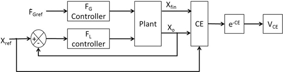
Figure 4. Block diagram showing the generation of error function (V_CE) for the input F_Gref.

There is no explicit reward in the present formulation. V_CE represents a reward-like quantity, the average of which is linked to value. Value [Equation (18)] and risk [Equation (19)] were calculated as the mean and variance of the V_CE,

$\begin{array}{cc}V\left(F_{\text{Gref}}\right)=\text{mean}\left(V_{CE}\left({\widehat{F}}_{\text{Gref}}\right)\right)& (18\end{array})$

$\begin{array}{cc}h\left(F_{\text{Gref}}\right)=\text{var}\left(V_{CE}\left({\widehat{F}}_{\text{Gref}}\right)\right)& (19)\end{array}$

We now have a set of numerical values of F_Gref and the corresponding V and h values. These numerical values are used to construct V and h as explicit functions of F_Gref using Radial Basis Function Neural Networks (RBFNNs) explained in Appendix B. The above mentioned Equations (18, 19) is general to all the trials. These processes are summarized in Table 2.

TABLE 2

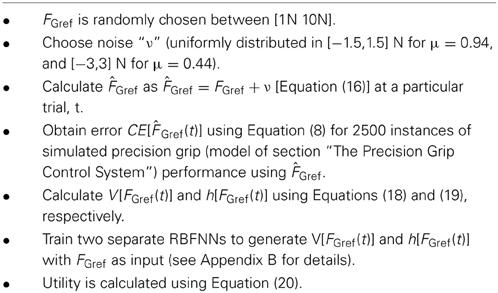
Table 2. Steps to train value = V(F_Gref) and risk = h(F_Gref).

Specifically, for a F_Gref chosen at trial, t, U(F_Gref(t)) is a combination of the V(F_Gref(t)) and h(F_Gref(t)). Utility, U(F_Gref(t)) [Equation (20)], is then obtained in terms of V and h, as shown below:

$\begin{array}{cc}U\left(F_{\text{Gref}}(\text{t})\right)=V\left(F_{\text{Gref}}(\text{t})\right)-\alpha \sqrt{h\left(F_{\text{Gref}}(\text{t})\right)}& (20)\end{array}$

Decisions are made by choosing actions that maximize U(F_Gref(t)). Increasing the value of α makes the decision more risk aversive, while the decisions are more risk-seeking for smaller values of α. Maximizing U(F_Gref(t)) is done by a stochastic hill-climbing process called the “Go/Explore/NoGo” (GEN) method. This method is inspired by dynamics of the BG and was described in greater detail in earlier work (Magdoom et al., 2011). We now present a brief account of the GEN method.

Modeling Precision Grip Performance as Risk-Based Action Selection

The key underlying idea of the proposed model is to treat the problem of choosing the right F_G as an action selection problem and thereby suggest a link between the action selection function of the BG and PG performance. Impairment in action selection machinery of the BG under PD conditions is then invoked to explain F_G changes in PD ON and OFF conditions.

In line with the tradition of Actor-Critic approach to modeling the BG (Joel et al., 2002); we recently proposed a model of the BG in which value is thought to be computed in the striatum. Furthermore, we hypothesized that the action selection function of the Basal Ganglia is accomplished by performing some sort of a stochastic hill-climbing over the value function computed in the striatum. We dubbed this stochastic hill-climbing method the “Go/Explore/NoGo” (GEN) method (Magdoom et al., 2011; Kalva et al., 2012), which denotes a conceptual expansion of the classical Go/NoGo picture of the BG function. As an extension of the above model, we had recently proposed a model of the BG in which the striatum computes not just value but the Utility function (Pragathi Priyadharsini et al., 2012). Action selection is then achieved by applying the GEN method to the Utility function. In the present study, we apply the GEN method to the Utility function and estimate grip forces in control and PD conditions.

Neurobiological interpretation of the GEN method in controls

We now present some background and neurobiological interpretation of the GEN method in connection with functional understanding of the BG, following which details of the GEN method will be provided.

The BG system consists of 7 nuclei situated on two parallel pathways that form loops—known as the direct pathway (DP) and the indirect pathway (IP)—starting from the cortex and returning to the cortex via the thalamus. Striatum is the input port of the BG, which receives inputs from the cortex. The Globus Pallidus interna (GPi) and the Substantia Nigra pars reticulata (SNr) are the output ports that project to thalamic nuclei, which in turn project to the cortex, closing the loop. The DP consists of the striatum projecting directly to GPi/SNr, while the IP consists of a longer route starting from the striatum and returning to GPi/SNr via Globus Pallidus externa (GPe) and the Subthalamic Nucleus (STN) in that order. The striatum receives dopaminergic projections from the Substantia Nigra pars compacta (SNc) (Mink, 1996; Smith et al., 1998). Striatal dopamine levels are thought to switch between DP and IP, since the DP (IP) is selected for higher (lower) levels of dopamine (Sutton and Barto, 1998; Frank, 2005; Wu et al., 2009) (Figure 5).

FIGURE 5

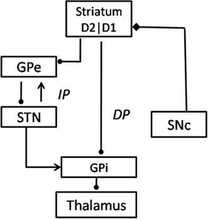
Figure 5. The Basal Ganglia network with DP (Direct Pathway) and IP (Indirect Pathway) specified.

In classical accounts of the BG function, the DP is known as the Go pathway since it facilitates movement and the IP is called the NoGo pathway since it inhibits movement. Striatal dopamine levels are thought to switch between Go and NoGo regimes (Albin et al., 1989). We have been developing a view of the BG modeling in which the classical Go/NoGo picture is expanded to Go/Explore/NoGo picture, wherein a new Explore regime is inserted between the classical Go and NoGo regimes (Kalva et al., 2012). This explore regime corresponds to random exploration of action space which is a necessary ingredient of any RL machinery. Kalva et al. (2012) show that the Explore regime arises naturally due to the chaotic dynamics of the STN-GPe loop in the IP. The three regimes together amount to a stochastic hill-climbing, which we describe as the GEN method. The GEN method has been used in the past to describe a variety of functions of the BG, in control and PD conditions, including reaching movements (Magdoom et al., 2011) and spatial navigation (Sukumar et al., 2012).

Magdoom et al. (2011) used the GEN method to hill-climb over the value function (Magdoom et al., 2011). δ_V(t) is defined as a temporal difference in value function [Equation (21)].

$\begin{array}{cc}{\delta }_V(t)=V(F_{\text{Gref}}(t))-V(F_{\text{Gref}}(t-1))& (21)\end{array}$

where “t” is not “time” but “trial number.”

The GEN method used in Magdoom et al. (2011) can be summarized using the following Equation (22),

$\begin{array}{cc}\begin{array}{l}\text{if}({\delta }_V(t)>D{A}_{hi})\hfill \\ \begin{array}{ccc}\mathrm{ \Delta }{F}_{\text{Gref}}(t)=+\Delta F_{\text{Gref}}(t-1)\hfill & -“{\text{Go}}^{\prime \prime }\hfill & (\text{a})\hfill \end{array}\hfill \\ \text{else if}({\delta }_V(t)>D{A}_{lo}\wedge {\delta }_V(t)\le D{A}_{hi})\hfill \\ \begin{array}{ccc}\mathrm{ \Delta }{F}_{\text{Gref}}(t)=\psi \hfill & -“\text{E}xp{\text{lore}}^{\prime \prime }\hfill & (\text{b})\hfill \end{array}\hfill \\ \text{else}({\delta }_V(t)\le D{A}_{lo})\hfill \\ \begin{array}{ccc}\mathrm{ \Delta }{F}_{\text{Gref}}(t)=-\Delta F_{\text{Gref}}(t-1)\hfill & -“{\text{NoGo}}^{\prime \prime }\hfill & (\text{c})\hfill \end{array}\hfill \end{array}& (22)\hfill \end{array}$

where, ψ is a random vector, and ||ψ|| = χ, a positive constant. DA_hi and DA_lo are the thresholds at which dynamics switches between Go, NoGo and Explore regimes [Equation (22)]. The underlying logic of the above set of Equations (22a–c) is as follows. If δ_V(t) > DA_hi, the last update resulted in a sufficiently large increase in V; therefore continue in the same direction in the next step. This case is called the “Go” (Equation 22a) regime. If δ_V(t) ≤ DA_lo, the last update resulted in a significant decrease in V; therefore proceed in the direction opposite to the previous step. This case is called the “NoGo” (Equation 22b) regime. If DA_lo < δ_V(t) ≤ DA_hi, there was neither a marked increase nor decrease in V; therefore Explore (Equation 22c) for new directions. This case is called the Explore regime. In Magdoom et al. (2011) we assumed a simple symmetry between DA_hi and DA_lo, such that DA_hi > 0 and DA_lo = −DA_hi.

However, in the present study we introduce a small variation of the above formulation of the GEN method. Instead of V, we perform hill-climbing over the Utility landscape. The three separate Equations (22a–c) can be combined into a single Equation (23) [as in Sukumar et al. (2012)], as follows:

$\begin{array}{cc}\begin{array}{l}\Delta F_{\text{Gref}}(t)=A_G\log \text{sig}\left({\lambda }_G{\delta }_U(t)\right)\Delta F_{\text{Gref}}(t-1)\hfill \\ -A_N\log \text{sig}({\lambda }_N{\delta }_U(t))\Delta F_{\text{Gref}}(t-1)\hfill \\ +A_E\psi \exp (-{\delta }_U^2(t)/{\sigma }_E^2)\hfill \end{array}& (23)\end{array}$

where,

$\begin{array}{cc}{\delta }_U(t)=U\left(F_{\text{Gref}}(t)\right)-U\left(F_{\text{Gref}}(t-1)\right)& (24)\end{array}$

And,

$\begin{array}{cc}\text{logsig}(n)=\frac{1}{1+\text{exp}(-n)}& (25)\end{array}$

ΔF_Gref is the change in F_Gref and ‘t’ is the trial number; A_G/E/N are the gains of Go/Explore/NoGo components, respectively; λ_G/N are the sensitivities of the Go/NoGo components, respectively; ψ is a random variable uniformly distributed between −1 and 1 and σ_E is the standard deviation used for the Explore component.

Just as TD error is interpreted as dopamine signal in classical RL-based accounts of the BG function, we interpret δ_U as dopamine signal in the present study. In Equation (23) above, the first term on the RHS corresponds to “Go” regime, since it is significant for large positive values of δ_U (since A_G and λ_G are positive). The second term on the RHS of Equation (23) above corresponds to “NoGo” regime, since it is significant for large negative values of δ_U (due to A_N > 0 and λ_G < 0). The third term on the RHS corresponds to “Explore” regime, since it is dominant for values of δ_U close to 0.

Neurobiological interpretation of the GEN method in PD

PD being a dopamine deficient condition, a natural way to incorporate Parkinsonian pathology is to attenuate the dopamine signal, δ_U. In (Magdoom et al., 2011; Sukumar et al., 2012), PD pathology was modeled by clamping the dopamine signal, δ_U, and preventing it from exceeding an upper threshold. The rationale behind such clamping is that with fewer dopaminergic neurons left, SNc may not be able to produce a signal intensity that exceeds a certain threshold. In the present case of PG, such a constraint is applied to δ_U. If [a,b] is the natural unconstrained range of values of δ_U for controls, then for PD OFF simulation, a clamped value of δ_Lim changes the δ_U range to [a, δ_Lim] where δ_Lim < b. Furthermore, to simulate the increase in dopamine levels in PD ON condition, due to administration of L-dopa, a positive constant is added to δ_U, thereby changing the range of δ_U in PD ON condition to [a+ δ_Med, δ_Lim + δ_Med] [Equation (26)].

$\begin{array}{cc}{\delta }_{\text{U}}(t)=\{\begin{array}{l}[a,b](\text{a})\text{for}\text{controls}\hfill \\ [a,{\delta }_{\text{Lim}}](\text{b})\text{for}\text{PD}\text{OFF}\hfill \\ [a+{\delta }_{\text{Med}},{\delta }_{\text{Lim}}+{\delta }_{\text{Med}}](\text{c})\text{for}\text{PD}\text{ON}\hfill \end{array}& (26)\end{array}$

where δ_Lim + δ_Med < b and a < b.

Training the GEN parameters

The output of the GEN system is F_G from which SGF is calculated as average F_G between 4000 and 5000 ms of simulation time, the mean and variance of which must match with the mean and variance of SGF obtained from PG experiments under control and PD conditions (Ingvarsson et al., 1997; Fellows et al., 1998). The parameters to be trained are A_G/E/N [gains of the Go/Explore/NoGo terms in Equation (23)], λ_G/N [sensitivity of Go/NoGo terms in Equation (23)] and σ_E [sensitivity of Explore term in Equation (23)]. Determination of the GEN parameters is done by optimizing a cost function CE_GEN given as.

$\begin{array}{cc}C{E}_{\text{GEN}}=2{\left({\overline{SGF}}_{expt}-{\overline{SGF}}_{\text{sim}}\right)}^2+{\left({\sigma }_{expt}-{\sigma }_{\text{sim}}\right)}^2& (27)\end{array}$

SGF is the stable grip force generated and σ is the variance in the error. Subscripts expt and sim denote experimental and simulated values, respectively. CE_GEN is formulated such that more weightage is given to the SGF error and lesser to the variance in the error [Equation (27)].

The six model parameters (A_G/E/N, λ_G/N, and σ_E) of the GEN method [Equation (23)] are trained to capture the following experimental conditions: Controls and PD ON conditions are obtained from Fellows et al. (1998), whereas controls, PD ON and OFF from Ingvarsson et al. (1997) for both sandpaper and silk surfaces. However, the parameters A_G/E/N, λ_G/N, and σ_E are not all trained separately for every experimental condition. Initial parameter values for A_G/E/N, λ_G/N, σ_E, and α were determined (Figure 6A) by matching the SGF results for controls of Fellows et al. (1998); this matching is achieved by optimizing CE_GEN [Equation (27)] using GA (Figure 6A). This initial training of GEN parameters is a kind of calibration of the parameters for a given experimental setup. Once an initial estimate of parameters was obtained, A_G/E/N, λ_G/N, and σ_E were fixed and optimal values of α, δ_Lim, and δ_Med were obtained using GA for the PD conditions, of Fellows et al. (1998). Similarly, for Ingvarsson et al. (1997), the initial parameter values for A_G/E/N, λ_G/N, σ_E, and α were determined by matching the SGF results for controls using Equation (27). For the cases of PD ON and PD OFF (Ingvarsson et al., 1997), the search space was limited to α, δ_Lim, δ_Med, by having fixed the values of A_G/E/N, λ_G/N, σ_E obtained from controls (Ingvarsson et al., 1997).

FIGURE 6

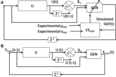
Figure 6. Block diagram showing (A) training of GEN parameters using CE_GEN; (B) model testing using trained GEN parameters.

The model was tested (Figure 6B) using the trained GEN parameters to determine if the model generated outputs are close to the experimental values.

Results

We now apply the model described in the previous section to explain the experimental results for two published studies (Ingvarsson et al., 1997; Fellows et al., 1998). For simplicity we used only constant weight trials (i.e., only the trials where only one load was repeatedly used for lifting). The friction coefficient was calculated as load force/slip force (Forssberg et al., 1995) [Equation (28)].

$\begin{array}{cc}\mu =M_{o}g/F_{\text{slip}}& (28)\end{array}$

Fellows et al. (1998) investigated 12 controls, 16 PD patients and four hemi-parkinsonian patients. All the PD subjects were in medication ON state. The subjects were asked to lift the object to a height of 4–8 cm. The study comprised of two loads 3.3 N and 7.3 N. Various combinations of these two loads were used to give rise to “light,” “heavy,” “unload,” and “load” condition. In our study, we simulated only the experimental results for the “light” condition (which featured lifting the 3.3 N object for all the trials) with a desired object lift height of 5 cm.

Ingvarsson et al. (1997) investigated the role of medication in 10 controls and 10 PD subjects under two object surface conditions (silk and sandpaper). The task required the object to be PG–lifted to a height of 5 cm above the table. The entire experiment was divided into 3 parts (a) coordination of forces, (b) adaptation to friction and (c) rapid load changes. “Coordination of forces” required the object to be lifted to 5 cm height, and maintained at that position for 4–6 s using PG. “Adaptation to friction” required the subjects to gradually reduce the grip force on the object thereby causing slip F_slip is calculated. Finally, in the “rapid load changes” task a plastic disk was dropped in a padded plate thereby causing abrupt changes in F_L.

In the present study, we use the F_slip for determining the friction coefficient which is used to match the experimentally obtained grip force values under silk and sandpaper condition for coordination of forces case. Ingvarsson et al. (1997) reported the results in median ± Q3 quartile format. Hence for simplicity the results are assumed to be normally distributed with mean = median and Q3 = mean + 0.6745 standard deviation. The entire text reports the results in terms of mean and variance.

We now describe the simulation results starting from controller training to simulation of results from Ingvarsson et al. (1997) and Fellows et al. (1998).

Controller Training From the Model of the Precision Grip Control System

The F_G controller

In the present model the grip force controller is designed as reference tracking controller which receives F_Gref as the input and generates a time-varying F_G(T) as the output. So in the proposed configuration the F_G controller is only affected by the input (F_Gref) it receives. Using the overshoot ratio, M_p = 1.25, [Equation (2)] and time to peak, T_p = 530 ms, [Equation (3)] as design criteria [M_p and T_p values obtained from Johansson and Westling (1984)], we determined ω_n = 6.4 and ζ = 0.4 as the parameters for transfer function of the F_G controller [Equation (1) in The Precision Grip Control System; Ogata, 2002]. Figure 7A shows the grip force profile (for T = 5000 ms) for the input F_Gref = 10 N. Since the F_G controller is modeled as a transfer function which is dependent only on the F_Gref value, the controller did not require retraining for different friction conditions.

FIGURE 7

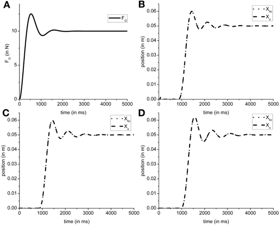
Figure 7. Figure shows a single trial simulated output obtained from model. (A) The typical F_G profile for the input F_Gref = 10 N. The object and finger position for (B) Ingvarsson et al. (1997) silk (μ = 0.44, M_o = 0.3 kg); (C) Ingvarsson et al. (1997) sandpaper (μ = 0.94, M_o = 0.3 kg); (D) Fellows et al. (1998) (μ = 0.44, M_o = 0.33 kg) are shown. Note that in generation of (B–D), the F_Gref is kept constant at 10 N for illustration purpose.

The F_L controller

The efficacy of F_L controller output can be observed in the output object and finger position. If a suboptimal F_L is generated, the object does not reach the reference position. The cardinal components affecting the object-finger slip are μ and M_o (Refer Table 1 for the values of μ and M_o used in simulation). Since the F_L controller is affected by μ and M_o, a decreased μ or increased M_o increases the F_slip Therefore, in this study we trained the F_L controller for the minimum μ and the maximum M_o to prevent the object from slipping even when μ increases or M_o decreases. Furthermore, to train the F_G controller, we assume a sufficiently large F_G (=10 N) thereby effectively decoupling the F_G controller. With a large, constant F_G, the cost function (CE) [Equation (8)] was optimized using the GA (Goldberg, 1989; Whitley, 1994) for the setup parameters from Fellows et al. (1998) (μ = 0.44 and M_o = 0.33 N) to obtain PID parameter values. The PID parameter values obtained were K_P,L = 6.938, K_I,L = 14.484, K_D,L = 1.387, τ_s = 0.087. The same PID parameters were used to simulate results from Ingvarsson et al. (1997) also. In Figure 7, the output of the simulated finger and object position is shown for (Figure 7B) the silk condition of (Ingvarsson et al., 1997), (Figure 7C) the sandpaper condition of (Ingvarsson et al., 1997) and (Figure 7D) light condition of (Fellows et al., 1998).

Since we fixed the PID parameters for the F_L controller, efficacy of the PID parameters across the three control conditions viz. Ingvarsson et al. (1997) silk condition, Ingvarsson et al. (1997) sandpaper, and Fellows et al. (1998), needs to be determined. Two important criteria for determining a successful lift are: low slip (X_fin − X_o) and low position error (X_ref − X_o). In all the three cases (refer Table 1) the finger–object slip distance was <0.005 m and the X_ref − X_o <0.001 m, where, X_o is average position between simulation time (T) as 4000 and 5000 ms. The F_G controller output is shown in Figure 7A; object and hand position for Ingvarsson et al. (1997) sandpaper, Ingvarsson et al. (1997) sandpaper, and Fellows et al. (1998) is shown in Figures 7B–D. Note that F_Gref is held constant at 10 N.

Obtaining V(F_Gref), H(F_Gref), and U(F_Gref)

Utility based approach requires estimation of V(F_Gref) and h(F_Gref) [refer model Section “Computing U(F_Gref)”]. V and h are generated for Ingvarsson silk and Ingvarsson sandpaper and were obtained using the parameters given in Table 1. We assumed the noise to be inversely related to the friction coefficient. Hence a higher noise was used in case of lower μ and vice versa.

Note that value functions [expressed as a function of F_Gref (Appendix B, Equation (42)] in case of PG are expected to have a sigmoidal shape, since a F_G level that exceeds the F_slip always results in a successful grip-lift and therefore reward. On the contrary, the risk function, h [Appendix B, Equation (43)], is expected to be bell-shaped since risk is the highest in the neighborhood of slip force, and zero far from it.

These observations are supported by the value and risk functions constructed for various experimental conditions —Fellows et al. (1998) light and Ingvarsson et al. (1997) silk and sandpaper cases. Figure 8A shows the value and risk functions for Fellows et al. (1998), Figure 8B shows the value and risk functions for Ingvarsson et al. (1997) silk and Figure 8C shows the value and risk functions for Ingvarsson et al. (1997) sandpaper condition.

FIGURE 8

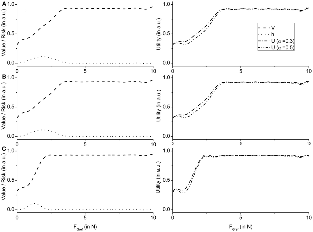
Figure 8. Figure showing the value, risk and utility (α = 0.3 and α = 0.5) of the RBF network as an average value of 20 runs for (A) Fellows et al. (1998) (B) Ingvarsson et al. (1997) silk, and (C) Ingvarsson et al. (1997) sandpaper.

Performing Action Selection Using the BG and Simulating the Control and PD Cases of the Study

Two features mark the difference in V(F_Gref) and h(F_Gref) between controls and PD. In PD OFF case we apply the clamped δ_U(=δ_Lim) condition [Equation (26b)], whereas in PD ON case we add a positive constant (δ_Med) to δ_U [Equation (26c)]. In addition to these changes in the dopamine signal, δ_U, we assume altered risk sensitivity in PD. Studies also suggest altered risk taking in PD patients (in particular, risk in PD ON> risk in PD OFF) when compared to healthy controls (Cools et al., 2003). Since α represents risk sensitivity in the utility function [Equation (20)], we use a smaller α in PD case (both ON and OFF) (Refer Tables 3, 4 for the simulated values).

TABLE 3

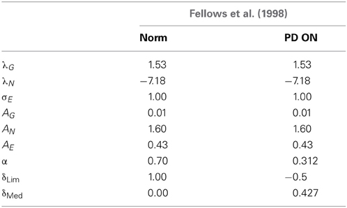
Table 3. Table showing the GEN parameters and Utility parameters for Fellows et al. (1998) control and PD ON.

TABLE 4

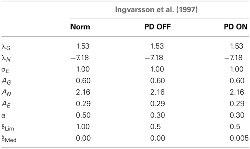
Table 4. Table showing the GEN parameters and Utility parameters for simulating both Ingvarsson et al. (1997) cases of silk and sandpaper in controls, PD OFF and PD ON conditions.

As described earlier, the GEN method [Equation (23)], produces a series of SGF values with a certain mean and standard deviation computed over the trials. It may be recalled, from “Model”, that Equation (23) represents a form of stochastic hill-climbing over the utility function, U. It represents a map from F_Gref (t − 1) to F_Gref (t), where “t” represents the trial number. The three terms on the RHS of Equation (23) represent GO, NOGO and Explore regimes, in that order. The three regimes are active under conditions of high, low, and moderate dopamine (δ_U), respectively. Figure 9 shows some sample profiles of the three terms on the RHS of Equation (23).

FIGURE 9

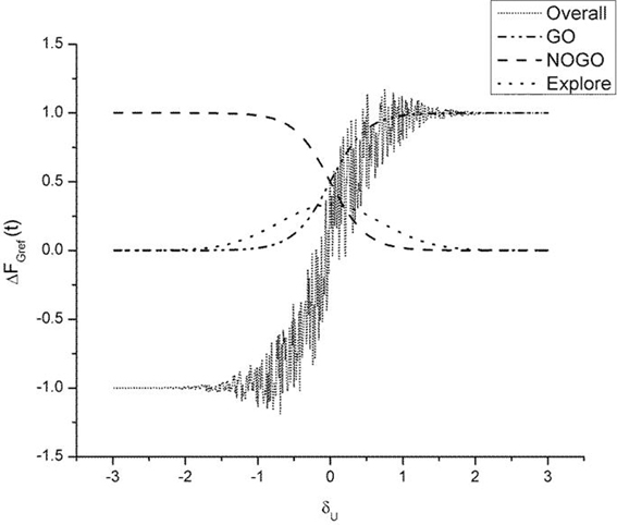
Figure 9. Figure illustrating output of the GO (λ_G = 2), NOGO (λ_N = −2), explore (σ_E = 1) regime and the overall output of the three regimes. Here A_G = A_N = A_E = 1. The ΔF_Gref(t − 1) is set to 1. We thereby analyze the selection output ΔF_Gref(t) as a function of δ_U alone. The “overall” graph is produced by actually adding the noise term [III term on RHS in Equation (23)]. Note the high variability in ΔF_Gref(t) in the vicinity of δ_U = 0.

Using the GEN policy on δ_U, we simulate our model with parameters described in Tables 3, 4 (However, simulation with δ_V of Equation (21) with the same parameter set described in this section yields Supplementary Material B).

Procedure to train the GEN parameters

• The change in F_Gref (i.e., ΔF_Gref) from trial, “t” to “t+1” is given in Equation (23).

• This Equation (23) contains six parameters (A_G/E/N, λ_G/N and σ_E) whose values need to be determined.

• The training for GEN parameters (A_G/E/N, λ_G/N and σ_E) was carried out using GA for optimizing CE_GEN on Fellows et al. (1998) control condition experimental data. (Figure 6A)

• The GEN parameters obtained from the control conditions are also used for simulating PD. In case of (Fellows et al., 1998), the parameters from controls are used for PD ON only. In case of (Ingvarsson et al., 1997), the parameters from controls are used in PD ON and OFF for two surface conditions – silk and sandpaper.

• In PD OFF case, only δ_Lim and α are trained. In PD ON case, δ_Lim, δ_Med and α are trained.

Simulation of Fellows et al. (1998) results

Fellows et al. (1998) for controls was simulated using the parameters (Table 4) obtained by optimizing GA on CE_GEN.

(a) Using the A_G/E/N, λ_G/N, σ_E and α = 0.7 obtained from the GA, the controls was simulated using δ_Lim = 1 and δ_Med = 0.

(b) A similar approach was performed for modeling the PD ON condition. The parameters (A_G/E/N, λ_G/N and σ_E) were the same as the controls, while the values of α = 0.312, δ_Lim = −0.5 and δ_Med = 0.427 were obtained by GA optimization. For a detailed list of parameters see Table 3.

A comparison of the experimental and simulated data obtained for Fellows et al. (1998) using the parameters in Table 3 is given as Figure 10.

FIGURE 10

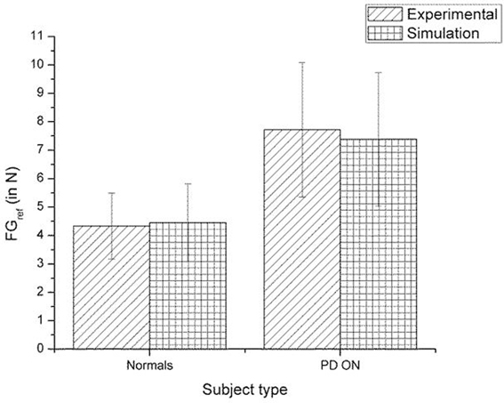
Figure 10. Comparison of experimental (Fellows et al., 1998) and simulation results for SGF. The bars represent mean (±SEM). The results for the control and PD ON groups are statistically significant with the p-value < 0.05 in both the experiment and simulation.

Simulation of Ingvarsson et al. (1997) results

Following the simulation of the Fellows et al. experiment:

(a) The results of the Ingvarsson et al. (1997) controls for both sandpaper and silk were simulated for obtaining (A_G/E/N, λ_G/N, σ_E, and α = 0.5) using GA (Table 4). The other parameters are set as δ_Lim = 1 and δ_Med = 0.

(b) In PD ON condition, the same control parameters (A_G/E/N, λ_G/Nand σ_E) were used along with α = 0.30, δ_Lim = 0.5 and δ_Med = 0.005 obtained through GA optimization.

(c) PD OFF condition was shown by optimizing α = 0.30, δ_Lim = 0.5 and δ_Med = 0 with the parameters (A_G/E/N, λ_G/Nand σ_E) remaining the same as that of the controls.

A comparison of the experimental and simulated data obtained for Ingvarsson et al. (1997) for silk and sandpaper using the parameters in Table 4 is given as Figures 11 and 12, respectively. In order to be consistent with the experimental result the simulation results in Figures 11 and 12 are shown in median ± Q3. Figures 10–12 replicate the empirical findings (both mean / median and variance profiles) well. Fellows et al. (1998) results show that the mean(SGF) is higher in PD ON case compared to controls (SGFnorm<SGF_PDON) (Figure 10). A similar result (SGFnorm<SGF_PDON) is also reported in Ingvarsson et al. (1997) silk (Figure 11) and sandpaper cases (Figure 12). Furthermore, var(SGF) under PD OFF cases is observed to be greater than that of controls. It may be inferred that the increase in SGF during the PD conditions would be due to their increased SM while playing risk aversive in the game of risk based decision making. This increased SM could be needed to oppose the increased internal perturbations/sensory-motor incoordination observed in the PD patients.

FIGURE 11

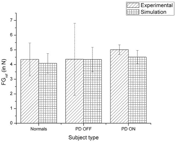
Figure 11. Comparison of experimental (Ingvarsson et al., 1997) and simulation results for SGF for silk surface. The bars represent the median (± Q3 quartile). The results for the control and PD ON groups are statistically significant with the p-value < 0.05.

FIGURE 12

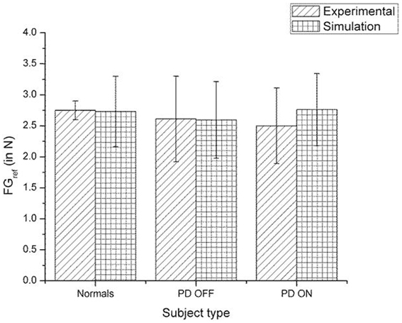
Figure 12. Comparison of experimental (Ingvarsson et al., 1997) and simulation results for SGF for sandpaper surface. The bars represent the median (± Q3 quartile). The results for the comparison on controls-PD ON, controls-PD OFF and PD ON-PD OFF in both the experiment and simulation are non-significant in both the experiment and simulation.

Discussion

In this paper, we present a computational model to explain the changes in F_G in controls and PD ON/OFF conditions (Ingvarsson et al., 1997; Fellows et al., 1998). To our knowledge this is the first computational model of PG performance in PD conditions. A novel aspect of the proposed approach to modeling PG is to apply (based on the observation that PG performance involves a SM) concepts from risk-based DM to explain F_G generation. To this end, we applied a recent model of the BG action selection based on the utility function formulation, instead of value function, to explain PG performance (Pragathi Priyadharsini et al., 2012).

There are significant challenges involved in developing a computational model of PG in PD conditions. The root cause of this difficulty is that the pathology in PD is located at a high level (dopaminergic neurons of the BG) in motor hierarchy, while the motor expression is at the lowest level in the hierarchy (finger forces). Ideally speaking, a faithful computational model must incorporate these two well-separated levels in motor hierarchy, and all the levels in between. But development of such an extensive model would be practically infeasible, and may not be essential to the problem at hand. On the other hand, if model compactness is the sole governing principle, one may build an empirical, data-fitting model that links experimental parameters like friction, object weight, and abstract neural parameters like dopamine level, medication level, with observed data like mean and variance of grip force generated. But such an over-simplified model could be a futile mathematical exercise without much neurobiological content.

Therefore, a conservative approach to model PG performance in PD would have two components: (1) a minimal model of sensory-motor loop dynamics involved in generating PG forces, and (2) a minimal model of the BG that incorporates the effect of dopamine changes on the BG dynamics. Whereas the BG level generates evaluations of actions (F_G) based on the rewards (successful grip performance) obtained from PG performance, the sensory-motor loop dynamics receives the command from the BG level and generates F_G. While the first component represents DM, the second represents execution. These two components must then be integrated. PD-related reduction in dopamine level in the integrated model must then be manifested as appropriate changes seen in PG forces. This is the approach adopted in the present study. Figure 13 presents the grand plan of the entire model, and the training/design steps followed to build various components.

FIGURE 13

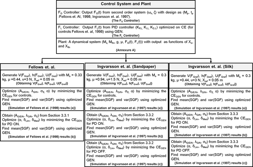
Figure 13. An illustration of the entire model, the training/design steps followed to build various components and to reproduce the results of Fellows et al. (1998) and Ingvarsson et al. (1997). The text in {} denote section name.

Modeling the Sensorimotor Loop

The sensory-motor loop component consists of two controllers, for generating the grip force and lift force, and a plant model. F_G and F_L and given as inputs to the plant model which simulates the of the object and the fingers. The error between actual and desired object positions is fed back to the F_L controller. The F_G controller receives F_Gref as input and generates the F_G(T) profile. F_Gref is generated by the second component, the BG component, by a DM process. The BG component is built on the lines of Actor-Critic models of the BG, where the utility function used instead of value function, and the dopamine signal, δ, is the temporal difference of utility [Equation (24)].

The F_LController Forms a Loop with the Plant

The controller gives F_L as input to the plant and receives position error as feedback. The controller is trained by GA as described in “The Precision Grip Control System”. The grip force controller is designed as an open-loop second order system that gives F_G as input to the plant (see The “Precision Grip Control System”). Plant dynamics is described in Appendix A. The controller and plant system, with its trained parameters, is then integrated with appropriately trained the BG models to simulate control and PD results (Ingvarsson et al., 1997; Fellows et al., 1998).

Simulation of Fellows et al. (1998) results

Incorporating the values of object mass (M_o = 0.33 kg) and friction (μ = 0.44) from Fellows et al. (1998), the controller and plant system trained above is used to calculate V and h functions (see “The Precision Grip Control System”). The V and h functions thus computed are explicitly modeled using RBFNNs (see “The Utility Function Formulation”). The V and h functions are combined to produce the utility function, which is used in the GEN method [see “Computing U(F_Gref)”] to produce mean(SGF) and var(SGF) as outputs. The parameters of the GEN method must be calibrated to each experimental setup. Thus, the GEN parameters (A_G/E/N, λ_G/Nand σ_E) are trained by GA to produce the mean(SGF) and var(SGF) corresponding to the controls case. Then for the PD ON case, only δ_Lim and δ_Med are optimized (A_G/E/N, λ_G/N and σ_E are unchanged). Simulated and experimental values of mean(SGF) and var(SGF) approximate the experimental mean(SGF) and var(SGF) (see Results: Figures 11, 12).

Simulation of Ingvarsson et al. (1997) results

The case of Ingvarsson et al. (1997) is a bit more complicated since it involves two friction conditions: silk and sandpaper. It also involves both PD ON and OFF unlike Fellows et al. (1998) which describes results for only PD ON. For the condition of sandpaper, object mass (M_o = 0.3 kg) and friction (μ = 0.94) are incorporated into the trained controller and plant system. V and h functions are computed and explicitly modeled using RBFNNs (“The Utility Function Formulation”) and Utility function is computed by combining V and h. The Utility function is used in the GEN method; the GEN parameters (A_G/E/N, λ_G/N and σ_E) are trained to minimize CE_GEN[Equation (27), Figure 5] so as to calibrate the model for the sandpaper case of Ingvarsson et al. (1997). The trained GEN parameters are used for the PD OFF case and only δ_Lim is trained to optimize CE_GEN. The same GEN parameters are again used for the PD ON case, where both δ_Lim and δ_Med are optimized. A similar procedure is followed for the “silk” case (M_o = 0.3 kg and μ = 0.44) of Ingvarsson et al. (1997) as outlined in Figure 13.

Risk-based decision making can arise in both motor and cognitive domains (Claassen et al., 2011). The present study deals with risk in motor domain. In this context, an interesting question naturally arises. Is there a correlation between risk-sensitivity in motor and cognitive domains. Does impaired risk-sensitivity in one domain carry over to the other? In other words, do PD patients show impaired decision making in motor and cognitive domains equally? In order to answer the above line of questioning, we propose to use a task, the Balloon Analog Risk Task (BART), which tests risk-sensitivity in cognitive domain (Claassen et al., 2011). We then propose to adapt that BART to the motor domain.

In BART, the subject is asked to press a key and inflate a virtual balloon displayed on the monitor. For every key press, the virtual balloon is inflated by a fixed amount and the subject earns a fixed number of points. The catch lies in that, on inflation beyond a threshold volume, the balloon bursts and the subject loses all the points. Knowing when to stop and redeem all the points earned so far involves risk based decision making.

The above task, which is a cognitive task, can be redesigned in terms of motor function, specifically in terms of PG performance. Just as in the BART task there is a threshold point at which the balloon bursts, in PG task there is a threshold grip force at which the object slips. In the redesigned BART task, the subject will earn more points as he/she grips the object with the grip force as close as possible to the slip force. Uncertainty can be incorporated by using objects that look identical but with different weights. It will be interesting to see possible parallels in performance of normal or PD patients, on both the cognitive and PG versions of the BART. If the above line of experimentation confirms that there is correlation between risk-sensitivity in motor and cognitive domains, it would place risk-based decision making approach to understanding PD on a stronger foundation.

Author Contributions

Ankur Gupta: Computational model development, analysis and manuscript preparation. Pragathi Priyadharsini B: Computational model development, analysis and manuscript preparation. V. Srinivasa Chakravarthy: Computational model development, analysis and manuscript preparation.

Conflict of Interest Statement

The authors declare that the research was conducted in the absence of any commercial or financial relationships that could be construed as a potential conflict of interest.

Acknowledgments

This study was funded by Department of Biotechnology, Government of India.

Supplementary Material

The Supplementary Material for this article can be found online at: http://www.frontiersin.org/journal/10.3389/fncom.2013.00172/abstract

Abbreviations

A_G/E/N, Gains of Go/Explore/NoGo components of GEN equation in Equation (23); BG, Basal Ganglia; CE, cost function to evaluate the performance of lift; CE_GEN, Cost function for optimizing GEN parameters; DA_hi and DA_lo, thresholds at which dynamics switches between Go, NoGo and Explore regimes; DM, decision making; DP, Direct Pathway; E_L, position error; expt, experiment; F_f, frictional force; F_G, grip force; F_Gref, reference grip force; F_L, Lift force; F_slip, minimum force required to prevent the object from slipping; g, acceleration due to gravity; GEN, Go-Explore-NoGo; GPe, Globus Pallidus externa; GPi, Globus Pallidus interna; h, risk function; IP, Indirect Pathway; K_P,L, K_I,L, and K_D,L, the proportional, integral and derivative gains of the Lift force controller; M, mass (subscript “O” and “fin” denote object and finger, respectively); M_p, maximum peak value of the response curve; PD OFF, Off medicated PD subjects; PD ON, On medicated PD subjects; PD, Parkinson's disease; PG, Precision Grip; PID, Proportional-Integral-Derivative controller; r, reward; RBFNN, Radial Basis Function Neural Networks; RL, Reinforcement Learning; SGF, Stable Grip Force; sim, simulation; SM, Safety margin; SNc, Substantia Nigra pars compacta; SNr, Substantia Nigra pars reticulata; STN, Subthalamic Nucleus; T, simulation time in milliseconds; t, trial; T_p, peaking time of the response curve; U, Utility function; V, Value function; X/Ẋ/Ẍ, position/ velocity/acceleration (subscript “O” and “fin” denote object and finger, respectively); X, mean position (subscript “O” and “fin” denote object and finger, respectively); X_ref, reference position; α, weight factor combining the value and the risk functions; δ, reward prediction error; δ_Lim, clamped value of δ_U; δ_Med, added δ_U due to medication; δ_U, change in Utility function; δ_U, gradient of the Utility function; δ_V, Temporal difference in value function; ζ, damping factor; λ_G/N, sensitivities of the Go/NoGo component in Equation 23; μ, friction coefficient; μ_m, means of RBFNN; ν, uniformly distributed noise; ξ, risk prediction error; π, policy; σ_E, standard deviation used for the Explore component in Equation (23); σ_m, standard deviations for RBFNN; ϕ, feature vector; ψ, random variable uniformly distributed between -1 and 1; ω_d, the damped natural frequency; ω_n, natural frequency.

References

Albin, R. L., Young, A. B., and Penney, J. B. (1989). The functional anatomy of basal ganglia disorders. Trends Neurosci. 12, 366–375. doi: 10.1016/0166-2236(89)90074-X

Pubmed Abstract | Pubmed Full Text | CrossRef Full Text

Bell, D. E. (1995). Risk, return and utility. Manage. Sci. 41, 23–30. doi: 10.1287/mnsc.41.1.23

CrossRef Full Text

Chakravarthy, V. S., Joseph, D., and Bapi, R. S. (2010). What do the basal ganglia do? A modeling perspective. Biol. Cybern. 103, 237–253. doi: 10.1007/s00422-010-0401-y

Pubmed Abstract | Pubmed Full Text | CrossRef Full Text

Charlesworth, J. D., Tumer, E. C., Warren, T. L., and Brainard, M. S. (2011). Learning the microstructure of successful behavior. Nat. Neurosci. 14, 373–380. doi: 10.1038/nn.2748

Pubmed Abstract | Pubmed Full Text | CrossRef Full Text

Claassen, D. O., van den Wildenberg, W. P., Ridderinkhof, K. R., Jessup, C. K., Harrison, M. B., Wooten, G. F., et al. (2011). The risky business of dopamine agonists in Parkinson disease and impulse control disorders. Behav. Neurosci. 125, 492–500. doi: 10.1037/a0023795

Pubmed Abstract | Pubmed Full Text | CrossRef Full Text

Cools, R., Barker, R. A., Sahakian, B. J., and Robbins, T. W. (2003). L-Dopa medication remediates cognitive inflexibility, but increases impulsivity in patients with Parkinson's disease. Neuropsychologia 41, 1431–1441. doi: 10.1016/S0028-3932(03)00117-9

Pubmed Abstract | Pubmed Full Text | CrossRef Full Text

D'Acremont, M., Lu, Z. L., Li, X., Van der Linden, M., and Bechara, A. (2009). Neural correlates of risk prediction error during reinforcement learning in humans. Neuroimage 47, 1929–1939. doi: 10.1016/j.neuroimage.2009.04.096

Pubmed Abstract | Pubmed Full Text | CrossRef Full Text

de Gruijl, J. R., van der Smagt, P., and De Zeeuw, C. I. (2009). Anticipatory grip force control using a cerebellar model. Neuroscience 162, 777–786. doi: 10.1016/j.neuroscience.2009.02.041

Pubmed Abstract | Pubmed Full Text | CrossRef Full Text

Ehrsson, H. H., Fagergren, A., Johansson, R. S., and Forssberg, H. (2003). Evidence for the involvement of the posterior parietal cortex in coordination of fingertip forces for grasp stability in manipulation. J. Neurophysiol. 90, 2978–2986. doi: 10.1152/jn.00958.2002

Pubmed Abstract | Pubmed Full Text | CrossRef Full Text

Ehrsson, H. H., Fagergren, E., and Forssberg, H. (2001). Differential fronto-parietal activation depending on force used in a precision grip task: an fMRI study. J. Neurophysiol. 85, 2613–2623. Available online at: http://jn.physiology.org/content/85/6/2613.abstract

Pubmed Abstract | Pubmed Full Text

Eliasson, A. C., Forssberg, H., Ikuta, K., Apel, I., Westling, G., and Johansson, R. (1995). Development of human precision grip. V. anticipatory and triggered grip actions during sudden loading. Exp. Brain Res. 106, 425–433.

Pubmed Abstract | Pubmed Full Text

Fagergren, A., Ekeberg, O., and Forssberg, H. (2003). Control strategies correcting inaccurately programmed fingertip forces: model predictions derived from human behavior. J. Neurophysiol. 89, 2904–2916. doi: 10.1152/jn.00939.2002

Pubmed Abstract | Pubmed Full Text | CrossRef Full Text

Fellows, S. J., Noth, J., and Schwarz, M. (1998). Precision grip and Parkinson's disease. Brain 121, 1771–1784. doi: 10.1093/brain/121.9.1771

Pubmed Abstract | Pubmed Full Text | CrossRef Full Text

Ferber, R. C., Fisk, G., and Longman, K. A. (1967). The role of the subconscious in executive decision-making. Manage. Sci. 13, B519–B532. doi: 10.1287/mnsc.13.8.B519

CrossRef Full Text

Forssberg, H., Eliasson, A. C., Kinoshita, H., Westling, G., and Johansson, R. S. (1995). Development of human precision grip. IV. Tactile adaptation of isometric finger forces to the frictional condition. Exp. Brain Res. 104, 323–330.

Pubmed Abstract | Pubmed Full Text

Frank, M. J. (2005). Dynamic dopamine modulation in the basal ganglia: a neurocomputational account of cognitive deficits in medicated and nonmedicated Parkinsonism. J. Cogn. Neurosci. 17, 51–72. doi: 10.1162/0898929052880093

Pubmed Abstract | Pubmed Full Text | CrossRef Full Text

Gangadhar, G., Joseph, D., and Chakravarthy, V. S. (2008). Understanding Parkinsonian handwriting through a computational model of basal ganglia. Neural Comput. 20, 2491–2525. doi: 10.1162/neco.2008.03-07-498

Pubmed Abstract | Pubmed Full Text | CrossRef Full Text

Gangadhar, G., Joseph, D., Srinivasan, A. V., Subramanian, D., Shivakeshavan, R. G., Shobana, N., et al. (2009). A computational model of Parkinsonian handwriting that highlights the role of the indirect pathway in the basal ganglia. Hum. Mov. Sci. 28, 602–618. doi: 10.1016/j.humov.2009.07.008

Pubmed Abstract | Pubmed Full Text | CrossRef Full Text

Goldberg, D. E. (1989). Genetic Algorithms in Search, Optimization and Machine Learning. Boston, MA: Addison-Wesley Longman Publishing Co., Inc.

Gordon, A. M., Ingvarsson, P. E., and Forssberg, H. (1997). Anticipatory control of manipulative forces in Parkinson's disease. Exp. Neurol. 145, 477–488. doi: 10.1006/exnr.1997.6479

Pubmed Abstract | Pubmed Full Text | CrossRef Full Text

Gordon, A. M., and Reilmann, R. (1999). Getting a grasp on research: does treatment taint testing of parkinsonian patients? Brain 122(Pt 8), 1597–1598. doi: 10.1093/brain/122.8.1597

Pubmed Abstract | Pubmed Full Text | CrossRef Full Text

Hanoch, G., and Levy, H. (1969). The efficiency analysis of choices involving risk. Rev. Econ. Stud. 36, 335–346. doi: 10.2307/2296431

CrossRef Full Text

Ingvarsson, P. E., Gordon, A. M., and Forssberg, H. (1997). Coordination of manipulative forces in Parkinson's disease. Exp. Neurol. 145, 489–501. doi: 10.1006/exnr.1997.6480

Pubmed Abstract | Pubmed Full Text | CrossRef Full Text

Jobst, E. E., Melnick, M. E., Byl, N. N., Dowling, G. A., and Aminoff, M. J. (1997). Sensory perception in Parkinson disease. Arch. Neurol. 54, 450–454. doi: 10.1001/archneur.1997.00550160080020

Pubmed Abstract | Pubmed Full Text | CrossRef Full Text

Joel, D., Niv, Y., and Ruppin, E. (2002). Actor-critic models of the basal ganglia: new anatomical and computational perspectives. Neural Netw. 15, 535–547. doi: 10.1016/S0893-6080(02)00047-3

Pubmed Abstract | Pubmed Full Text | CrossRef Full Text

Johansson, R. S., and Westling, G. (1984). Roles of glabrous skin receptors and sensorimotor memory in automatic control of precision grip when lifting rougher or more slippery objects. Exp. Brain Res. 56, 550–564. doi: 10.1007/BF00237997

Pubmed Abstract | Pubmed Full Text | CrossRef Full Text

Johansson, R. S., and Westling, G. (1988). Programmed and triggered actions to rapid load changes during precision grip. Exp. Brain Res. 71, 72–86. doi: 10.1007/BF00247523

Pubmed Abstract | Pubmed Full Text | CrossRef Full Text

Kahneman, D., and Tversky, A. (1979). Prospect theory: an analysis of decision under risk. Econometrica 47, 263–292. doi: 10.2307/1914185

CrossRef Full Text

Kalva, S. K., Rengaswamy, M., Chakravarthy, V. S., and Gupte, N. (2012). On the neural substrates for exploratory dynamics in basal ganglia: a model. Neural Netw. 32, 65–73. doi: 10.1016/j.neunet.2012.02.031

Pubmed Abstract | Pubmed Full Text | CrossRef Full Text

Kim, I., and Inooka, H. (1994). Determination of grasp forces for robot hands based on human capabilities. Control Eng. Pract. 2, 415–420. doi: 10.1016/0967-0661(94)90778-1

CrossRef Full Text

Klockgether, T., Borutta, M., Rapp, H., Spieker, S., and Dichgans, J. (1995). A defect of kinesthesia in Parkinson's disease. Mov. Disord. 10, 460–465. doi: 10.1002/mds.870100410

Pubmed Abstract | Pubmed Full Text | CrossRef Full Text

Krishnan, R., Ratnadurai, S., Subramanian, D., Chakravarthy, V. S., and Rengaswamy, M. (2011). Modeling the role of basal ganglia in saccade generation: is the indirect pathway the explorer? Neural Netw. 24, 801–813. doi: 10.1016/j.neunet.2011.06.002

Pubmed Abstract | Pubmed Full Text | CrossRef Full Text

Lakshminarayanan, V. R., Chen, M. K., and Santos, L. R. (2011). The evolution of decision-making under risk: framing effects in monkey risk preferences. J. Exp. Soc. Psychol. 47, 689–693. doi: 10.1016/j.jesp.2010.12.011

CrossRef Full Text

Leathers, M. L., and Olson, C. R. (2012). In monkeys making value-based decisions, lip neurons encode cue salience and not action value. Science 338, 132–135. doi: 10.1126/science.1226405

Pubmed Abstract | Pubmed Full Text | CrossRef Full Text

Long, A. B., Kuhn, C. M., and Platt, M. L. (2009). Serotonin shapes risky decision making in monkeys. Soc. Cogn. Affect. Neurosci. 4, 346–356. doi: 10.1093/scan/nsp020

Pubmed Abstract | Pubmed Full Text | CrossRef Full Text

Magdoom, K. N., Subramanian, D., Chakravarthy, V. S., Ravindran, B., Amari, S., and Meenakshisundaram, N. (2011). Modeling basal ganglia for understanding Parkinsonian reaching movements. Neural Comput. 23, 477–516. doi: 10.1162/NECO_a_00073

Pubmed Abstract | Pubmed Full Text | CrossRef Full Text

Markowitz, H. (1952). Portfolio selection. J. Finance 7, 77–91.

Milton, F., and Savage, L. J. (1948). The utility analysis of choices involving risk. J. Polit. Econ. 56, 279–304. doi: 10.1086/256692

CrossRef Full Text

Mink, J. W. (1996). The basal ganglia: focused selection and inhibition of competing motor programs. Prog. Neurobiol. 50, 381. doi: 10.1016/S0301-0082(96)00042-1

Pubmed Abstract | Pubmed Full Text | CrossRef Full Text

Moore, A. P. (1987). Impaired sensorimotor integration in parkinsonism and dyskinesia: a role for corollary discharges? J. Neurol. Neurosurg. Psychiatry 50, 544–552. doi: 10.1136/jnnp.50.5.544

Pubmed Abstract | Pubmed Full Text | CrossRef Full Text

Muller, F., and Abbs, J. H. (1990). Precision grip in parkinsonian patients. Adv. Neurol. 53, 191–195.

Pubmed Abstract | Pubmed Full Text

Napier, J. R. (1956). The prehensile movements of the human hand. J. Bone Joint Surg. Br. 38-B, 902–913.

Pubmed Abstract | Pubmed Full Text

Nolano, M., Provitera, V., Estraneo, A., Selim, M. M., Caporaso, G., Stancanelli, A., et al. (2008). Sensory deficit in Parkinson's disease: evidence of a cutaneous denervation. Brain 131, 1903–1911. doi: 10.1093/brain/awn102

Pubmed Abstract | Pubmed Full Text | CrossRef Full Text

Ogata, K. (2002). Modern Control Engineering. Upper Saddle River, NJ: Prentice Hall.

Pragathi Priyadharsini, B., Ravindran, B., and Srinivasa Chakravarthy, V. (2012). “Understanding the role of serotonin in basal ganglia through a unified model,” in Artificial Neural Networks and Machine Learning – ICANN 2012, eds A. P. Villa, W. Duch, P. Érdi, F. Masulli, and G. Palm (Berlin; Heidelberg: Springer), 467–473.

Schneider, J. S., Diamond, S. G., and Markham, C. H. (1987). Parkinson's disease: sensory and motor problems in arms and hands. Neurology 37, 951–956. doi: 10.1212/WNL.37.6.951

Pubmed Abstract | Pubmed Full Text | CrossRef Full Text

Schultz, W. (2010). Dopamine signals for reward value and risk: basic and recent data. Behav. Brain Funct. 6:24. doi: 10.1186/1744-9081-6-24

Pubmed Abstract | Pubmed Full Text | CrossRef Full Text

Smith, Y., Bevan, M., Shink, E., and Bolam, J. (1998). Microcircuitry of the direct and indirect pathways of the basal ganglia. Neuroscience 86, 353. doi: 10.1016/S0306-4522(98)00004-9

Pubmed Abstract | Pubmed Full Text | CrossRef Full Text

Sober, S. J., and Brainard, M. S. (2012). Vocal learning is constrained by the statistics of sensorimotor experience. Proc. Natl. Acad. Sci. U.S.A. 109, 21099–21103. doi: 10.1073/pnas.1213622109

Pubmed Abstract | Pubmed Full Text | CrossRef Full Text

Sridharan, D., Prashanth, P. S., and Chakravarthy, V. S. (2006). The role of the basal ganglia in exploration in a neural model based on reinforcement learning. Int. J. Neural Syst. 16, 111–124. doi: 10.1142/S0129065706000548

Pubmed Abstract | Pubmed Full Text | CrossRef Full Text

Sukumar, D., Rengaswamy, M., and Chakravarthy, V. S. (2012). Modeling the contributions of basal ganglia and hippocampus to spatial navigation using reinforcement learning. PLoS ONE 7:e47467. doi: 10.1371/journal.pone.0047467

Pubmed Abstract | Pubmed Full Text | CrossRef Full Text

Sullivan, K., Mortimer, J., Wang, W., Zesiewicz, T., Brownlee, H., and Borenstein, A. (2012). Premorbid personality and the risk of Parkinson's disease (P07.132). Neurology 78, P07.132–P107.132. Available online at: http://www.neurology.org/cgi/content/meeting_abstract/78/1_MeetingAbstracts/P07.132

Sutton, R. S., and Barto, A. G. (1998). Reinforcement Learning: An Introduction. Cambridge, MA: MIT Press.

Werremeyer, M. M., and Cole, K. J. (1997). Wrist action affects precision grip force. J. Neurophysiol. 78, 271–280.

Pubmed Abstract | Pubmed Full Text

Whitley, D. (1994). A genetic algorithm tutorial. Stat. Comput. 4, 65–85. doi: 10.1007/BF00175354

CrossRef Full Text

Wolpert, D. M., and Landy, M. S. (2012). Motor control is decision-making. Curr. Opin. Neurobiol. 22, 996–1003. doi: 10.1016/j.conb.2012.05.003

Pubmed Abstract | Pubmed Full Text | CrossRef Full Text

Wu, S. W., Delgado, M. R., and Maloney, L. T. (2009). Economic decision-making compared with an equivalent motor task. Proc. Natl. Acad. Sci. U.S.A. 106, 6088–6093. doi: 10.1073/pnas.0900102106

Pubmed Abstract | Pubmed Full Text | CrossRef Full Text

Zhang, H., Maddula, S. V., and Maloney, L. T. (2010). Planning routes across economic terrains: maximizing utility, following heuristics. Front. Psychol. 1:214. doi: 10.3389/fpsyg.2010.00214

Pubmed Abstract | Pubmed Full Text | CrossRef Full Text

Appendix A

PG Model

Plant

The forces (F_L and F_G) obtained from the two controllers are used for determining the kinetic (position, velocity and acceleration of finger and object). The plant model incorporates the F_Land F_G for obtaining the net forces acting on both the finger (F_fin) and object (F_o), with the interaction based on with the interaction based on finger-object interface through friction (F_f). The net force acting on finger and object is given in Equations (29, 30). Please note that M_fin is kept constant to M_o/10 in the model.

$\begin{array}{cc}{F}_{\text{fin}}=F_L-F_f-M_{\text{fin}}g& (29)\end{array}$

$\begin{array}{cc}{F}_o=F_f+F_n-M_{o}g& (30)\end{array}$

When the object is resting on surface the net force on object is zero as there is no acceleration. So, the normal force is obtained by keeping F_o = 0 in Equation (30). When the object is lifted from the table the normal force becomes zero. F_n determination is given in Equation (31).

$\begin{array}{cc}{F}_n=\{\begin{array}{c}{M}_{o}g-F_f,\text{if}{\text{X}}_o=0\wedge M_{o}g>F_f\\ 0,\text{else}\end{array}& (31)\end{array}$

The frictional force (F_f) coupling the finger and object is given in Equation (32)

$\begin{array}{cc}{F}_f=\{\begin{array}{ll}\begin{array}{c}{F}_{\text{noslip}},\\ F_{\text{slip}},\end{array}\hfill & \begin{array}{c}\text{if}{F}_{\text{noslip}}<F_{\text{slip}}\\ \text{ else}\end{array}\hfill \end{array}& (32)\end{array}$

Where, the F_slip, representing the maximum frictional force that can be generated is given in Equation (33).

$\begin{array}{cc}{F}_{\text{slip}}=2\mu {\text{F}}_G& (33)\end{array}$

The F_f required to prevent slip is given in Equation (34)

$\begin{array}{cc}{F}_{\text{noslip}}=\frac{M_o{M}_{\text{fin}}}{M_o+M_{\text{fin}}}\left(\frac{F_L}{M_{\text{fin}}}-\frac{F_n}{M_o}\right)& (34)\end{array}$

According to Newton's second law of motion force is given as a product of mass and acceleration. So, Equations (29, 30) can also be represented as Equations (35, 36).

$\begin{array}{cc}{F}_{\text{fin}}=M_{\text{fin}}\frac{d^2{X}_{\text{fin}}}{d{x}^2}& (35)\end{array}$

$\begin{array}{cc}{F}_o=M_o\frac{d^2{X}_o}{d{t}^2}& (36)\end{array}$

The kinetic parameters can be obtained by integrating$\frac{d^2{X}_o}{d{t}^2}$ to obtain velocity and double integrated to obtain the position.

Appendix B

Training RBF

In order to determine U in PG performance we first need to identify the state and the reward signal. Since F_Gref is the key variable that decides the final outcome, F_Gref at trial (‘t’) is treated as a state variable.

As described earlier, calculation of U(F_Gref(t)) requires V(F_Gref(t)) and h(F_Gref(t)) as explicit functions of F_Gref(t). To this end we use data-modeling capabilities of neural networks to implement V(F_Gref) and h(F_Gref) as explicit functions of F_Gref.

Using the values of V(F_Gref) and h(F_Gref) as output and F_Gref as input, an RBFNN (contains 60 neurons with the centroids distributed over a range [0.1 12] in steps of 0.2, and a standard deviation (σ_RBF) of 0.7) was constructed and trained to approximate V(F_Gref) and h(F_Gref). For a given F_Gref(t), a feature vector (Φ) is represented using RBFNN [Equation (37)].

$\begin{array}{cc}{\varphi }_m(F_{\text{Gref}}(t))=\exp (-{\left(F_{\text{Gref}}(t)-{\mu }_m\right)}^2/{\sigma }_m^2)& (37)\end{array}$

Here, for the m^th basis function, μ_m denotes the center and σ_m denotes the spread.

Using the ϕ that was obtained from Equation (37). The RBFNN weight for determining value, w_V, is updated in Equation (38). Hence the value is the mean of all the V_CE's obtained on ${\widehat{F}}_{\text{Gref}.}$

$\begin{array}{cc}\Delta w_V={\eta }_V\Delta V_{CE}(F_{\text{Gref}})\varphi (F_{\text{Gref}})& (38)\end{array}$

where η_V is the learning rate maintained to be 0.1, and the change in V_CE is given as in Equation (39).

$\begin{array}{cc}\Delta V_{CE}(F_{\text{Gref}})=e^{-CE({\widehat{F}}_{\text{Gref}})}-e^{-CE(F_{\text{Gref}})}& (39)\end{array}$

The risk function (h) is then the variance in the ΔV_CE as per Equation (40). Risk is the variance seen in all the V_CE's obtained on ${\widehat{F}}_{\text{Gref}.}$

$\begin{array}{cc}\xi (F_{\text{Gref}})=\Delta V_{CE}{(F_{\text{Gref}})}^2-h(F_{\text{Gref}})& (40)\end{array}$

The weights for risk function w_h, is updated Equation (41)

$\begin{array}{cc}\Delta w_h={\eta }_h\xi ({\text{F}}_{\text{Gref}})\varphi (F_{\text{Gref}})& (41)\end{array}$

Here, η_h is the learning rate for risk function = 0.1 and ξ is the risk prediction error [Equation (40)].

From the trained RBFNN, V(F_Gref) and h(F_Gref) are calculated using Equations (42, 43), respectively.

$\begin{array}{cc}V(F_{\text{Gref}}\left(\text{t}\right))=w_V\varphi \text{}\left(F_{\text{Gref}}(t)\right)& (42)\end{array}$

$\begin{array}{cc}h(F_{\text{Gref}}\left(\text{t}\right))=w_h\varphi \text{}\left(F_{\text{Gref}}(t)\right)& (43)\end{array}$