Linear look-ahead in conjunctive cells: an entorhinal mechanism for vector-based navigation

Introduction

The discovery of place cells in the hippocampus over three decades ago led to the concept that the hippocampus was the critical structure in the brain’s cognitive map (O’Keefe and Nadel, 1978). We now see this discovery as the first of several steps toward understanding how map-like properties are extracted. In subsequent years the elucidation of head-direction cells (Ranck, 1985), grid cells (Hafting et al., 2005), conjunctive cells (Sargolini et al., 2006), and barrier cells (Solstad et al., 2008) have contributed to an understanding of map construction. This paper will focus on the properties of grid cells and conjunctive cells in an effort to understand their utility for map construction. As with hippocampal place cells, these two cell types exhibit location-specific firing; that is, individual cells will fire in select locations of a given environment. In contrast to hippocampal place cells, individual conjunctive cells, and grid cells discharge in highly organized spatial patterns.

Time-averaged recordings from single grid cells reveals they express a dramatic spatial firing pattern composed of firing rate bumps that are spaced in a highly regular pattern. For a given cell, the bumps form a triangular lattice (grid) where the bumps are evenly spaced from nearest neighbors (scale), and extend along three axes, oriented 60° from each other (orientation). Individual patterns are also described as having a spatial “phase,” the x, y offset of the set of bumps (Figure 1).

FIGURE 1

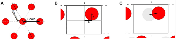
Figure 1. (A) Idealized spatial excitability pattern of a single grid cell, illustrating grid scale, and orientation. (B) Closer view of the excitability map showing the boundaries of a single rectangular tile. The phase of one cell is illustrated as x and y offsets from the center. If this were from a rigid module, each cell in the module would have a single excitability bump within the tile. (C) The offset vector connecting the centers of two grid bumps within a tile.

Although there is no direct evidence of the contribution of grid cells to place cells or navigation, the connectivity and firing patterns suggest several functions. First, layer II of the medial entorhinal cortex, where the greatest concentration of grid cells is found, projects directly to place cells in CA3 as well as indirectly to both CA3 and CA1 by way of the perforant path. This suggests that the spatial firing of grid cells may serve as input to place cells (O’Keefe and Burgess, 2005; Solstad et al., 2006). Second, the regular patterns of grid cell firing, where one bump location predicts the direction and distance to other bump locations, suggests that grid cells, at least in part, are driven by path integration (O’Keefe and Burgess, 2005; McNaughton et al., 2006). Third, the stability of grid cell firing patterns within and across sessions suggests that grid cell firing is also partially controlled by location-specific sensory cues (Hafting et al., 2005). Finally, the regular geometric firing patterns, characterized by straight lines and consistent angles, suggest that the metrics of distance and direction are extractable features (Jeffery and Burgess, 2006).

The focus of the current study is to investigate potential mechanisms where the metric properties of grid cells could be used to predict locations directly ahead of the animal’s nose: that is, the set of locations the animal would encounter if it walked on a direct path straight ahead. We call this process “linear look-ahead.” We will explore how linear look-ahead can update an animal’s location on the grid cell map to an adjacent location ahead of its nose, and how this process can be extrapolated to more distant locations, a process that can be exploited for selecting optimal straight line paths for navigation (Figure 2).

FIGURE 2

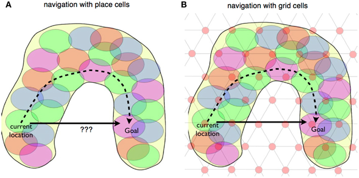
Figure 2. Place cell and grid cell navigation. (A) An idealized U-shaped spatial terrain, covered with the firing fields of place cells. Many navigation models rely on the hippocampus computing a path between current location and goal that involves crossing a minimal number of firing fields, illustrated by the dashed arrow. (B) The terrain is overlaid with an idealized grid cell firing pattern, illustrating that grid cells, in principal contain information for a linear, shortest-path route between start location and goal. The path can cross unvisited space.

Three Critical Features

Three features of entorhinal cortex need to be elaborated before proceeding with the analysis. The first is that grid cells are not the only spatially tuned entorhinal neurons. Complementing grid cells found predominantly in layer II are conjunctive cells found predominantly in layer III (Sargolini et al., 2006). Like grid cells, conjunctive cells fire in the pattern of a regular triangular lattice. In contrast to grid cells, however, conjunctive cell firing is modulated by head-direction. An individual conjunctive cell will exhibit the spatial firing pattern of a grid cell, but, additionally, while the rat is in the location of the cell’s firing bump, the cell will only fire if the rat’s nose is pointed in the cell’s preferred direction.

The second feature that is critical to our analysis is the dorsal-to-ventral increase in grid scale originally reported by Hafting et al. (2005). The scaling increase has been supported in subsequent work, and correlates both with differences in the membrane properties of grid cells (Sargolini et al., 2006; Giocomo et al., 2007) and differences in the scale of place cells at corresponding depths (Kjelstrup et al., 2008). The range of dorsal-to-ventral scale increase appears to be greater than a factor of 2 (Barry et al., 2007) but is presently unclear.

The third critical feature is the modular organization of grid cells. A grid cell module is a localized region where all cells share identical orientation and scale. That is, the characterization of individual grid cells within a module is determined solely by phase (x, y offset of grid bumps). Hafting et al. (2005), in the initial grid cell study, reported that all grid cells recorded from a single tetrode had identical scale and modular properties. Barry et al. (2007) found discrete jumps in grid scale when driving electrodes from dorsal-to-ventral, suggesting large, discrete modules. The Moser group has preliminary evidence supporting large-scale modules (Stensola et al., 2011). It appears that medial entorhinal cortex is organized as a stack of horizontal slices, with each slice representing a module, and neighboring modules representing large steps in grid scale. Our presumption is that modules are real. Although evidence for modules has only been presented for grid cells, we will also assume that the layer III conjunctive cells have a modular organization that corresponds to the overlying grid cell module (predominantly found in layer II).

This paper is organized in three parts. The first is devoted to a concept we refer to as “rigid modules.” Rigid modules are modules where the constraints of fixed grid scale and orientation are extremely tight. A “tile” is defined for a rigid module as a spatial region that contains a single grid bump for each neuron in the module. A tile is a repetitive unit that tessellates to cover all regions of accessible space. We will describe how understanding the organization of a tile is sufficient for understanding the collective properties of a rigid module, and how all between cell spatial firing relationships are represented in a tile. The final two parts will assume the existence of tile like organization in rigid modules. In part 2 we examine how regularities of movement may, through Hebbian synaptic plasticity, affect the connections amongst neurons in a rigid module. More specifically, we will show how Hebbian plasticity amongst conjunctive cells can produce small subsets of strong connections between-cell pairs where (a) the two cells have similar heading preferences and (b) the phases are such that the firing bump of the first cell is “upstream” to the firing bump of the second cell. Finally, in part 3, we will examine how several sets of rigid modules can, using linear look-ahead, identify a straight line path connecting the current location and a known goal, even if the path crosses unexplored regions of space.

Results

Part 1: Modular Organization and Rigid Modules

We call a module “rigid” if the orientation and scale of all of its members are identical. This strict criterion is intended to go beyond the similarity of orientation and scale in the description of modules. For example, while 5% variations in grid scale might be acceptable in a module, such a module would not be rigid. Are there true rigid modules in entorhinal cortex? There are three possibilities: (1) that the preliminary observations of horizontal slice modules are in fact rigid modules; (2) that the horizontal slice modules are not rigid and there are no rigid modules; and (3) that a single horizontal module contains several separate rigid subsets. Although we consider the answer unsettled, the model described in this manuscript makes the assumption that rigid modules exist and are the basis for information processing.

If rigid modules exist, then several interesting properties emerge. The first is that the vector connecting the nearest grid bumps of any two neurons in a rigid module is a constant. We call this vector the “shortest interbump vector” (SIV). Consider two grid cells A and B within a single rigid module (Figure 3). For all bumps of grid cell A the vector to the nearest bump of B is constant. The implication is that, if as an animal traverses space and one of its grid cells fires because the animal is at the location of one of the cell’s grid bumps, then movement in a specific direction and distance will always result in the subject being at a grid bump location of a particular grid cell. The relationship holds for all regions in a large environment, no matter which of the cell’s many grid bumps the subjects starts from. Moreover, this relationship is likely to be maintained across environments, given the observation that grid cells remap across different environments in a rigid manner, only by shifting the phase of all cells in a module by a constant amount (Fyhn et al., 2007). That is, in any environment, if cell A is firing and the rat moves a certain distance and direction it is likely that cell B will fire. Direction is determined with reference to the head-direction cell system.

FIGURE 3

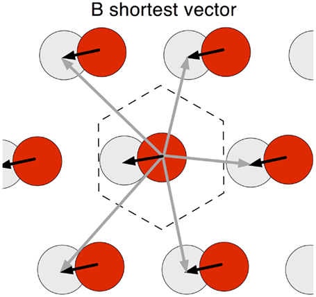
Figure 3. Shortest interbump vector (SIV). In a rigid module, the vectors connecting the bump of a grid cell to the activity bumps of a second cell are fixed. The figure illustrates the activity pattern of a single grid cell (red) with a bump in the center, and the vectors to activity bumps of a second grid cell (gray). For the central red bump – and any red bump – there are six vectors to the nearest six bumps of the gray cell activity map: the shortest is black and the others are dark gray. The SIV is constant for all red cell activity bumps. A single gray bump falls within a hexagonal tile centered on the red bump.

A second property of rigid modules is a spatial pattern we will refer to as a “tile.” In the initial paper describing grid cells, the authors introduced the concept that the firing pattern of a single grid cell will tessellate across the floor of any large apparatus (Hafting et al., 2005), where “tessellation” refers to laying out a repeated spatial bump pattern called a “tile.” In a rigid module, a tessellating pattern can be described that includes all of the cells in the module. A tile for a rigid module is a contiguous region of space that contains one and only one bump from each neuron in the module. Regions that meet this condition can be laid out, edge-to-edge to cover all of accessible space (Figure 4). For any rigid grid cell set, several boundary shapes can outline a tile, including parallelograms (base = gridscale; height = 0.866 × gridscale), a rectangle (same base and height as parallelograms), and a regular hexagon (side = 0.577 × gridscale). If a shape successfully outlines a tile in one position, it will continue to define a tile through any translation (sliding x and y) without rotation, no matter the magnitude of translation within the environment.

FIGURE 4

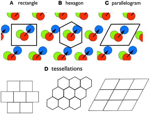
Figure 4. The tile concept. A tile is a bounded region that contains one-and-only one activity bump from each grid cell in a rigid module. A tile boundary will tessellate, in that it can be placed edge-to-edge to cover a surface. Three possible tile boundary shapes are (A) rectangles; (B) hexagons; and (C) parallelograms. (D) shows tesselation patterns. No single tile boundary will contain all of the SIVs of a rigid module, but the hexagon contains all of the SIVs connecting to a grid cell with a bump at the center.

For a given tile shape, translation changes the relationship of specific grid bumps to the boundary, but leaves tile conformity intact. Consider the firing of a rigid set of grid cells whose bumps are distributed across a large apparatus; add a boundary somewhere on this surface that defines a tile. If this boundary is lifted, translated in position and placed anywhere else, in a process similar to using a cookie cutter, the bumps enclosed in the second location will also define a tile. Although the new location changes the relationships of individual grid cell bumps to the tile boundaries, the boundary continues to enclose one-and-only one bump for each grid cell.

If we consider the interbump vectors between all bump pairs within a tile, we will find that many of these are SIVs, but, for any tile, some are longer. For example, consider bumps A and B from two different grid cells, with both lying within a rectangular tile, as in Figure 5. If bump A is adjacent to the left boundary and bump B is adjacent right boundary, the A–B distance measured within the tile will be long, approaching 1 grid bump unit. However, for each of these within-tile bumps, there is a shorter A–B vector to an outside-of-tile bump of the second cell. These shorter vectors are identical and are the SIVs for this bump cell pair. In brief, no tile will contain the SIVs connecting all of its bump pairs.

FIGURE 5

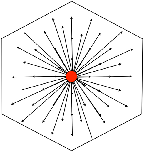
Figure 5. All of the shortest interbump vectors (SIVs) emanating from a grid bump A will describe a hexagonal tile with grid bump A at the center. The horizontal width of a hexagonal tile is the grid scale; the side length is (grid scale)/[square root (3)]; the longest SIV is (grid scale)/[square root(3)].

The set of SIVs originating from the bump of a single neuron, however, produces a surface bounded by a specific shape, the hexagon described above (Figure 5). This is a tile, since it includes one and only one grid bump for each neuron in the rigid set. Using different neurons as the origin produces translations of this tile. Thus, from the perspective of a grid bump of any grid cell, the set of SIVs extending from the bump forms a hexagon with the cell’s grid bump at the center of the hexagon. This bump-centered tile is a construct that identifies all of the SIVs for the central cell. If we consider a continuously moving animal, we can define the “current effective tile” as the hexagon in which the center represents the current location of the animal.

Firing patterns in a rigid module

The collective firing of a rigid module signals the animal’s location within a tile, but contains no other location information. A simple network of neurons in a rigid module demonstrates this property. Since the tile of a rigid module contains one firing bump of each grid cell, a tile can be used to represent the spatial firing property of each neuron. We’ll use a rigid module of grid cells, each with a grid scale of 60 cm and a rectangular tile covering 30 cm × 24 cm. Each cell’s spatial firing correlate is represented as a 2D Gaussian centered at a position within a tile. The module contains 1800 neurons, that are assigned to 100 distinct “excitability maps,” 18 neurons per map. Each excitability map covers a tile and has a single “firing bump.” The firing bumps across the set of excitability maps are spread evenly across the tile. The tile representation is tessellated to cover the floor of a 1.8 m by 1.8 m square apparatus. A virtual rat’s (vRat’s) path, moving at 25 cm/s in 10 ms steps is constructed within the floor bounds. At every time step, each neuron’s firing is calculated as a product of the vRat’s location on the neuron’s excitability map (within the current tile) and a random factor. For conjunctive cells, the vRat’s head orientation is a third factor that governs firing. The result is straightforward and as predicted. For individual time samples the firing of the set of neurons is a two-dimensional firing bump, centered on the rat’s location on a tile. As the rat moves, the center of the firing bump moves smoothly, but always remains within the tile. Figure 6 illustrates single time samples, and the accompanying video (Movie S1 in Supplementary Material) illustrates movements of the firing bump as a vRat traverses a virtual apparatus. Examining the collective firing of members of the module one could have a good estimate of the animal’s location and movement within the tile, but would have no information about which tile in the apparatus the animal occupies.

FIGURE 6

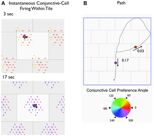
Figure 6. (A) Video frames from a movie depicting the firing of conjunctive cells in a module during a 20 s path through a rectangular chamber. (B) The 20-s path is depicted on the right. In (A), the rigid module is depicted as a rectangular tile, with each cell’s phase mapped in the surface. A virtual neuron that has fired within the previous 200 ms is depicted with others invisible. Additionally, the color (and “nose”) of the colored circle indicates the directional preference of a cell that fired. The black large circle is the virtual rat’s location at the mid-point of the 200 ms sample. Gray boxes surrounding the central tile are half-replicas of the central tile. The three things to note are (1) the firing of cells is represented by a circular cluster, centered on the rat’s location; (2) for conjunctive cells, a subset of head angles will fire together; and (3) the firing of the cells in a rigid module can only signal the rat’s location and head orientation within the module.

Part 2: Learning in Rigid Modules

A number of recent studies have proposed that grid cells are responsible for path-integration-based updates of the place cell representation of a rat’s location (O’Keefe and Burgess, 2005; Fuhs and Touretzky, 2006; Sreenivasan and Fiete, 2011). A principal goal of our research program is to see if the cells of entorhinal cortex could perform other navigational calculations. Specifically, we wanted to see if the grid-modulated cells of entorhinal cortex could perform linear look-ahead,” the process of projecting vectors to various distances directly ahead of the rat, in order to vicariously explore potential shortcuts. We speculated that linear look-ahead mechanisms might: (1) require rigid modules; and (2) be implemented by synaptic connections developed through experience-dependent plasticity.

Our reasoning is illustrated in Figure 7. Consider a rigid module of grid cells. A rat is at a particular location moving NE (45°). Firing correlates predict that one of the grid cells in the module (grid cell A) will fire and a head-direction cell tuned to 45° (HD 45) will fire. As the rat moves along this path, it will cross the firing bump of another cell (grid cell B) and it will fire. Since this is a rigid module, with fixed vectors connecting bump locations of pairs of cells, whenever the rat crosses the bump of Cell A at 45°, grid cell B will likely fire. If we imagine that these cells are connected with plastic Hebbian synapses (Grid Cell A and HD 45 → Grid Cell B), we suppose that with normal experience these synapses will strengthen. After the strengthening, we imagine that, when the rat is at the location of a firing bump of grid cell A and its nose in pointed 45°, the strengthened synapses will fire Grid Cell B, even if the rat is not moving. Grid Cell B firing along with HD 45 ought to lead to grid cell C firing, and so on, producing the sequential activation of a series of grid cells whose bumps form a straight line. This “linear chain reaction” would appear to be the linear look-ahead mechanism.

FIGURE 7

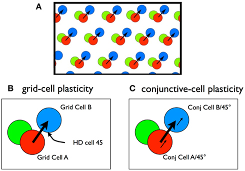
Figure 7. (A) Fixed spatial relations between the activity bumps of three grid cells in a rigid module. (B) Preliminary Hebb model. Grid Cell A + Head-direction Cell 45, firing together, will predict the firing of Grid Cell B. While this is correct, the strengthening of these synapses will not be helpful in predicting the firing of Grid Cell B. The logic requires a conjunctive firing of the two upstream cells (see text). (C) Hebb model with conjunctive cells. In this case the firing of conjunctive cell A/45° predicts the firing of conjunctive cell B/45°. If the synapse has plasticity following Hebbian rules, the synapse ought to strengthen with experience and lead to predictive firing.

The problem is that this does not work. This is because HD 45 does not selectively predict the firing of Grid Cell B (or C). Since the firing bumps of all grid cells can be approached from a 45° angle, HD 45 equally well predicts the firing of all grid cells. Similarly, Grid Cell A does not predict the firing of Grid Cell B any more than the firing of other grid cells whose firing bumps surround it. While it is true that the conjunction of Grid Cell A firing and HD 45 predicts the firing of Grid Cell B, it is only the conjunction that is predictive. Knowledge of the firing of each cell alone is of little or no predictive value. Most importantly, the Hebbian process does not signal conjunction – the Hebbian strengthening rule does a poor job as a logical AND operator. This problem is logically identical to a problem with water-maze learning described by Brown and Sharp (1995). As the authors noted, the difficulty is due to the problem of “linear separability” or the “exclusive or” (XOR) problem (Minsky and Papert, 1969). Predicting the firing of Grid Cell B requires a logical AND operator between the variables of grid cell firing and head-direction which simple rules of synaptic plasticity cannot provide. Below we use a simulation to show that applying a Hebbian learning rule between pairs of connected grid cells does not produce useful or selective patterns of synaptic strengthening.

The failure of useful association can be seen in a simulation. The simulation models a rat making a 1-h virtual path across 1.8 m × 1.8 m space. The path is created by having the rat move at constant speed (20 cm/s) and sampling at 10 ms intervals. At each sample the rat’s heading direction is changed from the previous direction by a small random factor, within the range ±3°. When the rat encounters a wall, its heading changes in a random direction within accessible space.

The simulation involves a single grid cell that receives inputs from a large number of grid cells and head-direction cells. If we think of the single grid cell as “Grid Cell B” the useful association question boils down to whether during an extended random-walk training session we will see evidence of correlation between the firing of any of the upstream grid cells or head-direction cells and this cell. If Hebbian plasticity were in place, such correlated firing would lead to selectively strengthened synapses that in turn, might produce useful patterns of connection. In the simulation one group of afferents is a set of 882 grid cells with 49 distinct excitability maps whose peaks are evenly distributed over the tile. The second group of afferents is a set of 882 afferent head-direction cells with 18 distinct heading preferences, distributed in 20° increments. The firing of each afferent neuron and the single downstream neuron is determined for each 10 ms interval during the 1-h path. Firing of each grid cell is determined as a function of three factors: (1) the vRat’s location in the cell’s excitability map; (2) a random factor; and (3) a grid cell threshold factor (to achieve a mean firing rate of about 5 spikes/s). Firing of each head-direction cell is determined by (1) the vRat’s heading direction relative to the cell’s preferred direction; (2) a random factor; and (3) a head-direction threshold factor.

Each of the afferent cells has a connection to the target cell. For each connection the afferent cell is termed the “origin” and the single downstream cell is the “termination.” To assess the correlated firing between the cells at each end of a connection, “hits” and “misses” were tabulated following each target cell spike. A hit was tabulated when the upstream cell fires within a 500 ms window preceding the downstream spike; a miss was recorded if there was no spike in the time window. At the conclusion of the 1-h path a hit ratio was calculated for each connection (e.g., between each pair of cells).

$\text{Hit Ratio}=\text{hits}∕\left(\text{hits}+\text{misses}\right)$

The results reveal little-to-no evidence that Hebbian mechanisms could contribute to look-ahead or other aspects of anticipatory firing. High hit ratios indicate co-active firing between the upstream cells and the single downstream grid cell. If there was a subset of connections with enhanced hit ratios, this would indicate, at least in principle, that selected synaptic connections could be strengthened by experience-dependent Hebbian mechanisms. The results are shown in Figure 8. The overall finding is that selective high hit ratios are barely present. There is a small tendency to observe high hit ratios for connections between grid cells with peak excitability maps in the region surrounding the peak excitability of the target grid cell. There is no tendency for high hit ratios among subsets of head-direction cells. In brief, high hit ratios, which, if Hebbian mechanisms were in place would lead to synaptic strengthening, could not lead to a linear look-ahead mechanism suggested above and in Figure 8. The reason for this is clear. The prediction made by Figure 7 is that the conjoint firing of Grid Cell 1 and HD 45 predict the firing of grid cell 2. There is no suggestion that the firing of either of these cells alone will predict the firing of grid cell 2. The simulation shows that neither the firing of Grid Cell 1 nor HD 45 in isolation – or any grid cell or head-direction cell – will be of substantial predictive value.

FIGURE 8

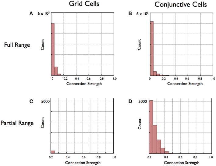
Figure 8. Histograms of results for connection strengths (co-activity indices) between all cell pairs in a rigid grid cell module (A,C) and conjunctive cell module (B,D). (A,B) show that for both Grid Cells and Conjunctive cells that great majority of scores are low, roughly 80% of the strengths falling in the lowest bin. In (C,D) high-strength scores are selectively examined by eliminating values below 0.2 and rescaling. This close examination reveals a subset of strong connections found between pairs of conjunctive cells (D) but not grid cells (C).

The conjunctive cell solution

The difficulty in using Hebbian rules to create networks that anticipate future locations is that anticipatory prediction requires a logical conjunction of grid cell firing and head-direction firing – a logical AND relation. Simple Hebbian learning rules cannot perform a conjunctive association. One solution might be a complex multi-compartmental synaptic morphology, that could perform logical AND operations (Alarcon et al., 2006). We considered the possibilities of patterned inputs to synaptic spines, or carefully arranged patterns of axo-axonic inputs. While exotic and un-documented patterns of neuronal connection might solve the “conjunctive” problem, a more parsimonious solution is known to exist in entorhinal cortex: conjunctive cells. Although we do not know how conjunctive cells acquire their basic firing properties, it is clear that they perform the conjunctive operation. A given conjunctive cell fires as if it is an AND gate for a head-direction cell and a grid cell. It will fire in a grid-like spatial pattern, but only when rat’s head is pointed in the preferred direction (Figure 7C).

For the remainder of this paper we will examine the role of conjunctive cells in two steps. First, we will simulate a training session, where a vRat moves randomly through space, to show that the pattern of correlated firing between pairs of cells is precisely what is predicted above. In Part 3 we will use the strengthened connections to produce a series of activations simulating linear look-ahead.

Synaptic strengthening in conjunctive cells

The simulation aimed at looking for patterns of synaptic strengthening was run separately on sets of conjunctive cells and grid cells in rigid modules. Each module contained 1800 all-to-all connected neurons (3,240,000 connections). The grid cell rigid module contained cells with 100 separate excitability maps, whose peaks were evenly spread across the tile. Eighteen grid cells shared a single excitability map. Their firing was individuated by the random excitability factor (0–1.0) for each cell at each time step along the path. Each conjunctive cell had a unique phase/heading preference combination. Each conjunctive cells was assigned 1 out of 100 phases (excitability maps) and one out of 18 evenly spaced heading preferences. At each 10 ms step, as the vRat moved along its path, the firing of a conjunctive cell was determined by phase, heading preference and a random factor. Connections between all pairs of grid cells and conjunctive cells were created.

The simulation was run using a single 30-min path with firing of each cell determined at each 10 ms interval. Although the conjunctive cell module and the grid cell module were run separately, both simulations were run on the same path, with identical input parameters. “Hits” and “misses” for each connection were updated during the run; at the end of the run “hit ratio” was computed for each connection.

The question these simulations investigated was whether specific patterns of correlated firing between pre- and post-synaptic cells develop within either rigid module. As before, we used the hit ratio from each cell pair connection to estimate co-active firing between cell pairs. High hit ratios are exclusively found in the conjunctive cell module, and, even there, the number of connections with high hit ratios is a small fraction of the total. As shown in the histograms of Figure 8, the great majority of connections in both the grid cell and the conjunctive cell modules have low hit ratios. If the higher end of the histograms are examined (Figures 8C,D apply a 0.2 strength cut-off), it is clear that virtually all of the high hit ratios, those above 0.2, are from the conjunctive cell modules. A chi-square test of the difference in proportion scores above 0.2 is significant at the 0.01 level.

Next we looked for distinctive features in the subset of conjunctive-to-conjunctive connections with high hit ratios. Since the vRat tended to move in straight lines, creating sequential firing of conjunctive cells with similar heading preferences, we examined the difference in heading preference in the origin and termination cells for each cell pair. Figure 9 is a polar scatter plot of hit ratio as a function of the heading preference difference. As predicted, cell pairs with highly correlated activity (e.g., hit ratios above 0.2) were exclusively the cell pairs with close match in preferred headings.

FIGURE 9

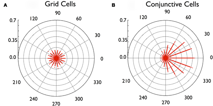
Figure 9. Circular scatter plots of connection strength as a function of the difference in heading preference of the connected cells. (A) plots connection strengths between pairs of grid cells, where all values are low, and unmodulated by (pseudo) heading preference. (B) plots connection strengths between pairs of conjunctive cells, where high values are found between pairs with similar heading preference (i.e., difference values near zero).

Connection strength maps help to further identify the small set of strong connections among conjunctive cells (Figure 10). These maps are limited to connections between pairs of neurons with identical heading preferences. To construct the map, a single “origin” cell is placed at the center, and the co-activation score is displayed as a black circle, displaced from the center by the SIV between the two cells. With the size of each circle representing the co-activation score, the set of circles sits on a hexagonal tile, with the “origin” cell at the center. From the maps we see two further features of the connections with high scores. First, high-score connections are greatest for neurons with neighboring firing bumps (short SIVs). Second, the highest co-activation scores are found “downstream” to the origin cell; that is, with the center as origin, in the direction of the heading preference of both cells. This would be the most frequent direction of the vRat’s movement.

FIGURE 10

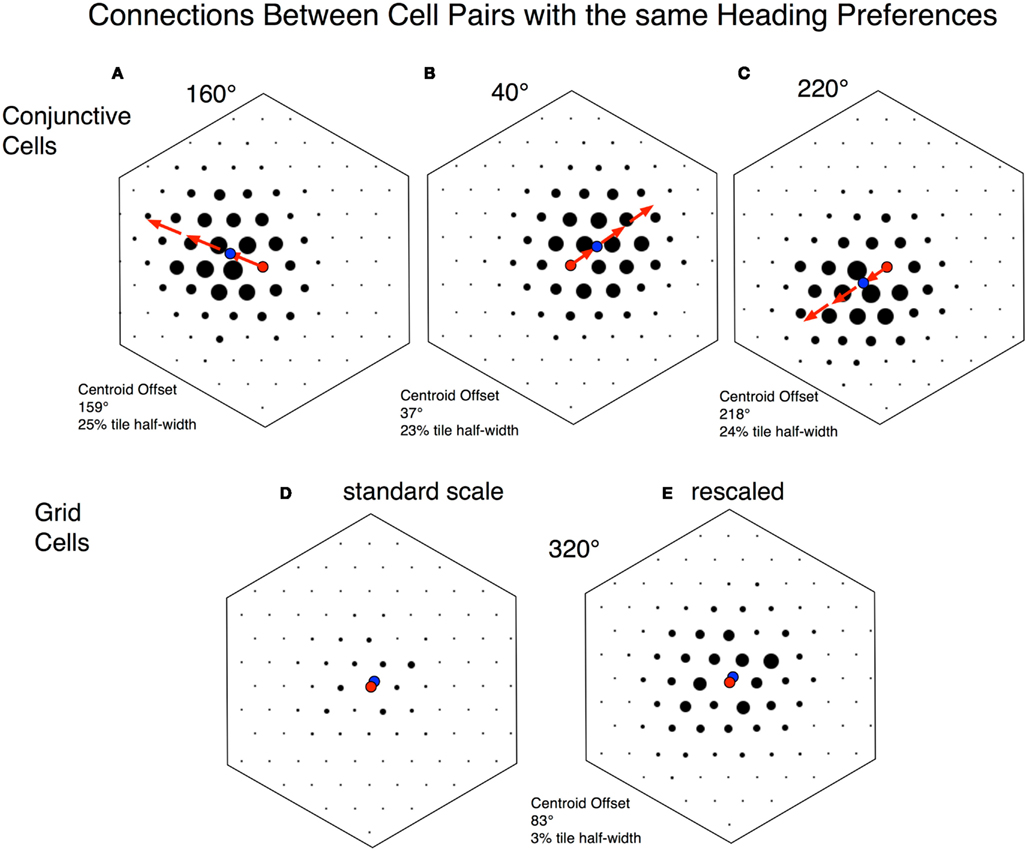
Figure 10. Connection strength plots. Each plot represents a conjunctive cell or grid cell tile with a single cell at the center, represented by a red circle. Surrounding dots represent connections from the central neuron to other neurons, with the strength of connection depicted by the size of the circle. The location of each circle represents the shortest interbump vector (SIV; or phase difference) between the central neuron and other depicted neurons. For conjunctive cells, all of the neurons depicted share the same heading preference. These plots come from rigid modules with 100 evenly spaced phases, with a single cell at each phase location. As noted above (Figure 5) since we are plotting the set of SIVs from a single cell, the surface described is a hexagon. Note that each plot represents a very small subset of total connections in a rigid module. In these examples 100 connections out of a total of 3,238,200 connections are shown. The connections are restricted to those: (1) with a particular cell as an origin (out of 1800) and (2) with terminations on cells with the same heading preference (out of 18 at each phase location). The plots selected are representative out of 1800 alternatives. The top three panels (A–C) are from a simulated 30 min session with 1800 conjunctive cells distributed across 100 phases with 18 heading preferences at each phase. The bottom two panels (D,E) are from a simulated 30 min session with 1800 grid cells in a rigid module. These cells were distributed across 100 phases. For each phase location, 18 arbitrary directional identifiers were assigned that had no influence on the cell’s behavior. (A–C) are plots from origin cells with heading preferences of 160°, 40°, and 220° respectively. The noteworthy feature of each plot is that the density of strong connections is near the center, but displaced from the center. The direction and distance of displacement is calculated by computing a centroid (center of mass) for the connections (blue dot). The distance of centroid displacement was ∼25% of the maximal distance to the edge of the hexagon. The direction of displacement for all three plots is very close to the direction of the common heading preference for the conjunctive cells. (D) Is a similar plot from a single grid cell. The directional preference is an arbitrary assignment made to each cell and does not reflect firing preferences. The point to note is that all of the connection strengths (black circles) are low. (E) Is a remapping of the same data, but increasing the dot-scale by a factor of three. This shows that relatively stronger connections are close to the central cell. Both panels show that the magnitude of displacement of centroid from center is almost imperceptible.

The pattern on each map can be quantified by calculating the vector from the center of the tile to the centroid of the weighted connections (see Materials and Methods). When this is done for all 1800 maps, the mean difference between heading preference and centroid vectors is 0.3°, with a mean absolute value of 7.3° (Figure 11A). Doing the same computation on grid cells (with heading preference randomly assigned) or a pure Monte Carlo distribution of 1800 angle pairs results in mean absolute deviations of ∼90°, the mean chance difference between two randomly selected angles (Figures 11B,C).

FIGURE 11

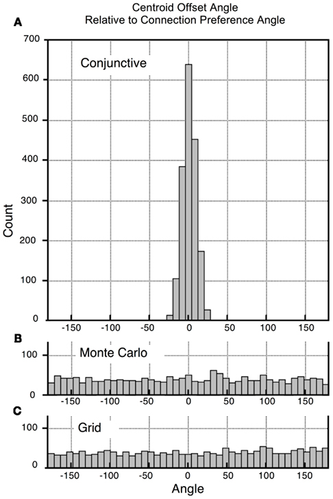
Figure 11. Histograms of centroid offset angles for all cells in a simulation. Recall that Figure 10 illustrates that the displacement centroid for 3 groups of connections are in the direction of the common heading preference of the cells. To prepare this figure similar centroid offset calculations were made for all 1800 possible subsets. Each centroid-offset-angle was subtracted from the common heading preference and the results plotted as a histogram. As predicted, common heading preference and offset angle are very similar. (A) For the conjunctive cell module, the angle difference clustered around 0, with a maximal deviation of 27°. Mean unsigned deviation was 6.7°. (B,C) Perform similar calculations on Monte Carlo simulations of direction pairs (B) and grid cell pairs where heading preference was randomly assigned. For each of these “random” simulations produced flat distributions, with deviations from 0 averaging ∼90°.

The connection strength maps of Figure 10 show a clear spatial pattern of high co-activity scores. It is clear that the pattern of high hit ratios for conjunctive cells is proximate to the rat’s current location and “points” downstream, in the direction that the rat is heading. We conclude that high hit ratios are found exclusively in a subset of connections among conjunctive cells. These connections share three properties: (1) they connect conjunctive cells with identical or similar heading preferences, (2) they connect conjunctive cells with nearby spatial excitability peaks, and (3) they connect origin conjunctive cells with cells whose excitability peak is in the direction the rat is facing.

Time window and the learning rule

The hit ratio learning rule is a form of Hebbian association, in that the hit ratio will be high when pre-synaptic firing “predicts” a post-synaptic spike. Hit ratio computations perform almost exactly as a binomial correlation. When correlation 1 (a binomial correlation between presynaptic cell firing in a time window and post-synaptic firing) was computed for three sessions the correlations between the correlation 1 and hit ratio scores were 0.992, 0.994, and 0.992. We have used a long (500 ms) pre-synaptic window in most analyses in order to observe the overall pattern of interaction. Physiological data suggests shorter window times, in the order of 50 ms, may be more appropriate for LTP (Bi and Poo, 1998). Shorter windows have two effects on patterns of synaptic strengthening: the error of angular estimation increases and the distance offset decreases (Figure 12). Although the selective enhancement in the direction of heading preference decreases, after a 60 min training session, directionally selective enhancement remains statistically significant down to 50 ms. Finally, we implemented a form of spike-time dependent plasticity (STDP), with two temporal firing windows: an enhancement window, if firing preceded the post-synaptic spike, and a decrement window if pre-synaptic firing followed the post-synaptic spike (Bi and Poo, 1998). STDP enhances the sensitivity of conjunctive cells to look-ahead plasticity, both in terms of the minimum time window for effective plasticity and the length of the downstream displacement.

FIGURE 12

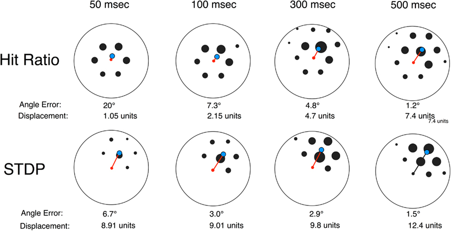
Figure 12. Effects of pre-synaptic spike window and spike-time dependent plasticity (STDP) patterns on connection strength. The top row uses the hit ratio synaptic weighting method while the bottom row uses a STDP method. All plots are for an identical 60 min Training session. The preference angle for all cells is 60°, so a perfect displacement will be at a 60° angle from center. Each plot depicts the centroid (center of mass) for the strength of connection between one neuron and 48 other neurons with the same heading preference (60°). The set of depicted weightings for each plot is truncated to a circle, and cells with connection strengths below a threshold are not displayed. The central cell is a red dot, and the centroid is a blue circle. For this representative set, the angle of centroid offset improves with greater pre-synaptic integration time, but all are less than chance (90°). The distance of centroid displacement also increases with integration time. The second row depicts the connection strengths of the same neuron pairs, where strength is a produced by a spike-time dependent plasticity rule (LTP–LDP). With a STDP learning rule errors are generally smaller, centroid displacement distances are larger, and are less affected by integration time.

Part 3: Linear Look-Ahead with Conjunctive Cells

In Part 2 we established high pre-to-post-synaptic correlations between the firing of pairs of conjunctive cells whose SIVs point in the direction the rat is facing. The final question we will address is whether transforming these firing correlates, via Hebbian mechanisms, to synaptic strength is sufficient to produce linear look-ahead. Specifically, we activate a set of conjunctive cells as if a rat is in a fixed location and head-direction and see if this sets up a step-by-step activation of conjunctive cell cohorts (F groups) that represent a linear sequence in the direction the rat is facing. There are four steps to the simulation. First, the hit ratios calculated during training (Part 2, above) are transformed into “connection strengths.” Second, the vRat is placed at an arbitrary location in the environment with a particular head orientation, and the corresponding subset of the location and directionally tuned cells activated (firing set F1). Third, the cells that fire in F1 activate their outflow connections. Fourth, each downstream cell summates the F1 inputs to produce a level of excitation. Fifth, the downstream cells are rank-ordered by their excitation state, with the top X% (typically 2%) set to fire (F2). This process is iterated, with each iteration producing a subsequently activated cohort of neurons (F2, F3, etc.). The prediction is that each cohort of firing neurons will form a circular cluster, with the centroid of the cluster proceeding in a step-wise manner in the direction of the initial head orientation. A confirmation of this prediction is illustrated in Figure 13. A series of six step activations is illustrated. In each the set of activated conjunctive cells forms a neat circle with a centroid. The progression of centroid locations produces a vector moving away from the start location at the angle of the initial heading direction.

FIGURE 13

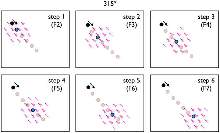
Figure 13. A trained module of 1800 conjunctive cells was tested for linear look-ahead. As described in methods, F1 is a set of conjunctive cells that fire in the rat’s initial orientation, in this case the upper left of a rectangular tile, with a head orientation of 315° (black dot). Panels labeled Steps 1 through 6 are the sets of conjunctive cells activated from the previous set of firing neurons. F2 is activated from F1 (initial conditions), F3 from F2, etc. Each violet dots represents a conjunctive cell that fires in that step, with the protruding line representing the cell’s preferred heading direction. (Multiple lines represent multiple cells). Note that for each step, the set of firing cells remains a circular cluster. The blue dot is the centroid (center of mass) of the firing cells. Faint red dots are the entire path for the six steps. It’s clear that with each step the centroid progress in the direction of head orientation.

Once F2 is activated, will it set off a chain reaction, a series of activations progressing in a straight line in the initial heading direction? The answer is a partial yes. In almost all cases, the first set of activation steps remain linear, as seen in Figure 13. In extended series, however, there can be drift, as seen in Figure 14A. Most commonly, when drift occurs, the trajectory locks in on a nearby direction. When a single training session is used, certain directions are preferred. We feel that these directional preferences are due to inhomogeneities in the 30-min training session.

FIGURE 14

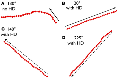
Figure 14. In panel (A) the initial position had a head orientation of 130°. For the first eight steps the centroid location progressed at approximately a 130° angle, but in subsequent steps the direction drifted and stabilized at about 180°. In (B–D) head-direction stabilization was added (see Materials and Methods). We find that with head-direction stabilization the linear look-ahead mechanism progresses continuously in the initial heading direction.

Adding a steady head-direction signal at each step is a straightforward method that appears to eliminate drift. In the experiments described above, location and head-direction inputs were turned “on” to initiate activity, but were “off” in subsequent activity steps. We feel it is reasonable to leave the head-direction signal “on” throughout the look-ahead process. This is postulating that the rat is stationary during look-ahead, with its head pointed in the look-ahead-direction. Since head-direction cells maintain firing during stationary behavior (Taube et al., 1990), it seems reasonable to surmise a tonic head-direction input to the conjunctive cell module. With head-direction input maintained during each iterative step in the look-ahead process, drift is effectively eliminated. This is illustrated in Figures 14B–D where an unchanging head-direction factor was added to the summed excitation at each step. In each case, trajectories remained steady for up to 40 steps. We conclude that a tonic head-direction input may be essential for the look-ahead process.

Discussion

Before discussing the implications of the current work, we would like to address some of the limitations and qualifications. First, the model is based on imagined connections among conjunctive cells and between grid cells and conjunctive cells. As noted above, there is very little experimental work addressing connectivity within and across layers of entorhinal cortex. For example, there is no definitive evidence for layer II stellate cell to layer III pyramidal cell connections (grid cell to conjunctive cell) nor is there evidence for-or-against conjunctive cell to conjunctive cell connections. Although each of these connections seems likely, experimental work is needed.

Second, it should be clear that this model performs “linear look-ahead” for a single rigid grid cell module. Since, as we have described, each rigid module is tiled across accessible space, the result of each step in the linear look-ahead process is not unique; rather, each step identifies a number of locations corresponding to the number of tiles. Unique locations can be identified if linear look-ahead is performed synchronously across several modules with different grid scales. We are in the process of doing this work.

Third, most of the simulations done for this paper were done with integration times of 500 ms, far longer than the estimated 50 ms pre-spike integration time for LTP. Shorter pre-spike integration time windows work, but with decreasing apparent effectiveness. Preliminary tests with a combination of a pre-spike LTP window and a post-spike LTD window (STDP) suggest these may be essential for look-ahead plasticity with realistic (shorter) integration times. It is important to note that Zhou et al. (2005) have shown both LTP and LTD in slice preparations of entorhinal layer II/III pyramidal neurons.

Finally, It should be noted that the notion of “linear look-ahead” is not unique to our work and may be effected through other mechanisms. Specifically, Erdem and Hasselmo (2012) have devised a “linear look-ahead” model based on the phase-interference mechanisms of entorhinal grid cells, with no involvement of conjunctive cells. The Erdem and Hasselmo model can solve complex navigational problems, such as taking shortcuts and dealing with detours. An interesting similarity is that both models require continual head-direction cell firing for optimal operation. We note that the two mechanisms are not in conflict and may operate separately or together to add to navigational prowess. In addition, Navratilova et al. (2012) explore the possibility that conjunctive cell inputs to grid cells and hippocampal place cells produce the “look-ahead” component of phase precession. In line with our thinking, the authors of each of these studies propose an entorhinal-based look-ahead process as a mechanism for anticipating future locations.

The motivation for this work was an effort, stated in a previous paper, to find mechanisms for computing vectors – straight line paths – between an animal’s current location and a previously visited goal (Kubie and Fenton, 2009). The constraints were that the animal must have performed journeys connecting these two locations, but the animal need not have visited locations along the direct path. Figure 2 (modified from a figure in the earlier paper) represents these constraints, and shows how a vector-navigational system could, in principle take efficient paths across unvisited regions of space. The vector-navigation system hypothesized in the Kubie and Fenton (2009) model relied on path integration and speculated that such a mechanism might reside in entorhinal cortex. The current study explores the possibilities of vector-based navigation among known neuronal types in entorhinal cortex. With only two key additional assumptions, specifically that grid-like cells are organized in rigid modules and that the synaptic connections within a module are established in accord with Hebbian learning rules, we explored how grid cells and conjunctive cells could produce a mechanism termed “linear look-ahead.” The reason for this is that the regular arrangement of grid cell and conjunctive cell firing bumps implicitly fills unvisited regions of space with predicted firing patterns. Figure 2 illustrates a spatial pattern that covers both visited and unvisited regions of space. Implicit is that both grid cells and conjunctive cells have predicted firing properties as animal first explores, or vicariously explores, unvisited regions of space.

Exploiting linear look-ahead, an animal can, in principle, sit in one spot and take a hypothetical path across unvisited regions of space in search of goals. The process might go something like this. The animal sits in one region of space with a goal, represented by place cell activation and an associated sensory input also activated. In the start location the rat can explore potential direct paths to the goal. Through the process of linear look-ahead it can activate a series of conjunctive cells, grid cells, and place cells to see if any of the patterns matches the goal pattern. If a goal match is found in the look-ahead process then the current state of “look-ahead” would represent the direct path to the goal. In brief, the linear look-ahead process implemented in conjunctive cells is a viable candidate for vector-based navigation.

Figure 15 is a simplified schema of layers 2 and 3 of entorhinal cortex illustrating how these two cell types might interact. According to this scheme:

1. Grid cells (predominantly layer II) and conjunctive cells (layer III) have reciprocal connections, such that there are corresponding grid cell/conjunctive cell sets. “Descending” and “ascending” connections can be activated independently (as far as we know, reciprocal connections have not been physiologically established, although cell morphology makes the connections likely (Lorente deNo, 1933; Canto et al., 2008).

2. Conjunctive cells have network processing that can produce linear look-ahead.

3. Grid cells have (indirect) reciprocal interactions with hippocampal place cells such that grid cells can update place cell firing and sensory information from place cells can update grid cell firing (van Strien et al., 2009).

4. Each of these connection sets is gated. That is, connection sets can be turned off or on such that some processes can operate without the interference of others.

FIGURE 15

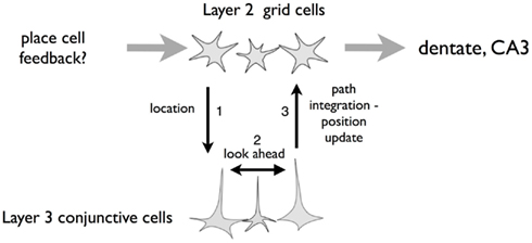
Figure 15. Schematic of grid cells (layer 2 EC) and conjunctive cells (layer 3 EC). We hypothesize vertical integration and interaction between overlying layer 2 grid cells and deeper layer 3 conjunctive cells. Additionally, the conjunctive cells are interconnected to provide the “linear look-ahead” described in the paper. Each of the arrows can operate independently. The grid cell projection to conjunctive cells “sets up” the conjunctive cells to be in register with grid cells and sensory cues from the environment. If this influence is reduced and inter conjunctive cell interaction turned on (along with head-direction input) the conjunctive cell layer can process linear look-ahead, to predict locations ahead of the animal’s nose. Finally, the conjunctive cell layer projects to the grid cell layer, permitting the grid cells to reflect the look-ahead mechanism. We see three functions of linear look-ahead. First, the mechanism can do long-distance look-ahead while the animal is stationary to predict distance locations. Second, the mechanism can do short-distance look-ahead, providing continual update while the rat is in motion. Finally, the mechanism can add to the cohesion of both conjunctive cells and grid cells, making a rigid network even more rigid.

With this scheme in mind, we can envision several functions for linear look-ahead. First, “long-distance” linear look-ahead, as described above, would be described as: (1) initial activation of conjunctive cells from grid cells at the start location followed by a disconnection (arrow 1); (2) simultaneous activation of conjunctive cell linear look-ahead (arrow 2); and the conjunctive-to-grid cell connection (arrow 3) to look for a match at the goal.

“Short-distance linear look-ahead” might be the mechanism for continuously updating the conjunctive cell/grid cell representation during active navigation. According to this notion, during navigation, when there is a velocity signal, there is a constant cycle of arrows 1, 2, and 3 in Figure 15. The grid cells representing the rat’s current location (which may be reinforced by sensory cues) excite a corresponding set of conjunctive cells; (2) conjunctive cells trigger a set of “downstream” conjunctive cells in advance of the animal’s current location on its path; (3) the “downstream” conjunctive set excites the corresponding “downstream” set of grid cells. In support of this notion is the stationary property of attractor networks. Several authors have noted that if the grid cell networks functions as an attractor system it require an external drive to update during locomotion (McNaughton et al., 2006; Giocomo et al., 2011; Sreenivasan and Fiete, 2011). An asymmetrical input, such as provided by conjunctive cells, could provide that drive.

A third function is that linear look-ahead might contribute to establishing and maintaining the rigidity of grid cell and conjunctive cell modules. In creating patterns of synaptic strengthening among conjunctive cells, we assumed a priori rigid modules. What if the modules were initially only slightly rigid? We imagine that it might take extensive experience for sufficient co-incidence of the firing patterns for rigidity to emerge based on Hebbian learning rules, but nonetheless the patterns would still emerge (Langston et al., 2010; Wills et al., 2010). After synaptic strengthening occurs, the short-distance linear look-ahead mechanism will reinforce rigid relationships among conjunctive cells. Even partially implemented linear look-ahead will reinforce the SIV patterns of neighborliness and direction. This will, in turn, strengthen conjunctive cell mediated linear look-ahead.

In summary, linear look-ahead operating within the hippocampal formation may have utility at three distinct spatio-temporal scales. First, the long spatial and temporal time scales are in accord with our goal of understanding how linear look-ahead could be implemented to navigate environments with unfamiliar expanses. Second, on the shorter scales of the next locomotor steps, linear look-ahead may provide a means for overcoming representational inertia by updating the representation as the animal moves through space. The third scale is that of synaptic plasticity and may be most relevant for the development of grid-like cell modules. Beyond our initial intent, linear look-ahead may have fundamental importance to the operations of the spatial representation system.

Methods

Grid Cells and Conjunctive Cells

The computational method is organized around a set, or sets, of neurons in a rigid module. The end result is that the program produces an excitability map for each grid cell or conjunctive cell that covers the surface of the apparatus. Grid bump size, grid scale, and grid orientation can be varied. Excitability maps are organized around the tile. Although a number of tile shapes are equivalent (parallelogram, rectangle, hexagon) the program uses a rectangular tile with a 0.86 × 1.0 aspect ratio. Grid scale sets the width of the tile. Grid cell distribution is the number of distinct phases per tile, with each phase occupying a single unique tile position. In the current study, phases were evenly distributed across the tile surface in 49 (7 × 7), 64 (8 × 8), or 100 (10 × 10) locations. For a given neuron, phase can be thought of as a rectangular tile with a dot at the phase location.

A single “bump surface” is used for all excitability maps in a simulation. This surface is a 2D Gaussian with a value 1.0 at center that drops to a cut-off at 0.05. The fall-off rate of the Gaussian determines the size of grid bumps.

A neuron’s excitability map is created in two steps. First, the tile with the neuron’s phase is tessellated across the surface of the apparatus; the tessellation pattern has alternate rows offset by half the tile width creating a “brick wall” of the rectangular tile pattern (Figure 4A). Next, the “bump surface” is repeatedly added, centered on the phase location of each tile. The resulting excitability map resembles a smooth grid cell rate map. Values vary from 1.0 at bump centers to 0 between bumps.

Each conjunctive cell, in addition to having an excitability map, has a preferred heading direction. Typically, preferred heading directions are grouped in 20° bins, but all directions are possible.

Paths are computed in a virtual rectangular enclosure 1.8 m × 1.8 m. The enclosure is divided into 25600 × 25600 square pixels with sides of 0.7 mm. Virtual rats move at a constant running speed of 20 cm/s. The vRat’s location is sampled at 10 ms, making each step 28 pixels in the vRat’s current direction. After each step current direction is updated by a random factor ranging between +3°. When the vRat encounters a wall, direction is updated as a random direction that takes the rat to a position within the apparatus.

During path execution the firing of grid cells, conjunctive cells, and head-direction cells is updated with each virtual step, based on the rat’s location and head-direction. For a grid cell, firing is determined by an excitation equation:

$\text{Excitation}=\text{excitability}\left(x,y\right)\times \text{RF}$

where

x and y are the rat’s location

excitability() = the apparatus excitability map for that cell

RF = a uniform random value between 0 and 1.0

    A grid cell fires if

$\text{Excitation > GridCellThreshold}$

where GridCellThreshold is a value set to obtain a mean firing rate of 5 AP/s for grid cells.

For conjugate cells, an additional factor, the “heading direction factor” (HDfactor) is also computed.

$a^{\prime }=\left|\text{CurrentHeadingAngle}-\text{Heading}\text{PrefenceAngle}\right|$

hw = “heading width”: changes the width of the curve. Default is 0.5.

HDfactor – heading direction factor is a value ranging from 0 to 1

if(a′/hw) > 180 then HDfactor = 0 else

HDfactor = cos(a′/hw + 1)/2

With a “heading width” (hw) of 0.5 the cosine fall-off will reach zero 90° from peak. Lower hw values create sharper tuning curves.

Adding the HDfactor to the excitation equation:

$\text{Excitation}=\text{excitability}\left(x,y\right)\times \text{RF}\times \text{HDfactor}$

where HDfactor is computed as defined above.

a conjunctive cell fires if

$\text{Excitation} > \text{ConjCellThreshold}$

where ConjCellThreshold is a value set to obtain a mean firing rate of 5 AP/s.

Finally, head-direction cell firing is computed identically to conjunctive cells, but without an excitability map.

Connections are objects that connect neurons. A connection has an “origin” cell and a “termination” cell. A connection can also store values of “hits” and “misses.” During path execution, when a cell fires, all of the connections that have the cell as a “termination” are queried. If the origin cell has fired within the set time window (typically 500 ms) the hits value is incremented; if the origin cell did not fire within the time window, the connection’s misses parameter is incremented. In simulations, all cells of a module are connected; therefore, if there are 882 Grid Cells (49 phase locations; 18 cells per location), there are 777,924 connections. During training sessions, connections do not influence neuronal firing; they simply collect information. A connection with a high hit ratio [hits/(hits + misses)] has high correlated firing. If Hebbian learning rules are applied, connections with high hit ratios will be strengthened.

Connections are depicted in hit ratio maps. Hit ratio maps have a single cell at center and connections depicted spreading from the center. The distribution of connections is determined by the SIV from center cell to the connected cell. The surface formed by the set of these connections is a hexagonal tile. (This is because the set of SIVs from a single cell is a hexagonal tile with the cell at center). The magnitude of the hit ratio is depicted as the radius of a circle. For conjunctive cells hit ratio maps are typically limited to the set of conjunctive cells sharing a single directional preference. For grid cells, the distribution of connections can be made for a single grid cell, for each SIV, or as the average of identical SIVs emanating from the central cell.

Three methods have been used for computing connection strengths: Hit ratio, Correlation 1, and a STDP (spike-timing dependent plasticity). The hit ratio method is as described above. The computed hit ratio for a connection is used as connection strength. Correlation 1 is a binomial correlation between the firing of the pre-synaptic cell in the pre-spike-time window and the firing of the post-synaptic cell. (Empirically, the correlation between Correlation 1 and hit ratio is consistently above 0.99). To compute the STDP value we calculate Correlation 2, a correlation between the firing of pre-synaptic cell in a time window after the post-synaptic cell fires. STDP for a given connection is (Correlation 1–Correlation 2). The STDP measure is conceptually equivalent to LTP–LTD, for a given synapse, where the LTP and LTD time windows have identical length (Bi and Poo, 1998).

After training sessions have been completed, connections can be turned on and used to drive conjunctive cells. Two methods have been used. The first is a conjunctive cell-only mechanism.

1. Initial state. A vRat with a set of conjunctive cells is placed in a location in the environment with its head pointing in a particular direction. Using the mechanism described above, the set of conjunctive cells that fire is determined. A “set of firing cells” is called a firing set (FS). This first set is FS(1).

2. cyclic firing

    a. The connections that have FS(1) as origin are queried. For each of these, the strength of the hit ratio is added to a value in the termination cell called “excitation.”

    b. The cells in the module are sorted based on their stored “excitation value.”

    c. The top 2% of cells with highest excitation values are set to fire. The threshold value is typically 3%. These become the next set of firing cells [FS(2)].

    d. All excitations are reset to 0 and the process is repeated, starting at 2a, with FS(n + 1) replacing FS(n).

The second mechanism is termed “conjunctive plus head-direction stabilization.” As the name suggests, a head-direction value is included in calculating the excitation of each cell at as part of step 2b. The head-direction factor uses the formula above for computing the deviation of head-direction preference from head-direction in the initial state.

For each step in the cycle, the vRat’s represented location is computed in a two-step process. First, the rat’s last location is taken as a first estimate. We compute the center of mass for the SIVs from the first estimated location to each cell in the current firing set and term this the “correction vector.” The computed location is the “first estimate” + the “correction vector.” This gives both the estimate of the animal’s location on the tile and in the full environment.

Conflict of Interest Statement

The authors declare that the research was conducted in the absence of any commercial or financial relationships that could be construed as a potential conflict of interest.

Acknowledgments

NIH grant R21 NS072891 to John L. Kubie contributed to the support of this work.

Supplementary Material

The Movie S1 for this article can be found online at http://www.frontiersin.org/Neural_Circuits/10.3389/fncir.2012.00020/abstract

Movie S1. video simulation of the firing from 1800 conjunctive cells, all from a single module. The phases are distributed to 100 different locations (10 rows, 10 columns) distributed evenly across a rectangular tile. The path map on the right shows the vRat’s location within a 1.8 m square chamber at the time of the frame. Rectangular “tiles” are superimposed on the chamber floor. The firing of cells is depicted on the left, with an individual cell’s spikes distributed in phase-space on the rectangular tile. When a cell fires within a 200 m of the frame time, a circular dot is placed in the cell’s phase location. The color and the direction of the “stick” emerging from the dot indicate the cell’s heading preference. When several cells with the same phase fire in a time sample, several “sticks” emerge from the dot. Gray half-tiles are replicated around the central tile to enhance visualization of the circular firing cluster. When the movie is viewed, the set of cells firing cells forms a circular cluster that travel across the tile like a swarm of bees. The heading preference within the cluster falls within a tight range.

References

Alarcon, J. M., Barco, A., and Kandel, E. R. (2006). Capture of the late phase of long-term potentiation within and across the apical and basilar dendritic compartments of CA1 pyramidal neurons: synaptic tagging is compartment restricted. J. Neurosci. 26, 256–264.

Pubmed Abstract | Pubmed Full Text | CrossRef Full Text

Barry, C., Hayman, R., Burgess, N., and Jeffery, K. J. (2007). Experience-dependent rescaling of entorhinal grids. Nat. Neurosci. 10, 682–684.

Pubmed Abstract | Pubmed Full Text | CrossRef Full Text

Bi, G. Q., and Poo, M. M. (1998). Synaptic modifications in cultured hippocampal neurons: dependence on spike timing, synaptic strength, and postsynaptic cell type. J. Neurosci. 18, 10464–10472.

Pubmed Abstract | Pubmed Full Text

Brown, M. A., and Sharp, P. E. (1995). Simulation of spatial learning in the Morris water maze by a neural network model of the hippocampal formation and nucleus accumbens. Hippocampus 5, 171–188.

Pubmed Abstract | Pubmed Full Text | CrossRef Full Text

Canto, C. B., Wouterlood, F. G., and Witter, M. P. (2008). What does the anatomical organization of the entorhinal cortex tell us? Neural. Plast. 2008, 381243.

Pubmed Abstract | Pubmed Full Text | CrossRef Full Text

Erdem, U. M., and Hasselmo, M. (2012). A goal-directed spatial navigation model using forward planning based on grid cells. Eur. J. Neurosci. 35, 916–931.

Pubmed Abstract | Pubmed Full Text | CrossRef Full Text

Fuhs, M. C., and Touretzky, D. S. (2006). A spin glass model of path integration in rat medial entorhinal cortex. J. Neurosci. 26, 4266–4276.

Pubmed Abstract | Pubmed Full Text | CrossRef Full Text

Fyhn, M., Hafting, T., Treves, A., Moser, M. B., and Moser, E. I. (2007). Hippocampal remapping and grid realignment in entorhinal cortex. Nature 446, 190–194.

Pubmed Abstract | Pubmed Full Text | CrossRef Full Text

Giocomo, L. M., Moser, M. B., and Moser, E. I. (2011). Computational models of grid cells. Neuron 71, 589–603.

Pubmed Abstract | Pubmed Full Text | CrossRef Full Text

Giocomo, L. M., Zilli, E. A., Fransen, E., and Hasselmo, M. E. (2007). Temporal frequency of subthreshold oscillations scales with entorhinal grid cell field spacing. Science 315, 1719–1722.

Pubmed Abstract | Pubmed Full Text | CrossRef Full Text

Hafting, T., Fyhn, M., Molden, S., Moser, M. B., and Moser, E. I. (2005). Microstructure of a spatial map in the entorhinal cortex. Nature 436, 801–806.

Pubmed Abstract | Pubmed Full Text | CrossRef Full Text

Jeffery, K. J., and Burgess, N. (2006). A metric for the cognitive map: found at last? Trends Cogn. Sci. (Regul. Ed.) 10, 1–3.

Pubmed Abstract | Pubmed Full Text | CrossRef Full Text

Kjelstrup, K. B., Solstad, T., Brun, V. H., Hafting, T., Leutgeb, S., Witter, M. P., Moser, E. I., and Moser, M. B. (2008). Finite scale of spatial representation in the hippocampus. Science 321, 140–143.

Pubmed Abstract | Pubmed Full Text | CrossRef Full Text

Kubie, J. L., and Fenton, A. A. (2009). Heading-vector navigation based on head-direction cells and path integration. Hippocampus 19, 456–479.

Pubmed Abstract | Pubmed Full Text | CrossRef Full Text

Langston, R. F., Ainge, J. A., Couey, J. J., Canto, C. B., Bjerknes, T. L., Witter, M. P., Moser, E. I., and Moser, M. B. (2010). Development of the spatial representation system in the rat. Science 328, 1576–1580.

Pubmed Abstract | Pubmed Full Text | CrossRef Full Text

Lorente deNo, R. (1933). Studies on the structure of the cerebral cortex. J. Psychol. Neurol. 45, 381–438.

McNaughton, B. L., Battaglia, F. P., Jensen, O., Moser, E. I., and Moser, M. B. (2006). Path integration and the neural basis of the “cognitive map.” Nat. Rev. Neurosci. 7, 663–678.

Pubmed Abstract | Pubmed Full Text | CrossRef Full Text

Minsky, M., and Papert, S. (1969). Perceptrons. Cambridge, MA: MIT Press.

Navratilova, Z., Giocomo, L. M., Fellous, J.-M., Hasselmo, M. E., and Mcnaughton, B. L. (2012). Phase precession and variable spatial scaling in a periodic attractor map model of medial entorhinal grid cells with realistic after-spike dynamics. Hippocampus 22, 772–789.

Pubmed Abstract | Pubmed Full Text | CrossRef Full Text

O’Keefe, J., and Burgess, N. (2005). Dual phase and rate coding in hippocampal place cells: theoretical significance and relationship to entorhinal grid cells. Hippocampus 15, 853–866.

Pubmed Abstract | Pubmed Full Text | CrossRef Full Text

O’Keefe, J., and Nadel, L. (1978). The Hippocampus as a Cognitive Map. Oxford: Clarendon Press.

Ranck, J. B. Jr. (1985). “Head direction cells in the deep cell layer of dorsal presubiculum in freely moving rats,” in Electrical Activity of the Archicortex, ed. C. H. Buzsáki GaV (Budapest: Akadémiai Kiadeo), 217–220.

Sargolini, F., Fyhn, M., Hafting, T., McNaughton, B. L., Witter, M. P., Moser, M. B., and Moser, E. I. (2006). Conjunctive representation of position, direction, and velocity in entorhinal cortex. Science 312, 758–762.

Pubmed Abstract | Pubmed Full Text | CrossRef Full Text

Solstad, T., Boccara, C. N., Kropff, E., Moser, M. B., and Moser, E. I. (2008). Representation of geometric borders in the entorhinal cortex. Science 322, 1865–1868.

Pubmed Abstract | Pubmed Full Text | CrossRef Full Text

Solstad, T., Moser, E. I., and Einevoll, G. T. (2006). From grid cells to place cells: a mathematical model. Hippocampus 16, 1026–1031.

Pubmed Abstract | Pubmed Full Text | CrossRef Full Text

Sreenivasan, S., and Fiete, I. (2011). Grid cells generate an analog error-correcting code for singularly precise neural computation. Nat. Neurosci. 14, 1330–1337.

Pubmed Abstract | Pubmed Full Text | CrossRef Full Text

Stensola, H., Stensola, T., Frøland, K., Moser, M.-B., and Moser, E. (2011). Modular Organization of Grid Scale, Program No. 726.15, 2011 Neuroscience Meeting Planner. Washington, DC: Society for Neuroscience.

Taube, J. S., Muller, R. U., and Ranck, J. B. Jr. (1990). Head-direction cells recorded from the postsubiculum in freely moving rats. I. Description and quantitative analysis. J. Neurosci. 10, 420–435.

Pubmed Abstract | Pubmed Full Text

van Strien, N. M., Cappaert, N. L., and Witter, M. P. (2009). The anatomy of memory: an interactive overview of the parahippocampal-hippocampal network. Nat. Rev. Neurosci. 10, 272–282.

Pubmed Abstract | Pubmed Full Text | CrossRef Full Text

Wills, T. J., Cacucci, F., Burgess, N., and O’Keefe, J. (2010). Development of the hippocampal cognitive map in preweanling rats. Science 328, 1573–1576.

Pubmed Abstract | Pubmed Full Text | CrossRef Full Text

Zhou, Y.-D., Acker, C. D., Netoff, T. I., Sen, K., and White, J. A. (2005). Increasing Ca²⁺ transients by broadening postsynaptic action potentials enhances timing-dependent synaptic depression. Proc. Natl. Acad. Sci. U.S.A. 102, 19121–19125.

Pubmed Abstract | Pubmed Full Text | CrossRef Full Text