Three-dimensional reconstruction of serial mouse brain sections: solution for flattening high-resolution large-scale mosaics

Introduction

A virtual brain populated with highly accurate reconstructions of known cell types, precisely mapped, and annotated to include molecular details, should prove to be an important resource for the neuroscience community. High-resolution 3D volumes of whole brain sections could serve as “brain maps” onto which cellular and molecular details can be added, thereby allowing researchers to study the brain at different scales simultaneously. Three-dimensional reconstruction of labeled consecutive whole brain sections, using existing imaging tools, is bringing the neuroscience community closer to this goal. Historically, reference frameworks were provided by Golgi impregnation studies of nervous systems. Staining and imaging techniques used in modern light microscopy studies, such as immunohistochemistry and genetic labeling, provide a richer framework that includes more structures and extends over a wider range of scales.

Important anatomical details of the cells and circuitry that form the nervous systems can span several orders of magnitude from the molecular level (nm) to the macroscopic scale. This multi-scale data presents a challenge for the construction of brain maps. Light microscopy can deliver cellular details down to approximately 0.2 μm; however, data acquisition at this resolution over a large area still requires specialized instruments and images of several GBs in file size (Chow et al., 2006; Price et al., 2006; Tasdizen et al., 2010). Typically, large acquisitions are carried out using cryosections or vibratome sections, with vibratome sections producing higher quality data for many reasons. Both vibratome sections and cryosections suffer from geometrical distortions arising from cutting and other preparation steps. To track neurons, many sections must then be joined together, as is traditionally done for camera lucida-based large-scale mapping. Thus, in order to successfully track neuroanatomical structures in serial sections, a method for correcting such geometrical distortions must be addressed.

Techniques for volume reconstruction from serial sections have been previously described. Some published methodologies for volume reconstruction are done in 2D, using thin sections (10–25 μm thick). These 2D images are stacked and aligned using labeled landmarks in the tissue (Ju et al., 2006; Braumann et al., 2007). This volume reconstruction technique has been taken one step further to include stacking of 3D mosaics (Lee and Bajcsy, 2008; Capek et al., 2009). The benefit of imaging from thick sections rather than thin is to streamline the throughput of the processing pipeline by reducing the total number of tissue sections, without compromising resolution.

Auto- or semiauto-segmenting techniques can be used to identify biological landmarks for registering adjacent volumes (Lee and Bajcsy, 2008). The limitation of this approach is that the specimen should provide biological landmarks that are easily recognizable (i.e., low background). A more common approach is performing a manual registration (Capek et al., 2009) between volumes or using sophisticated viewing software that allows for the stitching of volumes interactively (Ai et al., 2005). The volume transformation used to align serial sections is generally a 2D transform, which can be a simple global affine transformation (Lee and Bajcsy, 2008), a polynomial warping (Ai et al., 2005), or a more elaborate spline solution, as done for the elastic registration in Capek et al. (2009). However, with thick section volume reconstruction, one must address carefully the issues of tissue unevenness, specimen orientation, and out-of-plane distortions. This requires a more complex 3D solution involving a flattening step, which we account for in our technique.

In this paper, we focus on the assembly of fluorescently labeled serial mouse brain tissue slices sectioned on a vibratome and imaged using large-scale mosaic 3D laser microscopy. This improved process requires development of suitable staining methods, specimen mounting, software tools for flattening, warping, and fitting of sequential sections; see Figure 1 for a flow chart. The following is a detailed description of the techniques and software used to generate, assemble, and align a stack of digitized volumes of serial hemi coronal brain sections.

FIGURE 1

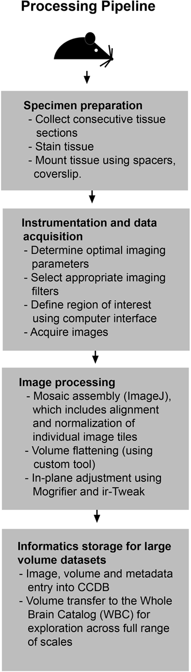
Figure 1. Processing pipeline flowchart. This flowchart illustrates the steps required to generate a 3D reconstruction of serial large-scale brain mosaics starting with specimen preparation and ending with deposition of datasets into publicly available databases.

Materials and Methods

Subjects

For this experiment, we used three male Balb C mice (Harlan Labs) each approximately 2 months old. Mice were housed in an animal care facility on a 12-h light/dark cycle with food and water ad libitum. Animal care was in accordance with the Guide for Care and Use of Laboratory Animals (NIH publication 865-23, Bethesda, MD, USA) and approved by the Institutional Animal Care and Use Committee (IACUC).

Tissue Preparation

Animals were administered an intraperitoneal injection of pentobarbital (75 mg/kg) and subsequently perfused transcardially with 1×PBS (∼30 s). They were then perfused with a DiI (0.1 mg/mL) solution for 5 min followed by 0.1 M PBS containing 4% paraformaldehyde for 10 min (Li et al., 2008). Following brain removal, the whole brain was postfixed overnight in 4% paraformaldehyde at 4°C. This overnight fixation step ensures better quality of vibratomed sections and reduces the number of tears in the final sections.

Tissue Processing

Following overnight postfixation, the brain was cut into two hemispheres and sectioned serially into 50-μm-thick slices using a vibratome, sagittally for the left hemisphere and coronally for the right hemisphere. All sections were stored in cryoprotectant at −20°C before staining tissue.

Next, free-floating sections were washed three times with 1×PBS for 5 min. Sections were then stained with FluoroMyelin Green (1:100; Invitrogen) overnight at 4°C on a rocker. The following day, sections were washed three times with 1×PBS for 5 min and then stained with TO-PRO-3 (1:3000; Invitrogen) for 45 min at room temperature. Sections were washed three times with 1×PBS for 5 min before mounting on glass slides with Gelvatol (Harlow and Lane, 1988).

Finally, special measures were taken to ensure careful mounting of tissue sections with as little distortion as possible during cover-slipping. To minimize compression by the glass coverslip, spacers of a thickness of 75 μm were used.

Instrumentation and Data Acquisition

A FluoView 1000 (Olympus Center Valley, PA, USA) equipped with a 40× NA 1.3 oil immersion objective and a high-precision motorized stage was used to collect the large-scale 3D mosaics of each tissue section. The boundaries (in x, y, and z) of the tissue section were defined using the Multi-Area Time Lapse function of ASW 1.7c microscope operating-software provided by Olympus (Olympus, Center Valley, PA, USA). The software automatically generates a list of 3D stage positions covering the volume of interest, which are computed using the dimensions of a single image in microns, degree of overlap between adjacent images and z-step size. Individual image tiles were 512 × 512 with a pixel dimension of 0.62 μm; overlap between two adjacent images (x–y) was 10% and the z-step was 5 μm; there is no overlap in z. The specimen was excited sequentially with a laser at three different wavelengths: 561, 488, 633 nm, which respectively excites the DiI, the FluoroMyelin, and the TO-PRO-3. For each of the channels, the output signal was filtered using a band-pass emission filter (between 500 and 550 nm for the DiI, 570 and 625 nm for the FluoroMyelin) or a high-pass emission filter (cut off at 650 nm for TO-PRO-3). The final data is stored in a RGB image volume, where the color channels map the specimen susceptibility at wavelengths 561, 488, 633 nm (corresponding to DiI, FluoroMyelin, and TO-PRO-3, respectively). Unprocessed data was stored as a single image stack containing information about the relative position of each image tile. No deconvolution was necessary.

Image Processing

In order to generate the final reconstructed 3D volume, several image processing steps are required, which include: mosaic assembly of each section volume, volume flattening of each section, and in-plane adjustment for stacking sequential section volumes. Each of these steps is necessary because of the challenges that accompany the process of stacking individual serial tissue sections. Not only the initial orientation of each section is different, but also the tissue can undergo severe stress or damage at either the sectioning or the cover-slipping stages as mentioned above. The resulting distortions need to be corrected before the stacking process can begin. These three steps are described in detail in the following paragraphs.

The mosaic assembly process is well documented in the case of a single tissue section and can be performed using an available ImageJ plug-in, ME Montage (Chow et al., 2006; Price et al., 2006). Images are first normalized so that all image tiles match each other in contrast and intensity for a seamless reconstruction of the final montage. Next, each volume is digitally flattened along the same orientation using a procedure developed at NCMIR and available online¹. Finally, large-scale mosaics are opened in Mogrifier or ir-Tweak so that sections can be registered using points/landmarks in the tissue such as large blood vessels and myelin.

Mosaic assembly

Mosaics are assembled using a set of plug-ins for ImageJ². The plug-in package is called ME Montage and is available online³.

Alignment and normalization of the image tiles have been previously described in detail for single sections (Chow et al., 2006). Briefly, the first step is a preprocessing step that separates images into individual channels. Next, each channel is normalized. Uneven illumination is evaluated heuristically from the entire set of acquired data for each channel and then corrected systematically in each image tile. This is followed by an automatic alignment and combining step, which aligns and stitches all of the image tiles of a given z-step within the same channel.

In this study, the number of image tiles required for each section was approximately 20 × 25 × 15 = 7,500 tiles for a single hemi coronal tissue section and 55 × 25 × 15 = 20,625 tiles for a sagittal section.

Volume flattening

Volume flattening was implemented as described below using a software package available online. The process consists of local expansion and compression applied along the z axis, which is roughly perpendicular to the sections.

As a preliminary step to the flattening, the top, and bottom surfaces of the sections must be delineated, see Figure 2A. This operation is done with the IMOD software (Kremer et al., 1996), a viewer tool specifically developed for dealing with 3D images in the MRC format; IMOD is widely used in the electron tomography community, allowing one to use volume density as a template to create 3D model structures made of objects, contours, and points. Typically in our case, two objects are created, one for each boundary of the specimen, see Figure 2B; points belonging to the surfaces are then manually picked on a roughly regular x–y grid, and added to their corresponding object.

FIGURE 2

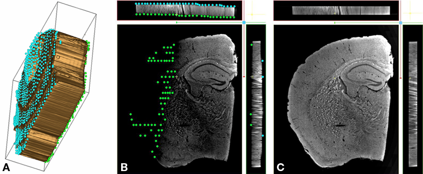
Figure 2. Volume flattening process. (A) Isosurface of a single mouse brain coronal section. The two boundary surfaces are delimited by two sets of points (in green and in blue). This 3D plot clearly shows the section unevenness that is corrected for during the flattening step. (B) XYZ view of a warped mouse brain coronal section within the IMOD viewer. The volume density has been converted from RGB to gray scale. Two objects consisting of a set of points (respectively in green and in blue) model the spatial variation of the section boundaries. These points are used as references during the flattening procedure. The specimen aspect ratio was modified and stretched along the z direction to allow the manual positioning of the marker points in the viewer. (C) XYZ view of a flattened mouse brain coronal section within the IMOD viewer. A warped section is submitted to local compressions/expansions along z the direction, forcing the specimen boundaries onto two parallel planes. The transformation leaves the section volume unchanged.

Thickness of the tissue sections in our light microscopy study averages 50 μm, while the overall field of view is relatively large (ranging to more than half a centimeter for the whole mosaic). With a z-step size of 5 μm, the number of acquired slices for a single tissue section ends up extremely small relative to the number of pixels in x–y, making it difficult to position tracking points within the displayed transverse view. To bypass this problem, the initial volume is first stretched in the z direction; this allows working from three simultaneous views (front, top, and side) in IMOD, see Figure 2C. Note that a gray scale version of the volumes is used to track the section boundaries; currently IMOD does not allow multiple views for RGB images.

In this model, section boundaries are described by two surfaces defined as z = f₁(x, y) and z = f₂(x, y), where f₁ and f₂ are taken as polynomial functions; the volume density, denoted u(x, y, z), is composed of the three color channels u(x, y, z) = [u_c(x, y, z)]_{c ∈RGB}. The two functions f₁ and f₂ are evaluated by regression to fit the marker data points previously outlined in IMOD. The polynomial order chosen for f₁ and f₂ depends on the number of markers and their distribution; the higher the marker density, the higher the order. The marker distribution does not need to be strictly regular; fewer points are needed on the slowly varying part of the surface, but as a rule there should not be any empty region (in x and y) free of “markers.” Note that outside of the reconstruction for z < f₁(x, y) and z > f₂(x, y), u_c(x, y, z) ≈ 0 for each color channel.

To flatten the volume, an appropriate transformation that associates u = [u_c]_c∈RGB to the volume density of a flat section delimited by two plane boundaries z = z₁ and z = z₂ is required. In our solution, we use a shear type de-warping procedure. It consists of readjusting the volume density along the z direction to be delimited by [z₁, z₂]. The flattened density u_c for each channel is then:

where is given by:

Finally, an additional constraint between z₁ and z₂ needs to be assumed. The transformation is isovolumic with the same overall volume for the warped and flattened section. Other alternatives consist of setting the difference z₂ − z₁ to match either the minimal, average, or maximal width of the original warped volume.

This flattening method is strictly a 1D problem, and thus easy to implement. In Figure 3, we show how the flattening procedure transforms an uneven section into a flat one.

FIGURE 3

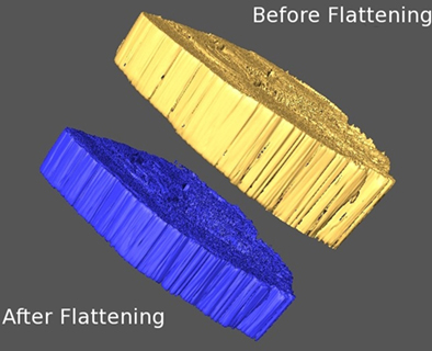
Figure 3. Before and after flattening. Isosurfaces are plotted for an uncorrected digital section (yellow) and its corrected volume after the flattening (blue).

In-plane adjustment

Once sections are flattened, it is possible to pile them into a z-sequence; however, further adjustments in the x–y direction remain necessary to obtain flawless stitching. Our approach consists of warping a whole section in x–y (independently of z) resulting in a first optical slice that matches the last optical slice of the previous section, see Figure 4.

FIGURE 4

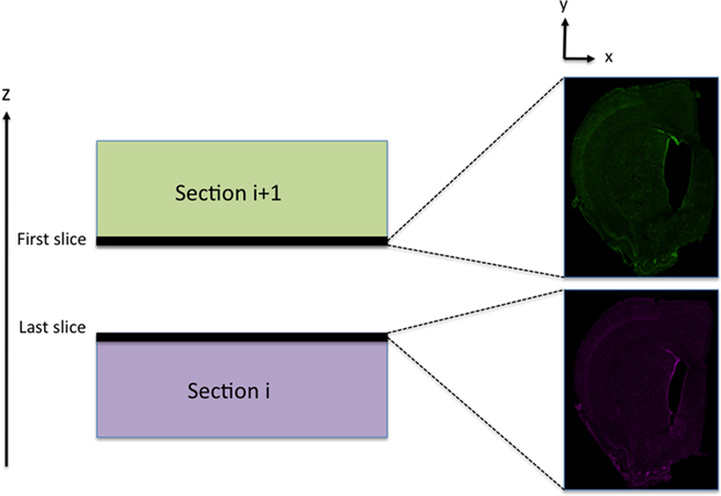
Figure 4. Aligning adjacent sections. Slices used to register two adjacent sections during the in-plane adjustment. The first slice of a section (i + 1) should match the last slice of the previous section (i).

Two interactive tools allowing registration between 2D images are freely available: Mogrifier⁴ and ir-Tweak⁵ (Anderson et al., 2009). We used these tools to calculate and implement the warping transformation allowing a smooth transition from one section to the next. Alignment and warping, for both tools, is accomplished by setting linked correspondences between the reference image and the image to be warped. These correspondence points are used as reference points, and a thin plate spline (Belongie, 2010) is used to evaluate the full image transformation.

While similar in nature, Mogrifier and ir-Tweak have a few notable differences. Mogrifier is a Java Web Start application that can operate on arbitrarily large images by decomposing the image into tiles at several levels of detail, allowing the user to dynamically zoom into detail or zoom out for an overall synoptic view. The user interactively marks up the image with reference points, see Figure 5, and can perform test warpings until the appropriate degree of fit is accomplished. Warping on the full sized image is then performed using the same algorithm on a 32 node computational cluster.

FIGURE 5

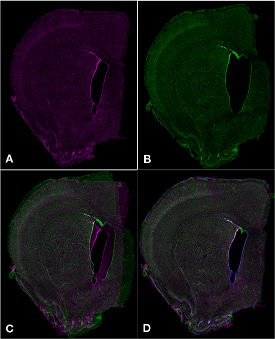
Figure 5. Aligning serial sections using Mogrifier. Two serial coronal sections (A,B) are shown as they would appear in Mogrifier (i.e., in red and green channels). Image (B) illustrates an example of non-uniform compression of the lateral ventricle in a tissue section. Image (C) shows the overlay of slices (A,B) in the application Mogrifier before applying any transformation. Image (D) shows the overlay of slices (A,B) and the reference points (blue) after applying the thin plate spline transformation in Mogrifier.

Ir-Tweak is an interactive, multi-threaded, and cross-platform application as well. It implements fragment shading in order to reduce the memory footprint of the image textures. Its level of interactivity is slightly more sophisticated than Mogrifier in that the transform parameters and warped image are automatically updated as control points are placed in the images, see Figure 6.

FIGURE 6

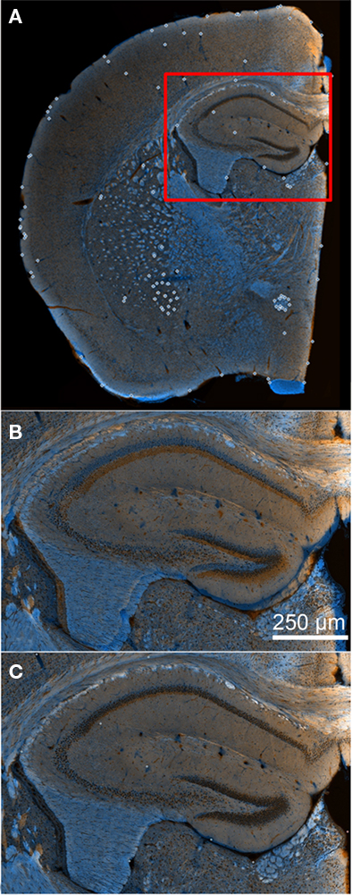
Figure 6. Aligning serial sections using ir-Tweak. Image (A) shows a wide-field view of overlaid adjacent slices in the application ir-Tweak (reference points shown as white open circles) before applying any transformation. Image (B) shows a high-magnification image of the hippocampus from (A). This image demonstrates the mis-alignment of serial sections before applying the thin plate spline transformation in ir-Tweak. Image (C) shows the same high-magnification image from (B) after applying the thin plate spline transformation in ir-Tweak.

We found Mogrifier to be a very effective tool when the x–y tissue distortions are large (see Figure 5 for an example of large tissue distortion); on the contrary, the ir-Tweak software is a better solution for implementing small adjustments between two adjacent sections.

Each time a new section is added on the stack, all its z-slices are uniformly transformed within the x–y plane following the Mogrifier/ir-Tweak warping correction.

In our brain study, landmarks such as myelin, blood vessels, cell layers, ventricles, and edges of tissue section provide reliable reference points for warping. Individual cells stained with a nuclear label (TO-PRO-3) cannot be used reliably as reference points; however, they can be used to identify key brain regions/cell layers, which can then be used as reference points. In Figure 6, examples of reliable reference points are shown in pictures before and after applying the warping transformation in ir-Tweak.

For the final reconstructed volume presented in this paper, see Figure 7; Movies S1 and S2 in Supplementary Material, the warped sections were first coarsely adjusted with Mogrifier; subsequently, they were flattened, and finally a fine-tune adjustment in the stitching was implemented with ir-Tweak. The first and third steps are slightly redundant, and in a regular flow only two steps, (1) a flattening followed by (2) an in-plane adjustment, should be sufficient after the mosaic assembly is completed. Movies of the final volume were generated using Imaris (Bitplane Inc., St. Paul, MN, USA) and Amira (Visage Imaging, Inc., San Diego, CA, USA).

FIGURE 7

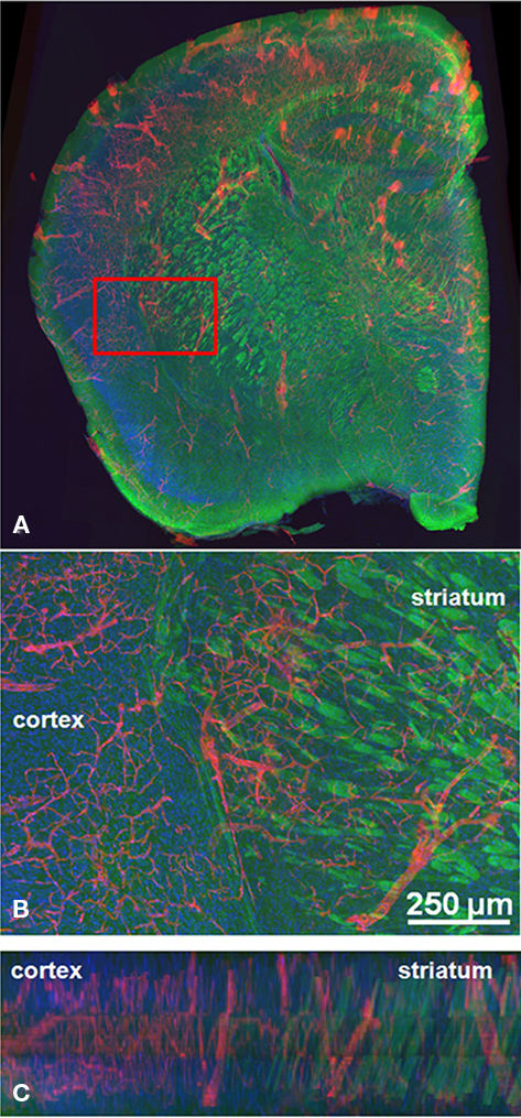
Figure 7. Volume reconstruction evaluation. (A) A series of three coronal sections was successfully labeled with fluorescent stains, imaged, flattened, and reconstructed using Mogrifier and ir-Tweak. A higher magnification image is shown (B) where the three labels (DiI in red for the blood vessels, FluoroMyelin in green for the myelin, and TO-PRO-3 in blue for the nuclei) are more clearly discernible in the striatum and the cortex. A cross-section (x–z plane) of this same sample region is shown in (C). The alignment of the blood vessels (DiI) and FluoroMyelin can be seen more easily in this cross-section. These images were collected in Imaris, an application for 3D visualization and segmentation.

Informatics Resources for Large Volume Datasets

The underlying long-term goal of this study is to build a digital 3D reconstruction of a brain populated with reconstructions of individual cells acquired with high-resolution LM or EM techniques. With a pixel dimension of 0.62 μm in x and y and an overall scale of a few millimeters (5 mm × 5 mm for a coronal hemisection), the number of pixels per mosaic slice in z can reach 5 × 10⁷. The length of the brain along the rostral–caudal axis is ∼1 cm, corresponding to approximately 200 vibratomed 50-μm-thick coronal sections. A digital RGB reconstruction for the whole brain would then correspond approximately to 80 GB of raw data.

For this study, we used a desktop computer with 16 GB of RAM, dual core Intel Xeon 5160 3 GHz ×2 processor. The graphical card was a NVidia Quadro FX 4500. For visualization, we used a binned version of the final volume; this down-sampled dataset is easier to manipulate from a graphical interface. In this preliminary study, we did a partial reconstruction using three serial coronal hemisections. A snapshot of this reconstruction can be seen in Figure 7. Even in this case, the sample volume requires several gigabytes of memory storage. The mosaic stitching was automatically done overnight, while the flattening/stacking of the final sections required a few hours of computational processing. However, the manual step of selecting the reference points (both for the flattening and warping steps) remained the most time-consuming operation and the bottle-neck of the whole process. Further studies should focus on automating this step.

In order to work with such large volumes of data, a specific environment is needed for extracting quantitative information. Two valuable database resources providing a shared, online atlasing environment to the neuroscience community are the cell centered database (CCDB) and the Whole Brain Catalog (WBC). CCDB offers biologists a platform to store and publish their large datasets, making them available to other scientists. Additionally, our data is also available on WBC. The WBC allows multi-scale data from the brain to be represented in a common space accessible to neuroscientists across disciplines. It is an interactive viewing environment drawing from multiple data repositories across the world. All of the data for this project can be found at http://ccdb.ucsd.edu by searching under the project ID# P2023.

Results and Discussion

Automated image acquisition of large-scale brain mosaics in light microscopy is contributing to an increasing pace of scientific discovery. Wide-field views of whole brain tissue sections with sub-micron pixel resolution provide the researcher with a detailed panorama of specimens and vast amounts of data analysis. In conjunction with image databases and neuroinformatics tools, these datasets can be shared, annotated, and enriched by researchers worldwide. Data are already coming from many places such as the Allen Brain Atlas (ABA; Lein et al., 2007), Neuroscience Information Framework (NIF; Gardner et al., 2008), CCDB (Martone et al., 2003), and are streaming into shared multi-scale volume environments like the WBC⁶ – a critical framework onto which contributors may deposit, view, and interact with their light microscopic data in their tissue context.

In this paper, we have outlined the techniques needed to stitch a small portion of the whole mouse brain. These techniques deal with both specimen preparation and data processing steps. In this approach, the 3D digitized volumes of the tissue sections are geometrically re-touched in order to generate a final continuous volume. All the sections are flattened and then registered to one another using software tools already developed and freely available.

Previously described techniques for volume reconstruction from serial sections are typically limited to small regions within the brain (Lee and Bajcsy, 2008). A more recent paper (Capek et al., 2009) describes a similar method for dealing with volume reconstruction of large specimens, but does not address the problem of out-of-plane distortions, which was an issue we needed to address in our large-scale volume reconstruction. Such variations in distortion could be the result of differences in specimen preparation methods between the two papers; however, our procedures for sectioning and staining are standard methods used for confocal microscopy, thus emphasizing the utility of the volume reconstruction steps outlined in this methods paper. The volume reconstruction technique described here builds on these previous tools by allowing researchers to image whole brain sections using tissue sections labeled with fluorescent dyes and imaged on a confocal microscope. Depending on the staining or immunolabeling method used, one must choose a section thickness in accordance with the depth of penetration of the fluorescent label and the imaging limitations of the light microscope used.

An evaluation method for this technique is limited by the imaging range of the confocal microscope. For example, one way to evaluate the quality of our 3D reconstruction is to compare the final reconstructed volume of three serial tissue sections (of 50 μm thickness) to a fully imaged intact tissue section of 150 μm thickness. Standard confocal microscopy cannot image through such a thick section, thus we attempted to image one of these hemisections on a two photon microscope. The FluoroMyelin label photobleached quickly and bleed-through between channels was also a problem. Since the two-photon microscope does not allow for sequential channel acquisition, an evaluation method of this nature was not possible. Instead, we have visually evaluated the 3D reconstructed volume using Imaris, which allows the user to rotate and inspect volumes in 3D. Some imperfections remain noticeable, for instance, the density mismatch between adjacent sections, as seen in Figure 7C (line artifacts perpendicular to z in the x–z top view). Normalizing the density between sections cannot completely correct these types of artifacts because of the inherent physical differences in imaging the top versus the bottom of a section.

With two recently developed image processing tools, ir-Tweak and Mogrifier, we are now able to stitch together several of these brain mosaic sections after digital flattening, resulting in a serial 3D reconstruction for a more global analysis of the brain. Both ir-Tweak and Mogrifier can handle large file sizes and repair some of the typical specimen preparation artifacts that have made 3D reconstructions of this nature difficult in the past.

Note that our procedure is not absolute, but is a reasonable and practical stitching solution when tissue distortions remain overall small. For example, in the case of a very strong warping for instance (or if the width variations in a tissue block are big), sections could be warped back close to their original shape (after processing and alignment) to limit any artificial geometrical distortion in the final reconstructed volume. A potential alternative to the multi-step flattening/stitching approach used here would be a tool capable of manipulating volumes in 3D.

This work is the first step toward creating a 3D reconstruction of the mouse brain using standard vibratome sections and large-scale mosaics. The next logical step is to apply this reconstruction technique to compare the brains of a wild type mouse and a mouse model for human neurological disorders. Applied to mouse models of neurological disorders, this technique should be helpful for studying wide-scale alterations in brain structures (e.g., changes in vasculature associated with disease or injury). Moreover, using a transgenic mouse with endogenous fluorescent proteins would simplify this process by eliminating the need for staining procedures, while at the same time pinpointing a specific biological target. Such future applications of the presently described technique could pave a novel way for scientists to study and share information about the brain’s neuronal circuitry.

Conflict of Interest Statement

The authors declare that the research was conducted in the absence of any commercial or financial relationships that could be construed as a potential conflict of interest.

Acknowledgments

This study was made possible by National Institutes of Health (NIH) grant numbers P41 RR004050 from the National Center for Research Resources (NCRR) and R01 EB005832 from the National Institute of Biomedical Imaging and Bioengineering, and the Waitt Family Foundation.

Supplementary Material

The Movies 1 and 2 for this article can be found online at http://www.frontiersin.org/neuroanatomy/10.3389/fnana.2011.00017/abstract

Movie S1. Final volume reconstruction. A movie clip traveling through an aligned stack of three hemi coronal sections reconstructed using the specimen preparation and software steps outlined in this methods paper.

Movie S2. XYZ view of final reconstruction. A movie of the XYZ view of the final reconstructed volume in Amira. This animation demonstrates the precision of the alignment of labeled landmarks within the final volume.

Footnotes

1. ^https://confluence.crbs.ucsd.edu/pages/viewpage.action?pageId=13042141
2. ^http://rsb.info.nih.gov/ij
3. ^https://confluence.crbs.ucsd.edu/display/ncmir/Mosaic+Plug-ins+for+ImageJ
4. ^http://ncmir.ucsd.edu/downloads/mogrifier/mogrifier.shtm
5. ^http://www.sci.utah.edu/download/ncrtoolset/1.0.html
6. ^http://wholebraincatalog.org/

References

Ai, Z., Chen, X., Rasmussen, M., and Folberg, R. (2005). Reconstruction and exploration of three-dimensional confocal microscopy data in an immersive virtual environment. Comput. Med. Imaging Graph. 29, 313–318.

Pubmed Abstract | Pubmed Full Text | CrossRef Full Text

Anderson, J. R., Jones, B. W., Yang, J. H., Shaw, M. V., Watt, C. B., Koshevoy, P., Spaltenstein, J., Jurrus, E., Kannan, U. V., Whitaker, R. T., Mastronarde, D., Tasdizen, T., and Marc, R. E. (2009). A computational framework for ultrastructural mapping of neural circuitry. PLoS Biol. 7, e1000074. doi: 10.1371/journal.pbio.1000074

Pubmed Abstract | Pubmed Full Text | CrossRef Full Text

Belongie, S. (2010). “Thin plate spline,” in From MathWorld – A Wolfram Web Resource, ed. E. W. Weisstein. Available at: http://mathworld.wolfram.com/ThinPlateSpline.html

Braumann, U. D., Scherf, N., Einenkel, J., Horn, L. C., Wentzensen, N., Loeffler, M., and Kuska, J. P. (2007). Large histological serial sections for computational tissue volume reconstruction. Methods Inf. Med. 46, 614–622.

Pubmed Abstract | Pubmed Full Text

Capek, M., Bruza, P., Janacek, J., Karen, P., Kubinova, L., and Vagnerova, R. (2009). Volume reconstruction of large tissue specimens from serial physical sections using confocal microscopy and correction of cutting deformations by elastic registration. Microsc. Res. Tech. 72, 110–119.

Pubmed Abstract | Pubmed Full Text

Chow, S. K., Hakozaki, H., Price, D. L., MacLean, N. A., Deerinck, T. J., Bouwer, J. C., Martone, M. E., Peltier, S. T., and Ellisman, M. H. (2006). Automated microscopy system for mosaic acquisition and processing. J. Microsc. 222, 76–84.

Pubmed Abstract | Pubmed Full Text | CrossRef Full Text

Gardner, D., Akil, H., Ascoli, G. A., Bowden, D. M., Bug, W., Donohue, D. E., Goldberg, D. H., Grafstein, B., Grethe, J. S., Gupta, A., Halavi, M., Kennedy, D. N., Marenco, L., Martone, M. E., Miller, P. L., Muller, H. M., Robert, A., Shepherd, G. M., Sternberg, P. W., Van Essen, D. C., and Williams, R. W. (2008). The neuroscience information framework: a data and knowledge environment for neuroscience. Neuroinformatics 6, 149–160.

Pubmed Abstract | Pubmed Full Text | CrossRef Full Text

Harlow, E., and Lane, D. (1988). Antibodies: A Laboratory Manual. Cold Spring Harbor, NY: Cold Spring Harbor Laboratory Press.

Ju, T., Warren, J., Carson, J., Bello, M., Kakadiaris, I., Chiu, W., Thaller, C., and Eichele, G. (2006). 3D volume reconstruction of a mouse brain from histological sections using warp filtering. J. Neurosci. Methods 156, 84–100.

Pubmed Abstract | Pubmed Full Text

Kremer, J. R., Mastronarde, D. N., and McIntosh, J. R. (1996). Computer visualization of three-dimensional image data using IMOD. J. Struct. Biol. 116, 71–76.

Pubmed Abstract | Pubmed Full Text

Lee, S. C., and Bajcsy, P. (2008). Trajectory fusion for three-dimensional volume reconstruction. Comput. Vis. Image Underst. 110, 19–31.

Pubmed Abstract | Pubmed Full Text | CrossRef Full Text

Lein, E. S., Hawrylycz, M. J., Ao, N., Ayres, M., Bensinger, A., Bernard, A., Boe, A. F., Boguski, M. S., Brockway, K. S., Byrnes, E. J., Chen, L., Chen, T. M., Chin, M. C., Chong, J., Crook, B. E., Czaplinska, A., Dang, C. N., Datta, S., Dee, N. R., Desaki, A. L., Desta, T., Diep, E., Dolbeare, T. A., Donelan, M. J., Dong, H. W., Dougherty, J. G., Duncan, B. J., Ebbert, A. J., Eichele, G., Estin, L. K., Faber, C., Facer, B. A., Fields, R., Fischer, S. R., Fliss, T. P., Frensley, C., Gates, S. N., Glattfelder, K. J., Halverson, K. R., Hart, M. R., Hohmann, J. G., Howell, M. P., Jeung, D. P., Johnson, R. A., Karr, P. T., Kawal, R., Kidney, J. M., Knapik, R. H., Kuan, C. L., Lake, J. H., Laramee, A. R., Larsen, K. D., Lau, C., Lemon, T. A., Liang, A. J., Liu, Y., Luong, L. T., Michaels, J., Morgan, J. J., Morgan, R. J., Mortrud, M. T., Mosqueda, N. F., Ng, L. L., Ng, R., Orta, G. J., Overly, C. C., Pak, T. H., Parry, S. E., Pathak, S. D., Pearson, O. C., Puchalski, R. B., Riley, Z. L., Rockett, H. R., Rowland, S. A., Royall, J. J., Ruiz, M. J., Sarno, N. R., Schaffnit, K., Shapovalova, N. V., Sivisay, T., Slaughterbeck, C. R., Smith, S. C., Smith, K. A., Smith, B. I., Sodt, A. J., Stewart, N. N., Stumpf, K. R., Sunkin, S. M., Sutram, M., Tam, A., Teemer, C. D., Thaller, C., Thompson, C. L., Varnam, L. R., Visel, A., Whitlock, R. M., Wohnoutka, P. E., Wolkey, C. K., Wong, V. Y., Wood, M., Yaylaoglu, M. B., Young, R. C., Youngstrom, B. L., Yuan, X. F., Zhang, B., Zwingman, T. A., and Jones, A. R. (2007). Genome-wide atlas of gene expression in the adult mouse brain. Nature 445, 168–176.

Pubmed Abstract | Pubmed Full Text | CrossRef Full Text

Li, Y., Song, Y., Zhao, L., Gaidosh, G., Laties, A. M., and Wen, R. (2008). Direct labeling and visualization of blood vessels with lipophilic carbocyanine dye DiI. Nat. Protoc. 3, 1703–1708.

Pubmed Abstract | Pubmed Full Text | CrossRef Full Text

Martone, M. E., Zhang, S., Gupta, A., Qian, X., He, H., Price, D. L., Wong, M., Santini, S., and Ellisman, M. H. (2003). The cell-centered database: a database for multiscale structural and protein localization data from light and electron microscopy. Neuroinformatics 1, 379–395.

Pubmed Abstract | Pubmed Full Text | CrossRef Full Text

Price, D. L., Chow, S. K., Maclean, N. A., Hakozaki, H., Peltier, S., Martone, M. E., and Ellisman, M. H. (2006). High-resolution large-scale mosaic imaging using multiphoton microscopy to characterize transgenic mouse models of human neurological disorders. Neuroinformatics 4, 65–80.

Pubmed Abstract | Pubmed Full Text | CrossRef Full Text

Tasdizen, T., Koshevoy, P., Grimm, B. C., Anderson, J. R., Jones, B. W., Watt, C. B., Whitaker, R. T., and Marc, R. E. (2010). Automatic mosaicking and volume assembly for high-throughput serial-section transmission electron microscopy. J. Neurosci. Methods 193, 132–144.

Pubmed Abstract | Pubmed Full Text