Multiscale exploration of mouse brain microstructures using the knife-edge scanning microscope brain atlas
- 1 Samsung Electronics, Suwon, Republic of Korea
- 2 Department of Computer Science and Engineering, Texas A&M University, College Station, TX, USA
- 3 Beckman Institute of Advanced Science and Technology, University of Illinois, Urbana-Champaign, IL, USA
- 4 Department of Electrical and Computer Engineering, Kettering University, Flint, MI, USA
- 5 Research and Development, 3Scan, Bryan, TX, USA
- 6 Department of Veterinary Integrative Biosciences, Texas A&M University, College Station, TX, USA
Connectomics is the study of the full connection matrix of the brain. Recent advances in high-throughput, high-resolution 3D microscopy methods have enabled the imaging of whole small animal brains at a sub-micrometer resolution, potentially opening the road to full-blown connectomics research. One of the first such instruments to achieve whole-brain-scale imaging at sub-micrometer resolution is the Knife-Edge Scanning Microscope (KESM). KESM whole-brain data sets now include Golgi (neuronal circuits), Nissl (soma distribution), and India ink (vascular networks). KESM data can contribute greatly to connectomics research, since they fill the gap between lower resolution, large volume imaging methods (such as diffusion MRI) and higher resolution, small volume methods (e.g., serial sectioning electron microscopy). Furthermore, KESM data are by their nature multiscale, ranging from the subcellular to the whole organ scale. Due to this, visualization alone is a huge challenge, before we even start worrying about quantitative connectivity analysis. To solve this issue, we developed a web-based neuroinformatics framework for efficient visualization and analysis of the multiscale KESM data sets. In this paper, we will first provide an overview of KESM, then discuss in detail the KESM data sets and the web-based neuroinformatics framework, which is called the KESM brain atlas (KESMBA). Finally, we will discuss the relevance of the KESMBA to connectomics research, and identify challenges and future directions.
1 Introduction
Connectomics aims to map the full connection matrix of the brain (Sporns et al., 2005; Sporns, 2011). The fundamental assumption in connectomics is that structure defines function. To evaluate this assumption, we can consider the fact that the functional evolution of the brain has been mainly driven by that of the brain architecture and not by individual neurons (Swanson, 2003). Also, “basic circuits” of the brain have been identified as an important abstraction of brain function at the system-level (Shepherd, 2003). Furthermore, structure (connectivity) has been shown to greatly affect the dynamics of the network (Sporns and Tononi, 2002). Varying the delay distribution in a network was also found to alter its dynamics (Thiel et al., 2003), where structural analogs of delay, e.g., connection length, could also contribute to the same effect. These, taken together, indicate that obtaining the connectome can lead to a major breakthrough in understanding brain function.
Recent advances in high-throughput, high-resolution 3D microscopy methods have enabled the imaging of whole small animal brains at a sub-micrometer resolution, potentially opening the road to full-blown connectomics research. One of the first such instruments to achieve whole-brain-scale imaging at sub-micrometer resolution is the Knife-Edge Scanning Microscope (KESM; McCormick, 2003, 2004; Kwon et al., 2008; Mayerich et al., 2008b; cf. Li et al., 2010 based on the same imaging principles as that of the KESM). KESM whole-brain data sets now include Golgi (neuronal circuits; Abbott, 2008), Nissl (soma distribution; Choe et al., 2010), and India ink (vascular networks; Choe et al., 2009; Mayerich et al., 2011b). Methods related to the KESM include All-Optical Histology (Tsai et al., 2003) and Array Tomography (Micheva and Smith, 2007). There are also methods that explore much finer structural detail, such as Serial Block-Face Scanning Electron Microscopy (SBF-SEM; Denk and Horstmann, 2004), and Automatic Tape-Collecting Lathe Ultramicrotome (ATLUM; Hayworth, 2008). The resolution and size of the volume that can be imaged by the above methods vary widely (resolution of 10s of nm to 100s of nm, to volumes ranging from 10s of μm cube up to 1 cm cube; see Choe et al., 2008 for a review), but they all share the same principle of physical sectioning or physical ablation, as opposed to optical sectioning common in conventional 3D microscopy (All-Optical Histology uses a hybrid approach, physical plus optical sectioning; Tsai et al., 2003).
Data from KESM and similar approaches based on light microscopy can greatly contribute to connectomics research, by filling the critical gap between large scale, lower resolution methods like diffusion MRI (Basser and Jones, 2002; Tuch et al., 2003; Hagmann et al., 2007; Roebroeck et al., 2008) on the one hand and small-scale, higher resolution methods like SBF-SEM (Denk and Horstmann, 2004) on the other hand. It is also notable that KESM data are by nature multiscale, ranging from the subcellular (<1 μm) to the whole organ scale (∼1 cm). Due to the large volume (several tera voxels) and the multiscale nature, visualization alone is a huge challenge, before we even start worrying about quantitative connectivity analysis. Furthermore, delivering the neuronal circuit data to connectomics researchers is also a challenge, due to the same reasons as above. To solve this issue, we developed a web-based neuroinformatics platform for efficient visualization and analysis of the multiscale KESM data sets.
In this paper, we will first provide an overview of KESM, then discuss in detail the web-based neuroinformatics framework called the KESM brain atlas (KESMBA). Next, we will present the KESM data sets using KESMBA. Finally, we will discuss the relevance of the KESMBA to connectomics research, and identify challenges and future directions.
2. Materials and Methods
2.1. Specimen Preparation
Two mouse brains were imaged in their entirety, after being stained by Golgi-Cox for the visualization of neuronal morphology. C57BL/6J mice were anesthetized with isoflurane inhalant anesthesia. Each mouse was decapitated, the brain removed and immersed in Golgi-Cox solution that contained 1% potassium chromate, 1% potassium dichromate, and 1% mercuric chloride in distilled water. The brain was then soaked for 10–16 weeks in the dark and then washed in distilled water overnight. Additionally, it was immersed in a 5% ammonium hydroxide solution in distilled water for about one week in the dark and then again washed in distilled water for 4 h. After that, the brain was dehydrated through a graded series of ethanols starting with 50% ethanol in water and increasing to 100% ethanol over a time period of 6 weeks. Finally, it was embedded in araldite following a standard protocol (Abbott and Sotelo, 2000), with the exception that each step needed to infiltrate the brains with araldite took 24 h. KESM sectioning requires that whole-brains be completely dehydrated and infiltrated with araldite plastic. Normal plastic embedding is typically carried out on much smaller pieces of tissue, so we have modified the processing steps to allow us to embed whole mouse brains that we can cut using the KESM.
2.2. Imaging with the Knife-Edge Scanning Microscope
We used the KESM for sectioning and imaging (Mayerich et al., 2008b) two prepared mouse brains (both Golgi). Figure 1 shows a photo of the KESM with its major components.
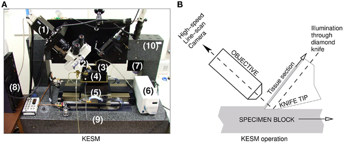
Figure 1. The knife-edge scanning microscope and its operation. (A) The Knife-Edge Scanning Microscope and its main components are shown: (1) high-speed line-scan camera, (2) microscope objective, (3) diamond knife assembly and light collimator, (4) specimen tank (for water immersion imaging), (5) three-axis precision air-bearing stage, (6) white-light microscope illuminator, (7) water pump (in the back) for the removal of sectioned tissue, (8) PC server for stage control and image acquisition, (9) granite base, and (10) granite bridge. (B) The imaging principle of the KESM is shown.
Each stained mouse brain, embedded in a plastic block, was mounted on the three-axis precision stage. The diamond knife-collimator assembly was used to cut sequential 1.0 μm-thick sections from the tissue blocks, while providing transmission illumination. (Note that the KESM design supports illumination through the objective (McCormick, 2004) and the original implementation already includes this design, especially for fluorescence imaging.) The light passed through the diamond knife and penetrated the tissue sections for imaging. The brain tissues stained in Golgi were imaged with a Nikon Fluor 10× objective (NA = 0.3). The actual image digitizing was performed by a DALSA CT-F3 high-sensitivity line-scan camera capturing the transmitted light, and these images were stored in the designated storage. In order to automatically control the stage movement and data acquisition process, we developed in-house control software (Kwon et al., 2008). Noise due to the knife-edge misalignment, defects in the knife blade, and knife chatter were removed through image processing algorithms including light normalization (Mayerich et al., 2007). The KESM controller also employed a stair-step cutting algorithm to minimize damage to tissue between neighboring columns (Kwon et al., 2008). After preliminary image processing for noise and distortion removal, TIFF formatted raw image files were compressed into high quality JPEG format and stored for further processing, while the original TIFF images were kept for archival purposes. We imaged horizontal sections from the brain.
2.3. The KESM Brain Atlas
The KESM brain atlas (KESMBA) framework has been designed and implemented to allow the widest dissemination of KESM mouse brain circuit data and to enable easy visual and quantitative analysis. For this, we had several design requirements, that the atlas is (1) not dependent on high-end computer hardware (e.g., expensive graphics cards), (2) not dependent on custom 3D viewing applications or plug-ins, and (3) browsable within any standard web browser.
2.3.1. Basic idea: Transparent overlay with distance attenuation
The basic idea we use to meet the requirements listed above is transparent overlay of images with distance attenuation (Eng and Choe, 2008). Figure 2 shows the concept. Overlaying an image stack containing two intertwining objects (Figure 2A) to get minimum intensity projection (Figure 2B) results in the loss of 3D information. Interleaving each image with semi-opaque blank images brings out the 3D information (Figure 2C). This is similar to the artistic use of haze to achieve depth effect in a 2D medium (cf. Kersten et al., 2006). In practice, raw images containing data already have semi-opaqueness in the background once made transparent, so simply overlaying them results in the same kind of effect. This simple approach, when combined with a Google Maps™-like zoomable web interface, results in a powerful browsing environment for large 3D brain data. In fact, we customized and extended the Google Maps API (version 2) to construct the KSEMBA.
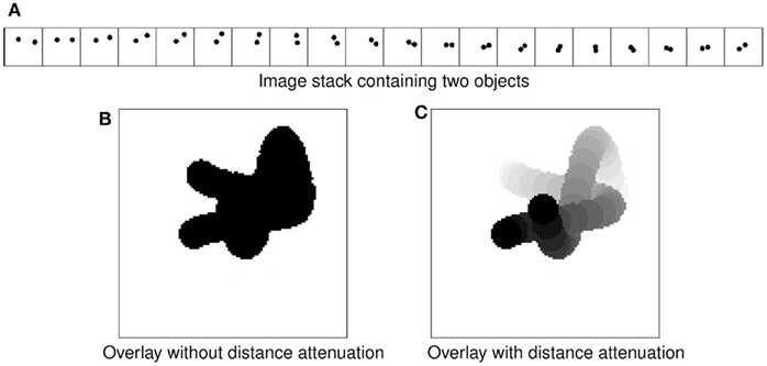
Figure 2. Transparent overlay with distance attenuation. (A) An image stack containing two intertwined objects are shown. (B) Simple overlay of the image stack in (A) results in loss of 3D perspective. (C) Overlay with distance attenuation helps bring out the 3D cue.
2.3.2. Image processing and adding transparency
After the raw image files were acquired using the KESM, three additional image processing steps were performed to enhance the image quality suitable for the web atlas. First, to enhance visibility when overlayed, we inverted the original images with black foreground and white background to have white foreground and black background. Next, because the inverted images do not have enough luminance contrast, we performed Gamma correction with a sigmoidal non-linearity to expand the luminance contrast between foreground and background pixels within each image. Finally, we turned the background color of the image to be transparent, for layering of the images to achieve a 3D view within a web browser. The pixels were made transparent according to their gray-level value. The processed images were stored in PNG format which supports alpha channel transparency. The contrast factor and contrast center values (25 and 50, respectively) used in the gray-level transparency process were empirically selected.
2.3.3. Multiscale tile generation
Once the image processing is done, pyramidal tiles are generated. Each tile in Google Maps consists of 256 × 256 pixels. The pyramidal structure of the Google Maps tiles in different zoom levels is shown in Figure 3A. Our Golgi data sets have 8–10 columns, where each column consists of a tall stack of 2,400 × 12,000-pixel images. Below, we will consider the case with 8 columns. Calculation for the 10 column case can be done in a similar manner.
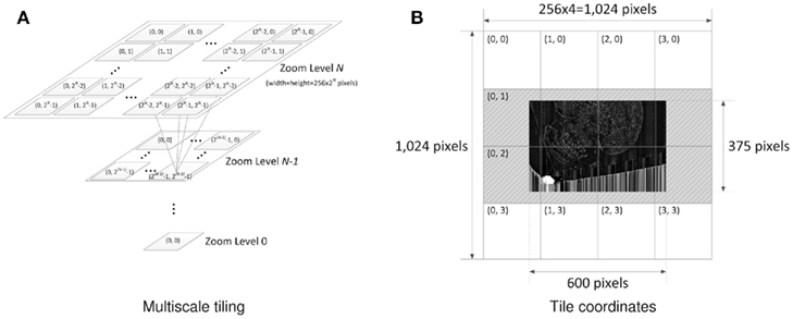
Figure 3. Multiscale tiling. (A) Tile pyramid compatible with GoogleMaps. Quad-tree pyramid of tiles and the x-y coordinate indexing convention are depicted. Each tile has 256 × 256 pixels. Zoom level ranges from 0 to 7, and zoom level N has 2N × 2N tiles. Following this tiling convention automatically enables various map functions including zoom-in/out. (B) Example of actual tiles. The maximum zoom level of the Golgi image section (19,200 × 12,000 pixels) is 7 [=argminx (256 × 2x ≥ max(19200,12000))]. The minimum zoom level is set to 2. This particular example shows how the original image is tiled and how the tiles are named at zoom level 2. The dark image in the middle is the image section halved down 5 times (600 × 375 pixels) to fit in zoom level 2 (1,024 × 1,024 pixels). After putting the downsized image at the center, transparent image patches (gray dashed area) are added to fill the incomplete tiles so that every tile can have the same 256 × 256 pixels size. Because there is no need to generate empty tiles, only 8 tiles are created out of 16 possible ones.
With the KESM image stack, we prepared tiles for 6 different zoom levels compatible with the Google Maps API’s zoom level from 2 to 7. The number of tiles required at zoom level z is 2z × 2z. Therefore, the Golgi data set requires  tiles for each section, and 121,692,480 tiles for all 5,572 sections, theoretically. Fortunately, the actual number of tiles we created is 4,892 per section and 27,258,224 overall because each image section is not square-shaped and we only had to create tiles containing tissue data. Figure 3B shows an example of the tiles we created for the highest zoom level of 7. In the example, we had to create only 8 tiles out of 16 possible ones because the other 8 tiles were empty. Preparing a tile pyramid requires extra storage, time, and effort. Assuming that the above mentioned PNG transform did not increase the file size, in our Golgi data set, the tile pyramid (4,892 × 256 × 256 × 5,572 = 320,002,112) causes about 39% increase in disk space usage (without tiles, the total size is 19,200 × 12,000 × 5,572 = 230,400,000). However, once they are generated, they contribute to saving image download time for the currently viewed portion of the atlas. For example, the KESMBA has a map area of 80% browser window width × 600 pixel window height specified in a Cascading Style Sheet (CSS). Given typical screen resolution, the number of 256 × 256 sized tiles concurrently displayed on a client web browser will be ∼30 at the maximum, which is less than 1% of the original image section at the maximum zoom level (19,200 × 12,000). Once all the tiles are generated, each tile is named consistent with Google Maps tile specification. For example, a tile name 1_2_3.png denotes zoom level = 1, x-coordinate = 2, and y-coordinate = 3.
2.3.4. Web atlas based on Google maps API
To enable 3D visualization, we customized the Google Maps JavaScript API. Google Maps JavaScript API provides extensive functions required for a geographical atlas. In addition to the essential navigational functions of zooming and panning, Google Maps JavaScript API offers useful features such as zoom scale bar, double-click zoom-in, and overlaying various objects including images, text, markers, and polygons. Google Maps provides an extensive API specification and there exist a large number of private developers seeking and sharing solutions for customizing the API.
2.3.4.1. Customizations. Existing API functions were customized to fit the purpose of the KESMBA. This customization included: using custom tiles; tile overlays; user options to select the number and interval of the tile overlays; overlaying zoomable annotation; and map redraw function. The API was further extended to include: information panel; scale bar; map capture button; and z-axis navigation controller.
We generated a custom map type instance of the “GMapType” class to call the map tiles from the Google database to feed in the custom tiles we generated. Multiple tiles from subsequent image sections are overlaid to create a 3D effect. The summary code below provides an overview of how this is achieved using the Google Maps API.
////////////////////

// File: overlay.js

////////////////////


…


// 1. Create a tile layer.

customLayer=[new GTileLayer(…)];


// 2. Generate a custom tile URL.

customLayer.getTileUrl=customGetTileUrl;


// 3. Create an overlay instance of

//      the GTileLayerOverlay class.

customOverlay=new GTileLayerOverlay

(customLayer);


// 4. Create a map type instance of the

//      GMapType class.

customMap=new GMapType(…);


// 5. Create a map instance of the GMap2

//      class.

var myMap=new GMap2(document.getElementById

("map"),

          {mapTypes:[customMap]});

// 6. Add predefined custom map type into

//      the map instance.

myMap.addMapType(customMap);


// 7. Add a custom tile layer into the map

//      instance.

cMap.addOverlay(overlays);

…
We allow users to select the number of tiles to overlay and the interval between two overlays, so that they can freely generate the 3D view that they prefer. On top of the image tile overlays, we added another optional overlay for text annotation. This annotation can change at different zoom levels, so that it can show more global description at a distant view and detailed description at close-up. Finally, we added a “redraw” function so that when a user changes any of the above options (overlay size, overlay interval, and annotation on/off) and the map needs to be redrawn, it does not refresh the entire page but redraws only the map area. This is achieved by using the JavaScript “arguments.callee” property, with which an executing function can recursively refer to itself. When “loadFcn” is called to redraw the map, it re-invokes the original “load” function. Redrawing the map in this way does not have to resummon the entire page, and therefore is faster.
2.3.4.2. Extensions. Since the Google Maps JavaScript API is created solely for 2D geographical maps, some features necessary for the 3D brain atlas are missing and thus are not customizable. We introduced a horizontal menu bar on top of the map to include the functions that are necessary for the KESMBA. Most of the new features are achieved by using various properties of the Document Object Model (DOM). In the menu, we added a z-axis navigation function with a drop-down menu (depth navigation step size) and buttons (“+” and “−” for moving in/out). Also, users can choose whether to display the annotation layer by clicking on a checkbox. To facilitate capturing the current view on the atlas, we added an image capture button. When the button is clicked, it opens the print.html file using the windows.open method. In print.html, it gets the map area information of index.html by the “window.opener” property. Then, it copies whatever is on the map area of index.html to generate the page content of print.html using the “innerHTML” property.
Scale bar is one of the uncustomizable features of Google Maps. Therefore, we created one and attached it onto the map. We first created a 〈div〉 object using “createElement” method. Then, it was appended to the map div (〈div id = “mapArea”〉) by using “getContainer” and “appendChild” methods. To make KESMBA more informative, we created a panel to display the information of the current view. In the panel to the right, the KESMBA displays the information about the specimen, stain type, current plane of view, dimension of the image section, and the z-range of the layers in the current view. An area to display the above information dynamically is first encapsulated by 〈span id = “xx”〉…〈/span〉 tags, and its contents are updated using the “firstChild” and “data” properties. This way, contents of the information panel are automatically updated as the user navigates or switches between the atlases using the top menu bar. Figure 4 shows the interface of the KESMBA containing all the above mentioned features.
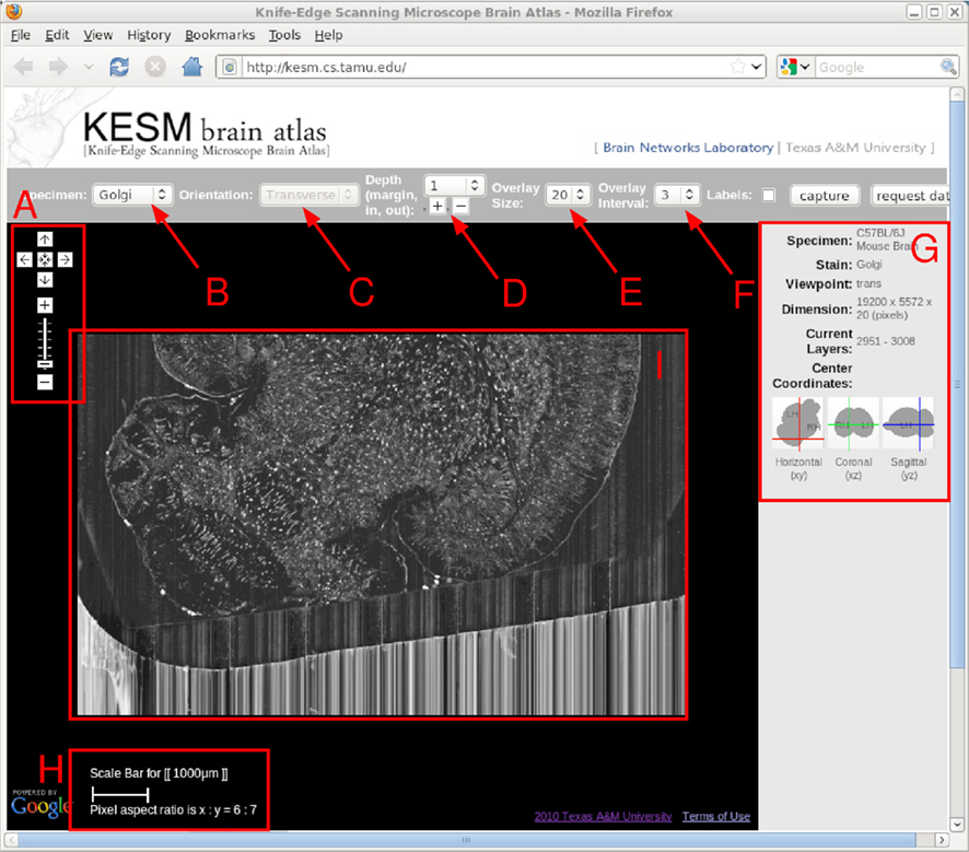
Figure 4. KESM brain atlas interface. A screenshot of the KESM brain atlas running in a web browser is shown. Red markers and text were added on top for the purpose of explanation, below. (A) Navigation panel: panning and zoom-in/zoom-out. (B) Data set selection. Golgi, Golgi2, India Ink are available in the pull-down menu. (C) Sectioning plane orientation. Three standard planes supported (planned). (D) Depth navigation. Amount of movement (unit = 1 μm) in the z direction and forward (deeper, [+]) or backward (shallower, [−]) can be controlled. (E) Overlay count. How many images to overlay can be selected here. (F) Overlay interval. For high zoom-out levels, overlaying every n images is enough, and this helps visualize thicker sections. (G) Information window containing specimen meta data and current location information. (H) Scale bar that automatically adjust to the given zoom level. (I) Main display. Note that the Google logo on the bottom left is shown due to the use of the Google Maps API, and it by no means indicate any connection between the KESM data and Google.
3. Results
In this section, we will present our two KESM Golgi data sets and results from applying the KESMBA framework to these data sets.
3.1. KESM Golgi Data Sets
The first Golgi brain was sectioned and imaged in 2008 (from July 7 to August 8, 2008). These results were first reported in Abbott (2008). The first Golgi data set did not include the left frontal lobe, part of the left temporal lobe, and part of the right frontal lobe due to a misconfigured frame buffer that truncated the images, although the entire brain was sectioned using the KESM. The second Golgi brain was sectioned and imaged in 2010 (from June 8 to August 4, 2010). The second data set contained the entire brain. The first Golgi data set, although partly incomplete, includes less noise than the second Golgi data set, so we decided to make available both data sets within the KESMBA framework. These results are shown in Figures 5–7. All data sets had a voxel resolution of 0.6 μm × 0.7 μm × 1.0 μm, so at maximum zoom, the data are quite detailed, as shown in Figure 8.
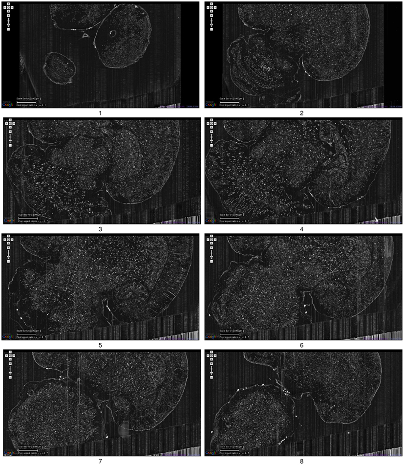
Figure 5. Golgi data set 1. A fly-through of the Golgi data set 1 is shown. The data were obtained by sectioning in the horizontal plane (upper right corner: anterior, lower left corner: posterior). This is the full extent of the data that was captured. We can see that part of the left temporal lobe, left frontal lobe, and part of the right frontal lobe are cut off. Scale bar = 1 mm. Each image is an overlay of 20 images in the z direction. The z-interval between each panel is 600 μm. The numbers below the panels show the ordering. These are cropped screenshots from the KESMBA. This data set, obtained in 2008, is the first whole-brain-scale data set of the mouse at sub-micrometer resolution.
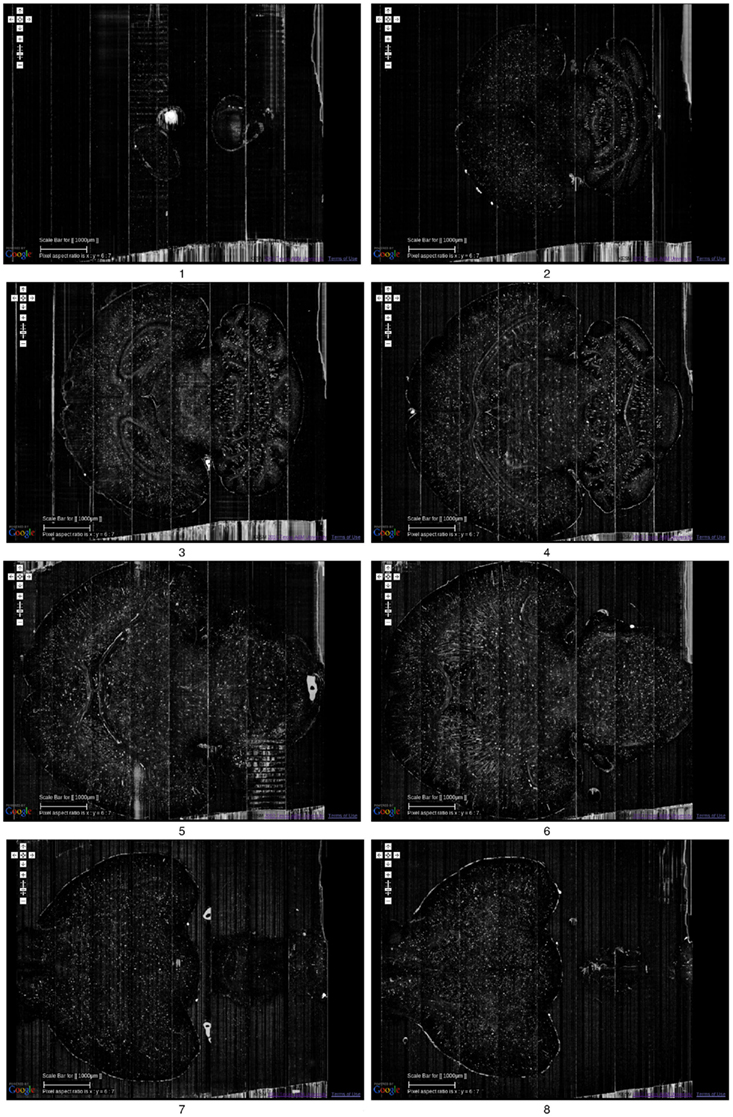
Figure 6. Golgi data set 2. A fly-through of the Golgi data set 2 is shown. The data were obtained by sectioning in the horizontal plane (left: anterior, right: posterior). Scale bar = 1 mm. Each image is an overlay of 20 images in the z direction. The z-interval between each panel is 800 μm, except for the last where it was 200 μm (so that data from near the bottom of the data stack can be shown: otherwise it will overshoot into regions with no data). The numbers below the panels show the ordering. See Movie S1 in Supplementary Material for a fly-through of this data set.
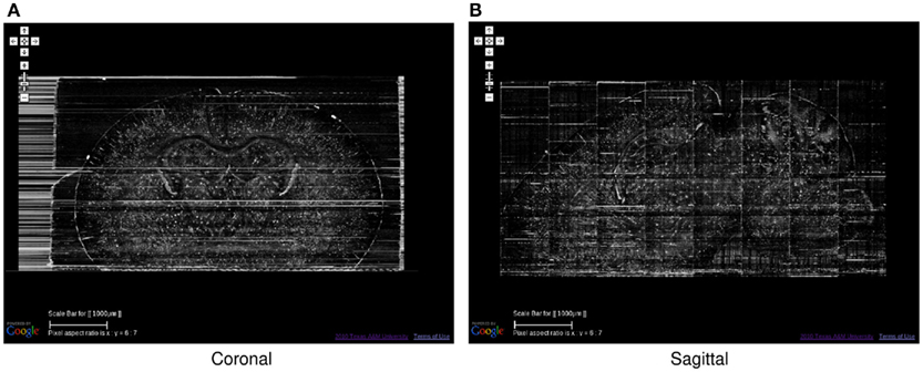
Figure 7. Golgi data set 2, Coronal and Sagittal Views. The coronal (A) and sagittal (B) views of the data set in Figure 6 are shown. Scale bar = 1 mm. These views show the superior z-axis resolution of the KESM data sets.
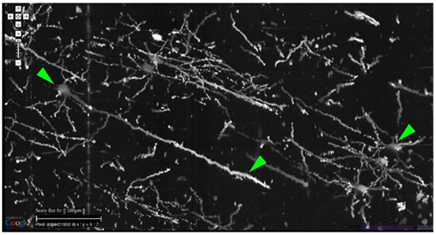
Figure 8. Details from Golgi data set 1. Details from the Golgi data set 1 are shown at full resolution. This panel shows an overlay of 20 images, thus it is showing a 20-μm-thick volume. Scale bar = 100 μm. The arrow heads, from left to right, point to (1) the soma of a pyramidal cell in the cortex and (2) its apical dendrite, and (3) a couple of spiny stellate cells. Other pyramidal cells and stellate cells can be seen in the background. At this resolution, we can see dendritic spines as well.
3.2. 3D Rendering through Image Overlays
All results shown in Figures 5–8 were from direct screenshots of the KESMBA. The 3D effect is most notable in Figure 8. To highlight the z-axis resolution of the KESM data sets, and to show the effectiveness of our overlaying technique, we prepared views of a fixed region in the KESM data set by varying the number of overlays (Figures 9A–C). As we can see from this figure, overlays are effective in rendering 3D content, all within a standard web browser without any dedicated plug-in. Another technique that we implemented that is especially helpful when viewing with a larger field of view (i.e., zoomed out) is to overlay images at a certain interval. For example, overlaying 20 images at an interval of 5 would visualize a 100-μm-thick volume (compare Figures 9D,E).
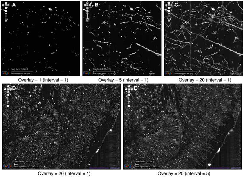
Figure 9. Effectiveness of image overlays. The effect of an increasing number of overlays is shown. Scale bar = 100 μm. The data is from the same region as that from Figure 8. (A) Since each KESM image corresponds to a 1-μm-thick section, a single image conveys little information about the neuronal morphology. (B) Five overlayed images, corresponding to a 5-μm-thick section, begins to show some structure but it is not enough. (C) With twenty overlayed images, familiar structures begin to appear. (D,E) At a zoomed-out scale, skipping over images can be an effective strategy to view the circuits more clearly. In (D), 20 overlays at an interval of 1, representing a 20-μm-thick volume is shown. In (E), 20 overlays at an interval of 5 is shown, representing 100 μm. The dense dendritic arbor in the hippocampus (left), fiber tract projecting toward the hippocampal commissure (middle, top), and the massive number of pyramidal cells and their apical dendrites (right) are clearly visible only in (E).
3.3. Multiscale Nature of the KESM Data
One of the main advantages of the KESMBA is that it is very easy to navigate through the data, both within a certain scale and across multiple scales. In fact, this capability assisted greatly in producing the figures in the very article. Here, we will present the multiscale nature of the KESM data and show the effectiveness of the KESMBA framework in handling such multiscale data. In Figure 10, we show successive snapshots of the KESMBA while zooming from the largest scale to the smallest scale. Each step of zooming in doubles the resolution, so the final panel has 32× higher resolution than the first panel.
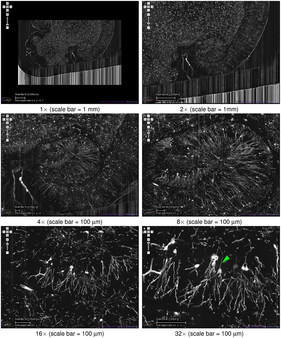
Figure 10. Multiscale view of the KESMBA. A multiscale view of the KESMBA is shown (Golgi data set 1), by gradually zooming into the hippocampus (the numbers below the panels show the zoom-in sequence). All panels show an overlay of 20 sections. The first four panels are shown with an overlay interval of 5 and the last two with an interval of 1. Axons emerging from the hippocampal neurons are clearly visible (arrow head, last panel).
3.4. Neuronal Circuits: Local and Global
Finally, we examine the relevance of the KESM data sets to connectomics research. Although it is true that with Golgi-Cox only ∼1% of the entire population of neurons are stained and thin myelinated axons are not stained reliably, we can still gain valuable insights from this whole-organ level data at a microscopic resolution.
KESM Golgi data sets can help advance connectomics research in two ways, (1) locally and (2) globally. At the local scale, we can investigate the basic circuits (Shepherd, 2003). Although exact connectivity cannot be established, the repeating pattern can help us refine our basic circuit model, and also use the data to validate synthetic circuits constructed based on a theoretical generative model (see, e.g., van Pelt and Uylings, 2005; Koene et al., 2009). Having access to these basic circuits from all regions in the brain is also a great benefit, as shown in Figure 11. This figure shows neurons from the cerebellum, inferior colliculus, thalamus, and hippocampus.
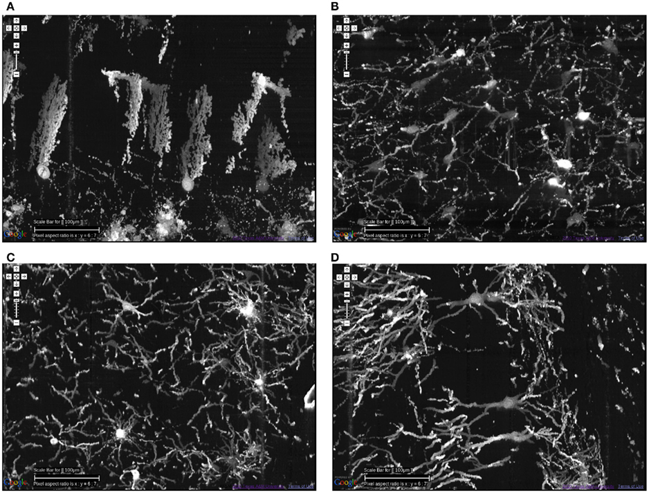
Figure 11. Different types of local circuits. Different types of local circuits from the KESM Golgi data set 1 are shown. (A) Cerebellum. (B) Inferior colliculus. (C) Thalamus. (D) Hippocampus (also see Figure 10). See Figure 8 for circuits in the neocortex. Scale bar = 100 μm. See Movie 2 in Supplementary Material (cerebellum, colliculi) and Movie 3 in Supplementary Material (hippocampus).
At the global scale, certain fiber tracts show up prominently in the KESM Golgi data. For example, various commissures in the frontal lobe and dense fiber bundles in the striatum are prominently visible (Figure 12). Similar fiber tracts can easily be identified, such as the hippocampal commissure in the posterior part of the brain.
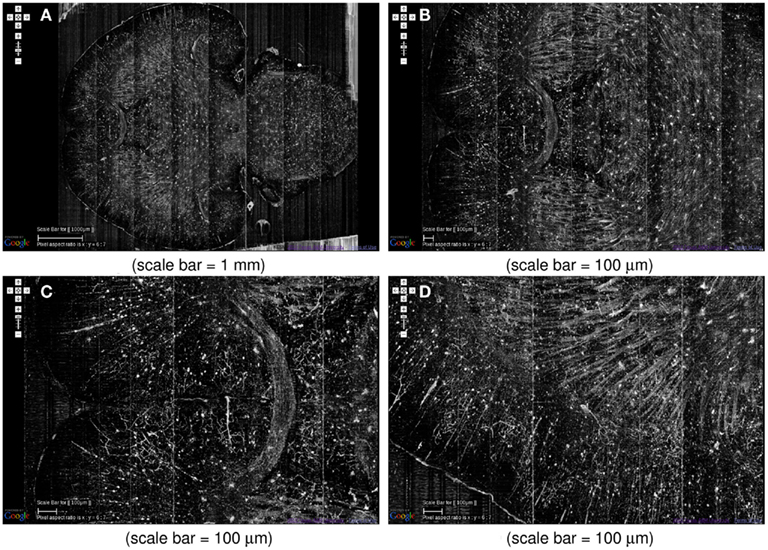
Figure 12. System-level fiber tracts in the KESM Golgi data set 2. (A) Horizontal section at the level of the anterior commissure (the “)”-shaped fiber bundle) is shown (left: anterior, right: posterior). Massive fiber tracts in the striatum can also be observed. (B,C) Zoomed in view showing the anterior commissure near the middle. (D) Close-up of the fiber bundles in the striatum can be seen. A large number of apical dendrites in the adjoining cortex can also be seen.
3.5. Download Performance
The above results confirm the effectiveness of the KESMBA’s pseudo 3D view method using image overlays. However, the additional image overlays mean longer download time, and it will have limited utility if the download time exceeds waiting time tolerable for the users. Figure 13 shows the result of download time analysis of the KESMBA. Download time and download data size were measured in two modern web browsers (Internet Explorer 8.0.6 and Mozilla Firefox 3.6.8) using HttpWatch 7.0.26, a browser plug-in to monitor http traffic. Expectedly, the download time and data size were proportional to the number of overlays. Notably, Firefox took extraordinarily long with large variance, while downloading 20 overlays. The Intranet and the Internet download times for 20 overlays reached above 22 and 44 s respectively with Microsoft Internet Explorer, and 53 and 52 s respectively with Mozilla Firefox. Literature on the tolerable waiting time for a web page download presents discordant thresholds between 4 and 41 s (Selvidge et al., 2002; Galletta et al., 2004), but none of them used a web page with as much graphical content as the KESMBA. Considering the unique graphics-rich nature of the KESMBA, we believe the above download times are within the tolerable threshold.
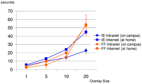
Figure 13. KESMBA download performance analysis. Average of 10 download trials for each setting (browser type and overlay size) is plotted (error bars indicate standard deviation). IE, internet explorer, FF, firefox. Except for the case of Mozilla Firefox downloading 20 overlays, both the Intranet and Internet downloading times increased proportionally with the overlay size.
4. Discussion
This article presents one of the first whole-brain-scale mouse brain atlases imaged at a sub-micrometer resolution, and a novel neuroinformatics framework for rapid visualization and exploration of the massive data sets. The main value of this kind of resource is that it fills the gap between (1) the lower resolution (100s of μms), system-level (10s of cm), diffusion MRI-based tractography data and (2) the higher resolution (10s of nm), small volume (10s of μm), EM-based synaptome data. Both local and global circuit data from our KESM brain atlas are expected to contribute greatly to connectomics research. In the following, we will discuss existing brain atlas and neuronal morphology resources and draw a comparison with the KESM brain atlas, and consider potential challenges and initial solutions.
4.1. Brain Maps and Atlases
The 3D mouse brain atlas, at a typical macroscale spatial resolution of 10 μm, is an indispensable guide to navigation within the mouse brain (Paxinos and Franklin, 2001; Paxinos and Watson, 2006). Without it, the mouse brain microstructure, viewed as a database of individual neurons, is virtually unintelligible. The focus of activity for standardizing anatomical structures and ontology for the mouse, like those defined in the mouse and rat atlases produced by Paxinos and Franklin (2001) and Paxinos and Watson (2006), are at this macrostructure level.
4.1.1. The mouse atlas project (MAP)
MacKenzie-Graham et al. (2003) developed a probabilistic atlas of the adult and developing C57BL/6J mouse. MAP consists of not only data from Magnetic Resonance Microscopy (MRM) and histological atlases, but also a suite of tools for image processing, volume registration, volume browsing, and annotation. MAP will produce an imaging framework to house and correlate gene expression with anatomic and molecular information drawn from traditional and novel imaging technologies. This digital atlas of the C57BL/6J mouse brain is composed of volumes of data acquired from μMRI, block-face imaging, histology, and immunohistochemistry. MAP technology provides the infrastructure for the development of the Allen Brain Atlas (MacKenzie-Graham et al., 2003; see below). Also see the related Mouse BIRN (Biomedical Informatics Research Network).
4.1.2. The allen brain atlas
The Allen Brain Atlas contains detailed gene expression maps for ∼20,000 genes in the C57BL/6J mouse (Lein et al., 2007). A semi-automated procedure was used to conduct in situ hybridization and data acquisition on 25 μm-thick sections (z-axis) of the mouse brain. The x-y-axis resolution of the images range from 0.95 to 8 μm. The Allen Brain Atlas is the first comprehensive gene expression map at the whole-brain level, and is currently accessed over 4 million times per month, with over 250 scientists browsing the data on a daily basis.
4.1.3. The mouse brain library (MBL)
MBL is developing methods to construct atlases from celloidin-embedded tissue to guide registration of MBL data into a standard coordinate system, by segmenting each brain in its collection into 1,200 standard anatomical structures at a resolution of 36 μm (Rosen et al., 2000). Algorithms are to be designed to segment each brain in the MBL into a set of standard anatomical structures like those defined in the rat atlas produced by Computer Vision Laboratory for Vertebrate Brain Mapping at Drexel College of Medicine, whose computerized 3D atlas was built from stained sections for the mouse brain that reconstructs Nissl-stained sectional material, a 17.9-μm isotropic 3D data set, from a freshly frozen brain of an adult male C57BL/6J mouse.
4.1.4. BrainMaps.org
BrainMaps.org is an internet-enabled, high-resolution brain map (Mikula et al., 2007). The map contains over 10 million mega pixels (35 terabytes) of scanned data, at a typical resolution of ∼0.46 μm/pixel (in the x-y plane). The atlas provides an intuitive web-based interface for easy and band-width-efficient navigation, through the use of a series of subsampled (zoomed out) views of the data sets, similar to the Google Maps interface. Even though the x-y plane resolution is below 1 μm, the z-axis resolution is orders of magnitude lower (for example, one coronal brain set has 234 slides in it, corresponding to a sectional thickness of 25 μm). The database also serves serial sections from electron microscopy, cryo sections, and immunohistochemistry, and hosts a total of 135 data sets (as of March 2, 2011).
4.1.5. Whole-brain catalog (WBC)
WBC is a 3D virtual environment for exploring multiple sources of brain data (including mouse brain data), e.g., Cell Centered Database (CCDB, see below), Neuroscience Information Framework (NIF), and the Allen Brain Atlas (see above). WBC has native support for registering to the Waxholm Space, a rodent standard atlas space (Johnson et al., 2010). Multiple functionalities including visualization, slicing, animations, and simulations are supported.
In summary, there are several mouse brain atlases available, with data from different imaging modalities, but their resolution is not high enough in one or more of the x, y, or z axes to show morphological detail of neurons.
4.2. Databases of 3D Reconstruction of Neurons
The low spatial resolution in existing whole-brain level brain maps and atlases have been pointed out as a major limitation. Near-micron-level reconstructions of brain areas do exist, but only for a small volume. Part of the reason is that, in many cases, the geometric reconstructions were done manually, with the aid of interactive editing tools like Neurolucida (Glaser and Glaser, 1990), Reconstruct (Fiala, 2005), or Neuron_Morpho (Brown et al., 2007).
4.2.1. The Duke/Southampton archive of neuronal morphology
This on-line archive of neuronal geometry (Cannon et al., 1998) includes full 3D representations of 124 neurons from the rat hippocampus, obtained following intracellular staining with biocytin and reconstruction using Neurolucida. The archive includes data both in the native format as supplied from the digitization software, and in a simpler, 3D standardized format (given the extension “SWC” in the archive). The data for the SWC files are obtained by fitting cell segments in three dimensions with cylinders, directly confirming the location and size of these shapes using a computer-based tracing system.
4.2.2. NeuroMorpho.org
This is a centrally curated collection of reconstructed neurons, currently containing 5793 cells (version 5, November 15, 2010) from various species and brain regions (Ascoli et al., 2007). The data are available for download in SWC format. L-neuron is a modeling and analysis project that is associated with this database, where statistical features of dendritic geometry and stochastic generation of (statistically) realistic neurons are studied (Senft and Ascoli, 1999; Ascoli and Krichmar, 2000; Ascoli, 2002).
4.2.3. The cell centered database (CCDB)
CCDB houses high-resolution 3D light and electron microscopic reconstructions spanning the dimensional range from 5 nm3 to 50 μm3 produced at the National Center for Microscopy and Imaging Research (NCMIR; Martone et al., 2002). The current CCDB has 8391 micrograph data sets (as of March 2, 2011) in various modalities including confocal, light microscopy, electron tomography, electron microscopy, live imaging, filled cell imaging, protein imaging, and serial block-face imaging.
4.2.4. The SynapseWeb
The SynapseWeb (Fiala and Harris, 2001) is a portal into a dense network of synaptic connections and supporting structures in the gray matter of the brain that can be fully visualized only through 3D electron microscopy. It provides an interface for examining volumes of brain tissue at nanometer resolutions which have been reconstructed from serial section electron microscopy. Currently, the SynapseWeb houses three brain volumes ranging from 62 to 108 μm3 from the CA1 regions of rat hippocampus.
In summary, there are several excellent neuronal morphology databases that serve the neuroscience community, but they are limited to a small number of neurons from limited volumes, isolated from the system-level context.
4.3. Atlasing and Neuronal Morphology Description Standards
A rapid increase in web-based resources serving neuronal morphology and atlas-scale data sets gave rise to the need for data representation standards.
The Waxholm Space (Johnson et al., 2010; Hawrylycz et al., 2011) is a new standard atlasing space for rodents. The effort to build this standard space was motivated by multiple non-standard, yet widely used coordinate spaces such as those in the Allen Brain Atlas (Lein et al., 2007) or Paxinos and Franklin’s atlas (Paxinos and Franklin, 2001).
As for neuronal morphology, NeuroML has become the de facto standard (using XML). BrainML, on the other hand, provides an XML framework for the exchange of general neuroscience data at the whole-brain scale.
4.4. Alternative Mapping APIs
Geospatial interfaces have undergone massive innovation in the last decade and as we have demonstrated in this article, they can be very effective in presenting biological data. However, existing tools are encumbered by proprietary licensing, which limits adaptation to cosmetic levels and requires awkward workarounds to implement even basic functionality. Use of open source tools will allow for code level adaptation as opposed to API extension, and facilitate interoperability and adoption by other groups.
Tools that can help this transition include GDAL and OpenLayers. The open source GDAL1 is a translator library for data formats maintained by the Open Source Geospatial Foundation. OpenLayers is an open source browser-based map display system using client side JavaScript. OpenLayers2 serves up data as a service and supports the basic tile display functionality (i.e., zoom levels, layers) with custom controls used in map navigation. It also supports a number of advanced features such as layer opacity, feature opacity, vector formats and others necessary for more sophisticated user interfaces. A key feature is the ability to use disk-based caching to improve local performance, which can greatly improve performance of KESMBA-like web atlases.
Open standards and best practices are widely used in the geospatial community and contribute significantly to the interoperability of geospatial visualization across a wide range of devices. Modifications of standards such as the Web Map Service for large scale microscopy data offer potential for interoperability between neuroinformatics systems.
4.5. Challenges
The KESM data sets are in a unique strategic position to help advance the field of connectomics in the short term future (5–10 years). This is due to its system-level scope combined with sub-micrometer resolution. However, there are many challenges that need to be overcome in order to enable fully quantitative connectivity analysis such as graph theoretical analysis (Sporns, 2002; Sporns and Tononi, 2002; Kötter and Stephan, 2003) or motif analysis (Milo et al., 2002). Here, we will discuss some of these challenges and suggest strategies to overcome these challenges.
4.5.1. Establishing connectivity
One of the main issues with any approach based on light microscopy (LM) is the requirement that sparse stains like Golgi are used (which stains about 1% of the total neuronal population). Dense stains commonly used in electron microscopy will render objects in the specimen indistinguishable at the resolution permitted by LM. Furthermore, stains like Golgi do not stain thin axons, thus tracing long projections even for the sparse sample is difficult. Long-range tracers like biocytin could be a good solution, but these tracers require intracellular injection and a long transport time, so applying them at the whole-brain scale can be troublesome. An attractive possibility is to use Brainbow transgenic mice (Livet et al., 2007), combined with fluorescence imaging (recently, we have successfully imaged fluorescent proxies [10 μm beads] with the KESM using laser illumination). This way, neurons are densely labeled, but due to the variation in the emitted wavelength, even close-by neurons can be differentiated (Lichtman et al., 2008). Techniques using pseudorabies virus (PRV) can also be used to label neurons that form an actual circuit since PRV allows for trans-synaptic tracing (Smith et al., 2000; Willhite et al., 2006; Kim et al., 2011). As most recent labeling methods such as Brainbow and PRV require fluorescence imaging, further development of KESM fluorescence imaging capability will become a key requirement.
An alternative to the experimental techniques above is to estimate connectivity based on the sparse data. Methods like those proposed by Kalisman et al. (2003) can be used for this purpose. Also, a systematic simulation study can be conducted with a full synthetic circuit, by dropping a certain proportion of connections and observing the resulting change in behavior. The degree of redundancy in the connections (both for real and synthetic circuits) will play an important role here.
4.5.2. From image to structure
Another important issue is that of structural reconstruction (Figure 14). Together with whole-brain-scale data acquisition, structural reconstruction is a grand challenge for connectomics. The DIADEM (Digital Reconstruction of Axonal and Dendritic Morphology) Challenge and lessons learned from the first round of competition show a long road ahead of us in terms of accurate circuit tracing (Liu, 2011). The KESM data sets are basically image stacks and they do not provide quantitative morphological or connectivity data. Among different approaches we have found that vector tracing methods are fast and reliable (Can et al., 1999; Al-Kofahi et al., 2002; Mayerich et al., 2008a, 2011a; Han et al., 2009a,b). However, these approaches are not perfect and small errors can lead to topological mistakes, which can cause serious errors in establishing connectivity (Jain et al., 2010a). Jain et al. (2010b) propose the use of machine learning techniques, and this can be a promising direction. However, whatever automated methods we use the burden of validation (see, e.g., Warfield et al., 2004; Mayerich et al., 2008c) still remains and human intervention is inevitable. The question is how to make this human intervention minimal while maximizing accuracy. We are currently exploring several options: (1) multiple-choice selection from parameterized reconstruction alternatives, (2) interactive editing using graph cuts, and (3) colorized voxel-intensity-based confidence to aid in rapid editing region selection (Yang and Choe, 2009). These approaches can help combine automated reconstruction algorithms with the power of human computing (von Ahn, 2006; von Ahn et al., 2006, 2008), to enable reliable tracing of massive volumes of neuronal circuit data.
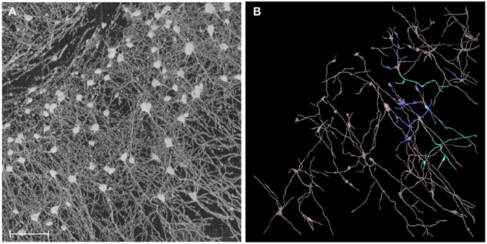
Figure 14. From image to geometry. (A) A portion of KESM Golgi data set 1 is shown (cortex). Maximum intensity projection is used to show a thicker section containing a large number of neurons. Scale bar = 100 μm. (B) Semi-automated 3D reconstruction results are shown (partial results, using Neuromantic, Myatt and Nasuto, 2007).
4.5.3. From structure to function
The connectome is fundamentally a static structure, an adjacency matrix. Important physiological parameters such as sign (excitatory/inhibitory), weight (synaptic efficacy), and delay (axonal conduction delay) are not available. How can these and other physiological properties be inferred from just the structure? Toledo-Rodriguez et al. (2004) shows a possibly powerful solution to this: Use gene expression data. They found that gene expression and electrophysiological properties are closely correlated. The availability of very large gene expression atlases such as the Allen Brain Atlas (Lein et al., 2007; 22,000 genes), and imaging modalities such as Array Tomography that support molecular as well as EM imaging (Micheva and Smith, 2007) are great resources for this kind of approach (see, e.g., Markram, 2006). Another straight-forward yet potentially valuable approach is to start with computational simulation based on detailed neuronal morphology (cf. the Blue Brain Project; Markram, 2006). The reconstructed geometry can be used to construct multi-compartment models (see, e.g., Dayan and Abbott, 2001). Appropriate parameters such as channel conductance, capacitance, etc., need to be figured out (Vanier and Bower, 1999). Tools like NEURON, GENESIS, neuroConstruct, and NeuGEN can be used for multi-compartment simulation and parameterized synthetic circuit generation/simulation/analysis (Hines and Carnevale, 1997; Bower and Beeman, 1998; Ascoli et al., 2001; Eberhard et al., 2006; Gleeson et al., 2007; Koene, 2007; Koene et al., 2009). Data from the KESM can help narrow down on the range of various parameters for these simulations (see Druckmann et al., 2008 for parameter constraining procedures).
4.5.4. Enabling connectomics research through neuroinformatics
From visualization to annotation to editing and quantitative analysis, neuroinformatics tools are expected to serve as a key to the success of connectomics research. This is because the process of going from data to information and information to knowledge cannot be achieved through purely automated (fast but inaccurate) or purely manual (accurate but slow) means. Thus, an informatics platform is needed to optimally blend both automated and manual exploration and analysis methods.
The KESM brain atlas framework provides a good starting point. However, to increase its utility as a connectomics platform, it needs to be expanded to include support for all three standard sections (coronal, horizontal, and sagittal), overlay of automated reconstructions, and reconstruction editing facilities (uncertainty/confidence visualization, reconstruction alternatives, etc.). These reconstructed morphologies have to be moved one step farther to achieve the connectivity diagram needed for connectomics research. Thus, facilities to allow users to manually specify neuron-to-neuron connectivity, or allow parametric connectivity specification (e.g., connect axons and dendrites that meet a certain rule, where the rule can be specified by setting parameters such as proximity radius, etc.) are needed. With the reconstructed geometry already in place, calculating such parameterized connectivity could be done rapidly. A distribution of connection matrices can be generated based on such parametrizations, from which meaningful structural and functional properties of the connectome can be extracted.
Conflict of Interest Statement
Todd Huffman is employed by 3Scan. Part of the instrumentation, computing, and storage costs of this project has been funded by 3Scan.
Acknowledgments
This project was funded in part by the Collaborative Research in Computational Neuroscience Program of National Science Foundation (NSF CRCNS #0905041), National Institutes of Health - National Institute of Neurological Disorders and Stroke (NIH/NINDS #1R01-NS54252), the National Science Foundation’s (NSF) Major Research Instrumentation (MRI) Program (NSF MRI #0079874), the National Science Foundation’s (NSF) Information Technology Research (ITR) Program (NSF ITR #CCR-0220047), Texas Higher Education Coordinating Board (ATP#000512-0146-2001), Texas A&M Research Foundation, Texas Engineering Experiment Station, and 3Scan. The appearance of the Google logo in the figures are due to the use of the Google Maps API by the KESM brain atlas. Besides that this work was done independent of Google. We would like to thank Bruce H. McCormick, inventor of the KESM, for his visionary insights, and Bernard Mesa for technical advice and instrumentation for the KESM.
Supplementary Material
The Movies S1, S2, and S3 for this article can be found online at http://www.frontiersin.org/Neuroinformatics/10.3389/fninf.2011.00029/abstract
Media Files: All video clips were made using MeVisLab (http://www.mevislab.de). Note that the video clips are presented to showcase the KESM data itself, and are independent of the KESMBA web interface.
Movie S1. video clip of a sweep-through of the entire KESM Golgi data set 2 is shown, along all three sectioning planes: Sagittal, coronal, and horizontal. Initial block width is 11.52 mm.
Movie S2. A video clip of a small region near the cerebellum and the colliculi from the KESM Golgi data set 1 is shown. Zoom-in near the end of the clip shows a number of cerebellar Purkinje cells. The view is initially horizontal, but later on it rotates and shows sagittal sections. Initial width of the block is 2.88 mm.
Movie S3. A video clip of a small region near the hippocampus (middle) and the cortex (bottom) from the KESM Golgi data set 1 is shown. Initial width of the block is 1.44 mm.
Footnotes
References
Abbott, L. C. (2008). “High-throughput imaging of whole small animal brains with the knife-edge scanning microscope,” in Neuroscience Meeting Planner, Program No. 504.2. Washington, DC: Society for Neuroscience.
Abbott, L. C., and Sotelo, C. (2000). Ultrastructural analysis of catecholaminergic innervation in weaver and normal mouse cerebellar cortices. J. Comp. Neurol. 426, 316–329.
Al-Kofahi, K. A., Lasek, S., Szarowski, D. H., Pace, C. J., Nagy, G., Turner, J. N., and Roysam, B. (2002). Rapid automated three-dimensional tracing of neurons from confocal image stacks. IEEE Trans. Inf. Technol. Biomed. 6, 171–187.
Ascoli, G., Krichmar, J., Scorcioni, R., Nasuto, S., and Senft, S. (2001). Computer generation and quantitative morphometric analysis of virtual neurons. Anat. Embryol. (Berl.) 204, 283–301.
Ascoli, G. A., Donohue, D. E., and Halavi, M. (2007). NeuroMorpho.Org: a central resource for neuronal morphologies. J. Neurosci. 27, 9247–9251.
Ascoli, G. A., and Krichmar, J. L. (2000). L-Neuron: a modeling tool for the efficient generation and parsimonious description of dendritic morphology. Neurocomputing 32–33, 1003–1011.
Ascoli, G. A. (ed.). (2002). Computational Neuroanatomy: Principles and Methods. Totowa, NJ: Humana Press.
Basser, P. J., and Jones, D. K. (2002). Diffusion-tensor MRI: theory, experimental design and data analysis – a technical review. NMR Biomed. 15, 456–467.
Bower, J. M., and Beeman, D. (1998). The Book of GENESIS: Exploring Realistic Neural Models with the General Neural Simulation System. Santa Clara, CA: Telos.
Brown, K. M., Donohue, D. E., D’Alessandro, G., and Ascoli, G. A. (2007). A cross-platform freeware tool for digital reconstruction of neuronal arborizations from image stacks. Neuroinformatics 3, 343–359.
Can, A., Shen, H., Turner, J. N., Tanenbaum, H. L., and Roysam, B. (1999). Rapid automated tracing and feature extraction from retinal fundus images using direct exploratory algorithms. IEEE Trans. Inf. Technol. Biomed. 3, 125–138.
Cannon, R. C., Turner, D. A., Pyapali, G. K., and Wheal, H. V. (1998). An on-line archive of reconstructed hippocampal neurons. J. Neurosci. Methods 84, 49–54.
Choe, Y., Abbott, L. C., Han, D., Huang, P.-S., Keyser, J., Kwon, J., Mayerich, D., Melek, Z., and McCormick, B. H. (2008). “Knife-edge scanning microscopy: high-throughput imaging and analysis of massive volumes of biological microstructures,” in High-Throughput Image Reconstruction and Analysis: Intelligent Microscopy Applications, eds A. R. Rao and G. Cecchi (Boston, MA: Artech House), 11–37.
Choe, Y., Abbott, L. C., Miller, D. E., Han, D., Yang, H.-F., Chung, J. R., Sung, C., Mayerich, D., Kwon, J., Micheva, K., and Smith, S. J. (2010). “Multiscale imaging, analysis, and integration of mouse brain networks,” in Neuroscience Meeting Planner, Program No. 516.3. San Diego, CA: Society for Neuroscience.
Choe, Y., Han, D., Huang, P.-S., Keyser, J., Kwon, J., Mayerich, D., and Abbott, L. C. (2009). “Complete submicrometer scans of mouse brain microstructure: neurons and vasculatures,” in Neuroscience Meeting Planner, Program No. 389.10. Chicago, IL: Society for Neuroscience.
Denk, W., and Horstmann, H. (2004). Serial block-face scanning electron microscopy to reconstruct three-dimensional tissue nanostructure. PLoS Biol. 19, e329. doi:0.1371/journal.pbio.0020329
Druckmann, S., Berger, T. K., Hill, S., Schürmann, F., Markram, H., and Segev, I. (2008). Evaluating automated parameter constraining procedures of neuron models by experimental and surrogate data. Biol. Cybern. 99, 371–379.
Eberhard, J. P., Wanner, A., and Wittum, G. (2006). NeuGen: a tool for the generation of realistic morphology of cortical neurons and neural networks. Neurocomputing 70, 327–342.
Eng, D. C.-Y., and Choe, Y. (2008). “Stereo pseudo 3D rendering for web-based display of scientific volumetric data,” in Proceedings of the IEEE/EG International Symposium on Volume Graphics. Los Angeles, CA.
Fiala, J. C. (2005). Reconstruct: a free editor for serial section microscopy. J. Microsc. 218, 52–61.
Fiala, J. C., and Harris, K. M. (2001). Extending unbiased stereology of brain ultrastructure to three-dimensional volumes. J. Am. Med. Inform. Assoc. 8, 1–16.
Galletta, D. F., Henry, R., McCoy, S., and Polak, P. (2004). Web site delays: how tolerant are users? J. Assoc. Inf. Syst. 5, 1–28.
Glaser, J. R., and Glaser, E. M. (1990). Neuron imaging with Neurolucida – a PC-based system for image combining microscopy. Comput. Med. Imaging Graph. 14, 307–317.
Gleeson, P., Steuber, V., and Silver, R. (2007). NeuroConstruct: a tool for modeling networks of neurons in 3D space. Neuron 54, 219–235.
Hagmann, P., Kurant, M., Gigandet, X., Thiran, P., Wedeen, V. J., Meuli, R., and Thiran, J.-P. (2007). Mapping human whole-brain structural networks with diffusion MRI. PLoS ONE 2, e597. doi:10.1371/journal.pone.0000597
Han, D., Choi, H., Park, C., and Choe, Y. (2009a). “Fast and accurate retinal vasculature tracing and kernel-isomap-based feature selection,” in Proceedings of the International Joint Conference on Neural Networks (Piscataway, NJ: IEEE Press), 1075–1082.
Han, D., Keyser, J., and Choe, Y. (2009b). “A local maximum intensity projection tracing of vasculature in knife-edge scanning microscope volume data,” in Proceedings of the IEEE International Symposium on Biomedical Imaging, Boston, MA, 1259–1262.
Hawrylycz, M., Baldock, R. A., Burger, A., Hashikawa, T., Johnson, G. A., Martone, M., Ng, L., Lau, C., Larsen, S. D., Nissanov, J., Puelles, L., Ruffins, S., Verbeek, F., Zaslavsky, I., and Boline, J. (2011). Digital atlasing and standardization in the mouse brain. PLoS Comput. Biol. 7, e1001065. doi:10.1371/journal.pcbi.1001065
Hayworth, K. (2008). “Automated creation and SEM imaging of Ultrathin Section Libraries: tools for large volume neural circuit reconstruction,” in Society for Neuroscience Abstracts, Program No. 504.4. Washington, DC: Society for Neuroscience.
Hines, M. L., and Carnevale, N. T. (1997). The NEURON simulation environment. Neural. Comput. 9, 1179–1209.
Jain, V., Bollmann, B., Richardson, M., Berger, D. R., Helmstaedter, M. N., Briggman, K. L., Denk, W., Bowden, J. B., Mendenhall, J. M., Abraham, W. C., Harris, K. M., Kasthuri, N., Hayworth, K. J., Schalek, R., Tapia, J. C., Lichtman, J. W., and Seung, H. S. (2010a). “Boundary learning by optimization with topological constraints,” in Proceedings of the IEEE Conference on Computer Vision and Pattern Recognition, San Francisco, CA, 2488–2495.
Jain, V., Seung, H. S., and Turaga, S. C. (2010b). Machines that learn to segment images: a crucial technology for connectomics. Curr. Opin. Neurobiol. 20, 653–666.
Johnson, G. A., Badea, A., Brandenburg, J., Cofer, G., Fubara, B., Liu, S., and Nissanov, J. (2010). Waxholm space: an image-based reference for coordinating mouse brain research. Neuroimage 53, 365–372.
Kalisman, N., Silberberg, G., and Markram, H. (2003). Deriving physical connectivity from neuronal morphology. Biol. Cybern. 88, 210–218.
Kersten, M., Stewart, J., Troje, N., and Ellis, R. (2006). Enhancing depth perception in translucent volumes. IEEE Trans. Vis. Comput. Graph 12, 1117–1124.
Kim, D. H., Phillips, M. E., Chang, A. Y., Patel, H. K., Nguyen, K. T., and Willhite, D. C. (2011). Lateral connectivity in the olfactory bulb is sparse and segregated. Front. Neural Circuits, 5:5. doi:10.3389/fncir.2011.00005
Koene, R. A. (2007). “Large scale high resolution network generation: producing known validation sets for serial reconstruction methods that use histological images of neural tissue,” in International Conference on Complex Systems. Boston, MA. [Presentation].
Koene, R. A., Tijms, B., van Hees, P., Postma, F., de Ridder, A., Ramakers, G. J. A., van Pelt, J., and van Ooyen, A. (2009). NETMORPH: a framework for the stochastic generation of large scale neuronal networks with realistic neuron morphologies. Neuroinformatics 7, 1539–2791.
Kötter, R., and Stephan, K. E. (2003). Network participation index: characterizing component roles for information processing in neural networks. Neural Netw. 16, 1261–1275.
Kwon, J., Mayerich, D., Choe, Y., and McCormick, B. H. (2008). “Lateral sectioning for knife-edge scanning microscopy,” in Proceedings of the IEEE International Symposium on Biomedical Imaging, Paris, France, 1371–1374.
Lein, E. S., Hawrylycz, M. J., Ao, N., Ayres, M., Bensinger, A., Bernard, A., Boe, A. F., Boguski, M. S., Brockway, K. S., Byrnes, E. J., Chen, L., Chen, L., Chen, T. M., Chin, M. C., Chong, J., Crook, B. E., Czaplinska, A., Dang, C. N., Datta, S., Dee, N. R., Desaki, A. L., Desta, T., Diep, E., Dolbeare, T. A., Donelan, M. J., Dong, H. W., Dougherty, J. G., Duncan, B. J., Ebbert, A. J., Eichele, G., Estin, L. K., Faber, C., Facer, B. A., Fields, R., Fischer, S. R., Fliss, T. P., Frensley, C., Gates, S. N., Glattfelder, K. J., Halverson, K. R., Hart, M. R., Hohmann, J. G., Howell, M. P., Jeung, D. P., Johnson, R. A., Karr, P. T., Kawal, R., Kidney, J. M., Knapik, R. H., Kuan, C. L., Lake, J. H., Laramee, A. R., Larsen, K. D., Lau, C., Lemon, T. A., Liang, A. J., Liu, Y., Luong, L. T., Michaels, J., Morgan, J. J., Morgan, R. J., Mortrud, M. T., Mosqueda, N. F., Ng, L. L., Ng, R., Orta, G. J., Overly, C. C., Pak, T. H., Parry, S. E., Pathak, S. D., Pearson, O. C., Puchalski, R. B., Riley, Z. L., Rockett, H. R., Rowland, S. A., Royall, J. J., Ruiz, M. J., Sarno, N. R., Schaffnit, K., Shapovalova, N. V., Sivisay, T., Slaughterbeck, C. R., Smith, S. C., Smith, K. A., Smith, B. I., Sodt, A. J., Stewart, N. N., Stumpf, K. R., Sunkin, S. M., Sutram, M., Tam, A., Teemer, C. D., Thaller, C., Thompson, C. L., Varnam, L. R., Visel, A., Whitlock, R. M., Wohnoutka, P. E., Wolkey, C. K., Wong, V. Y., Wood, M., Yaylaoglu, M. B., Young, R. C., Youngstrom, B. L., Yuan, X. F., Zhang, B., Zwingman, T. A., and Jones, A. R. (2007). Genome-wide atlas of gene expression in the adult mouse brain. Nature 445, 168–176.
Li, A., Gong, H., Zhang, B., Wang, Q., Yan, C., Wu, J., Liu, Q., Zeng, S., and Luo, Q. (2010). Micro-optical sectioning tomography to obtain a high-resolution atlas of the mouse brain. Science 330, 1404–1408.
Lichtman, J. W., Livet, J., and Sanes, J. R. (2008). A technicolour approach to the connectome. Nat. Rev. Neurosci. 9, 417–422.
Livet, J., Weissman, T. A., Kang, H., Draft, R. W., Lu, J., Bennis, R. A., Sanes, J. R., and Lichtman, J. W. (2007). Transgenic strategies for combinatorial expression of fluorescent proteins in the nervous system. Nature 450, 56–62.
MacKenzie-Graham, A., Jones, E. S., Shattuck, D. W., Dinov, I. D., Bota, M., and Toga, A. W. (2003). The informatics of a C57BL/6J mouse brain atlas. Neuroinformatics 1, 397–410.
Martone, M. E., Gupta, A., Wong, M., Qian, X., Sosinsky, G., Ludscher, B., and Ellisman, M. H. (2002). A cell-centered database for electron tomographic data. J. Struct. Biol. 138, 145–155.
Mayerich, D., Abbott, L. C., and Keyser, J. (2008a). Visualization of cellular and microvessel relationship. IEEE Trans. Vis. Comput. Graph. 14, 1611–1618.
Mayerich, D., Abbott, L. C., and McCormick, B. H. (2008b). Knife-edge scanning microscopy for imaging and reconstruction of three-dimensional anatomical structures of the mouse brain. J. Microsc. 231, 134–143.
Mayerich, D., Kwon, J., Choe, Y., Abbott, L., and Keyser, J. (2008c). “Constructing high-resolution microvascular models,” in Proceedings of the 3rd International Workshop on Microscopic Image Analysis with Applications in Biology (MIAAB 2008), New York, NY.
Mayerich, D., Bjornsson, C., Taylor, J., and Roysam, B. (2011a). “Metrics for comparing explicit representations of interconnected biological networks,” in IEEE Symposium on Biological Data Visualization, Chicago, IL, 79–86.
Mayerich, D., Kwon, J., Sung, C., Abbott, L. C., Keyser, J., and Choe, Y. (2011b). Fast macro-scale transmission imaging of microvascular networks using KESM. Biomed. Opt. Express 2, 2888–2896.
Mayerich, D., McCormick, B. H., and Keyser, J. (2007). “Noise and artifact removal in knife-edge scanning microscopy,” in Proceedings of the IEEE International Symposium on Biomedical Imaging, Washington, DC, 556–559.
McCormick, B. H. (2003). The knife-edge Scanning Microscope. Technical report, Department of Computer Science, Texas A&M University. Available at: http://research.cs.tamu.edu/bnl/
McCormick, B. H. (2004). U.S. Patent No. 6,744,572. Washington, DC: U.S. Patent and Trademark Office.
Micheva, K., and Smith, S. J. (2007). Array tomography: a new tool for imaging the molecular architecture and ultrastructure of neural circuits. Neuron 55, 25–36.
Mikula, S., Trotts, I., Stone, J. M., and Jones, E. G. (2007). Internet-enabled high-resolution brain mapping and virtual microscopy. Neuroimage 35, 9–15.
Milo, R., Sen-Orr, S., Itzkovitz, S., Kashtan, N., Chklovskii, D., and Alon, U. (2002). Network motifs: simple building blocks of complex networks. Science 298, 824–827.
Myatt, D., and Nasuto, S. (2007). Three-dimensional reconstruction of neurons with neuromantic. AISB Q. 125, 1–2.
Paxinos, G., and Franklin, K. B. J. (2001). The Mouse Brain in Stereotaxic Coordinates, 2nd Edn. San Diego, CA: Academic Press.
Paxinos, G., and Watson, C. (2006). The Rat Brain in Stereotaxic Coordinates, 6th Edn. San Diego, CA: Academic Press.
Roebroeck, A., Galuske, R., Formisano, E., Chiry, O., Bratzke, H., Ronen, I., Kim, D.-S., and Goebel, R. (2008). High-resolution diffusion tensor imaging and tractography of the human optic chiasm at 9.4 T. Neuroimage 39, 157–168.
Rosen, G. D., Williams, A. G., Capra, J. A., Connolly, M. T., Cruz, B., Lu, L., Airey, D. C., Kulkarni, A., and Williams, R. W. (2000). “The mouse brain library@www.mbl.org,” in Proceedings of the 14th International Mouse Genome Meeting, Narita, C6.
Selvidge, P. R., Chaparro, B., and Bender, G. T. (2002). The world wide wait: effects of delays on user performance. Int. J. Ind. Ergon. 29, 15–20.
Senft, S. L., and Ascoli, G. A. (1999). Reconstruction of brain networks by algorithmic amplification of morphometry data. Lect. Notes Comput. Sci. 1606, 25–33.
Shepherd, G. M. (ed.). (2003). The Synaptic Organization of the Brain, 5th Edn. New York: Oxford University Press.
Smith, B. N., Banfield, B. W., Smeraski, C. A., Wilcox, C. L., Dudek, F. E., Enquist, L. W., and Pickard, G. E. (2000). Pseudorabies virus expressing enhanced green fluorescent protein: a tool for in vitro electrophysiological analysis of transsynaptically labeled neurons in identified central nervous system circuits. Proc. Natl. Acad. Sci. U.S.A. 97, 9264–9269.
Sporns, O. (2002). “Graph theory methods for the analysis of neural connectivity patterns,” in Neuroscience Databases: A Practical Guide, ed. R. Kötter (Boston, MA: Kluwer Publishers), 171–186.
Sporns, O., and Tononi, G. (2002). Classes of network connectivity and dynamics. Complexity 7, 28–38.
Sporns, O., Tononi, G., and Kötter, R. (2005). The human connectome: a structural description of the human brain. PLoS Comput. Biol. 1, e42. doi:10.1371/journal.pcbi.0010042
Swanson, L. W. (2003). Brain Architecture: Understanding the Basic Plan. Oxford: Oxford University Press.
Thiel, A., Schwegler, H., and Eurich, C. W. (2003). Complex dynamics is abolished in delayed recurrent systems with distributed feedback times. Complexity 8, 102–108.
Toledo-Rodriguez, M., Blumenfeld, B., Wu, C., Luo, J., Attali, B., Goodman, P., and Markram, H. (2004). Correlation maps allow neuronal electrical properties to be predicted from single-cell gene expression profiles in rat neocortex. Cereb. Cortex 14, 1310–1327.
Tsai, P. S., Friedman, B., Ifarraguerri, A. I., Thompson, B. D., Lev-Ram, V., Schaffer, C. B., Xiong, Q., Tsien, R. Y., Squier, J. A., and Kleinfeld, D. (2003). All-optical histology using ultrashort laser pulses. Neuron, 39, 27–41.
Tuch, D. S., Reese, T. G., Wiegell, M. R., and Wedeen, V. J. (2003). Diffusion MRI of complex neural architecture. Neuron 40, 885–895.
van Pelt, J., and Uylings, H. (2005). “Natural variability in the geometry of dendritic branching patterns,” in Modeling in the neurosciences: From Ionic Channels to Neural Networks, 2nd Edn, Chap. 4, ed. R. R. Pozanski (London: CRC Press), 79–108.
Vanier, M. C., and Bower, J. M. (1999). A comparative survey of automated parameter-search methods for compartmental models. J. Comput. Neurosci. 7, 149–171.
von Ahn, L., Kedia, M., and Blum, M. (2006). “Peekaboom: a game for locating objects in images,” in Proceedings of the ACM Conference on Human Factors in Computing Systems (CHO 2006), Montreal, QC, 55–64.
von Ahn, L., Maurer, B., McMillen, C., Abraham, D., and Blum, M. (2008). reCAPTCHA: human-based character recognition via web security measures. Science 321, 1465–1468.
Warfield, S. K., Zou, K. H., and Wells, W. M. (2004). Simultaneous truth and performance level estimation (STAPLE): an algorithm for the validation of image segmentation. IEEE Trans. Med. Imaging 23, 903–921.
Keywords: mouse brain, Golgi, web-based brain atlas, multiscale, connectomics, Knife-Edge Scanning Microscopy
Citation: Chung JR, Sung C, Mayerich D, Kwon J, Miller DE, Huffman T, Keyser J, Abbott LC and Choe Y (2011) Multiscale exploration of mouse brain microstructures using the knife-edge scanning microscope brain atlas. Front. Neuroinform. 5:29. doi: 10.3389/fninf.2011.00029
Received: 16 March 2011;
Accepted: 01 November 2011;
Published online: 22 November 2011.
Edited by:
Olaf Sporns, Indiana University, USAReviewed by:
Claus Hilgetag, Jacobs University Bremen, GermanyTao Ju, Washington University in St. Louis, USA
Copyright: © 2011 Chung, Sung, Mayerich, Kwon, Miller, Huffman, Keyser, Abbott and Choe. This is an open-access article subject to a non-exclusive license between the authors and Frontiers Media SA, which permits use, distribution and reproduction in other forums, provided the original authors and source are credited and other Frontiers conditions are complied with.
*Correspondence: Yoonsuck Choe, Department of Computer Science and Engineering, Texas A&M University, 3112 TAMU, College Station, TX 77843-3112, USA. e-mail: choe@tamu.edu
†Ji Ryang Chung and Chul Sung have contributed equally to this work.