1
Faculty of Life Sciences, University of Manchester, Manchester, UK
2
Bioinformatics Support Unit, Institute of Cell and Molecular Biosciences, Newcastle University, Newcastle upon Tyne, UK
3
Robotics, Brain and Cognitive Sciences Department, Italian Institute of Technology, Genoa, Italy
Information theory, the mathematical theory of communication in the presence of noise, is playing an increasingly important role in modern quantitative neuroscience. It makes it possible to treat neural systems as stochastic communication channels and gain valuable, quantitative insights into their sensory coding function. These techniques provide results on how neurons encode stimuli in a way which is independent of any specific assumptions on which part of the neuronal response is signal and which is noise, and they can be usefully applied even to highly non-linear systems where traditional techniques fail. In this article, we describe our work and experiences using Python for information theoretic analysis. We outline some of the algorithmic, statistical and numerical challenges in the computation of information theoretic quantities from neural data. In particular, we consider the problems arising from limited sampling bias and from calculation of maximum entropy distributions in the presence of constraints representing the effects of different orders of interaction in the system. We explain how and why using Python has allowed us to significantly improve the speed and domain of applicability of the information theoretic algorithms, allowing analysis of data sets characterized by larger numbers of variables. We also discuss how our use of Python is facilitating integration with collaborative databases and centralised computational resources.
Information theory (Cover and Thomas, 2006
; Shannon, 1948
), the mathematical theory of communication in the presence of noise, is playing an increasingly important role in modern quantitative neuroscience, because it makes it possible to treat neural systems as stochastic communication channels and gain valuable, quantitative insights into their sensory coding function (Borst and Theunissen, 1999
; Rieke et al., 1999
; Victor, 2006
). Information theory provides a set of fundamental mathematical quantities, such as entropy and mutual information, that quantify with meaningful numbers the reduction of uncertainty about stimuli gained from neural responses, without the need to make any specific assumption of what is signal and what is noise in the neuronal response.
Most laboratories (including ours) have so far implemented information theoretic analyses using MATLAB®
1
. MATLAB is a numerical computing environment and programming language which is used by most neurophysiosiological laboratories to store, preprocess and plot experimental data. In our view, the reason for the choice of MATLAB for the implementation of such routines is that it allows interactive and rapid development of algorithms, though at the cost of some performance overhead. Traditionally, information calculations have not been demanding in terms of memory usage or CPU time because the information calculations were restricted to relatively small neural populations as a consequence of the limited sampling bias problem. Therefore, it has been convenient to perform the analysis with the tools used to obtain, preprocess and store the data. However, over the last few years, the CPU and memory requirements of information calculations for neural data has significantly increased. This is due to a number of reasons. First, the improvement of the techniques to correct for the sampling bias problem (Panzeri et al., 2007
) has allowed the information theoretic analysis of larger populations. Second, some of these bias corrections techniques are computationally intensive. Third, in the context of understanding whether the correlation structure of neural activity can be described by simple low order models, it has become important to compute distributions with maximum entropy in the presence of various sets of constraints (Schneidman et al., 2006
; Shlens et al., 2006
; Tang et al., 2008
). These calculations are particularly demanding in terms of processor and memory resources. Fourth, while most information analysis has been applied to spike trains, in the context of the development of brain machine interfaces it has become important to evaluate the information content of other types of brain signals, such as local field potentials (LFPs) or Electroencephalograms (EEGs) which are analog in nature and must be represented at each time step (Belitski et al., 2008
; Montemurro et al., 2008
; Rubino et al., 2006
; Waldert et al., 2008
). The manipulation of these signals stretches computational requirements much more than using spikes, which due to their sparse binary nature can be represented compactly, for example by storing only the spike arrival times.
The increased demand on the information theoretic routines raises the question of whether it may be advantageous for the scientific community to implement information theoretic algorithms for the analysis of neural data using platforms other than MATLAB. In the continuing development of these methods, we have recently started using Python, together with the numerical libraries NumPy and SciPy. We have found several key advantages to this change that make it more suitable for the analysis of the datasets we are currently studying and for future challenges such as implementing these methods into computational grids and clusters.
In this article, we first briefly present the principles of information theory and its importance to neuroscience. We then review some features of Python that are particularly useful for information theoretic analysis and consider in detail the implementation of the mathematical algorithms that are crucial for obtaining accurate and unbiased estimates of information from neural data. We also detail a method to compute the entropy of neural data given a number of plausible constraints, and we put particular emphasis on the specific advantages of Python in addressing these algorithmic challenges. We finally apply the methodology to real data recorded from the rat somatosensory cortex, and discuss the potential implications of wider use of Python in information theoretic analysis of the neural code.
Information theory is a “mathematical theory of communication” developed in the 1940’s by Claude Shannon at Bell Labs (Cover and Thomas, 2006
; Shannon, 1948
). It formalises, in a mathematically rigorous way, a measure of “information” in a system with applications to coding and transmission of that information. While it was originally developed for analysis of artificial systems, such as transmission of signals along a telegraph wire, the generality of the formulation means it can be usefully applied to a wide range of problems.
Consider an experiment in which an animal is presented with a stimulus s selected with probability P(s) from a stimulus set S consisting of S elements, and the consequent response (either of a single neuron or an ensemble of neurons) is recorded and quantified in a certain post-stimulus time window. The aim of information theoretic analysis is to gain insight into how the neurons represent the stimuli. In most applications this is done by examining the information content of different candidate neural codes. To carry out such an analysis, the first step is to choose the neural code. In practice this means choosing a way to quantify the neuronal response that reflects our assumption of what is most salient in it. For example, if we think that only spike counts (not the precise temporal pattern of spikes) are important, we choose a spike-count code: we define a post-stimulus response interval and count the number of spikes it contains on each repetition (trial) of a stimulus. In most cases, the neural response is quantified as a discrete, multi-dimensional array r = {r1,…, rL} of dimension L. For example, to quantify the spike count response of a population of L cells, ri would be the number of spikes emitted by cell i on a given trial in the response window. Alternatively, to quantify the spike timing response of a single neuron, the response window is divided into L bins of width Δt, so that ri is the number of spikes fired in the i-th time bin (Strong et al., 1998
). Here Δt is the assumed time precision of the code and can be varied parametrically to characterize the temporal precision of the neural code. We denote by R the set of possible values taken by the response array.
Having quantified the response, the second step is to compute how much information can be extracted from the chosen response quantification. This allows an assessment of how good the candidate neural code is. The more the response of a neuron varies across a set of stimuli, the greater its ability to transmit information about those stimuli (de Ruyter van Steveninck et al., 1997
). The first step in measuring information is thus to measure the response variability. The most general way to do this is through the concept of Shannon entropy, referred to hereafter as entropy, which is a measure of the uncertainty associated with a random variable. Intuitively one can posit some desirable properties of any uncertainty measure. It should be continuous; that is small changes in the underlying probabilities should result in small changes in the uncertainty. It should be symmetric; that is the measure should not depend on the labelling or ordering of the variables and outcomes. The measure should take its maximum value when all outcomes are equally likely and for systems with uniform probabilities, the measure should increase with the number of outcomes. Finally, the measure should be additive; that is it should be independent of how the system is grouped or divided into parts. It can be shown (Cover and Thomas, 2006
) that any measure of uncertainty about the neural responses satisfying these properties has the form
where P(r) is the probability of observing response r across all trials to all stimuli. The response entropy quantifies how neuronal responses vary with the stimulus and thus sets the capacity of the spike train to convey information. In Eqs 1 and 2 the summation over r is over all possible neuronal responses. However, neurons are typically noisy; their responses to repetitions of an identical stimulus differ from trial to trial. H(R) reflects both variation of responses to different stimuli and variation due to trial-to-trial noise. Thus H(R) is not a pure measure of the stimulus information actually transmitted by the neuron. We can quantify the variability specifically due to noise, by measuring the so-called noise entropy, which is the entropy conditional on stimulus presentation:
The summation over s is over all possible stimuli. P(r|s) is the probability of observing a particular response r given that stimulus s is presented. Experimentally, P(r|s) is determined by repeating each stimulus on many trials, while recording the neuronal responses. The probability P(s) is usually chosen by the experimenter. The noise entropy quantifies the irreproducibility of the neuronal responses at fixed stimulus. The noisier is a neuron, the greater is H(R|S). The information that the neuronal response transmits about the stimulus is the difference between the response entropy and the noise entropy. This is known as the mutual information I(S; R) between stimuli and responses (in the following abbreviated to information).
Mutual information quantifies how much of the information capacity provided by stimulus-evoked differences in neural activity is robust to the presence of trial-by-trial response variability (de Ruyter van Steveninck et al., 1997
). Alternatively, it quantifies the reduction of uncertainty about the stimulus that can be gained from observation of a single trial of the neural response.
The mutual information has a number of important qualities that make it well suited to characterizing how a response is modulated by the stimulus (Borst and Theunissen, 1999
; Fuhrmann Alpert et al., 2007
; Panzeri et al., 2008
; Rieke et al., 1999
). First, as outlined above, it quantifies the stimulus discriminability achieved from a single observation of the response, rather than from averaging responses over many observations. Second, I(S; R) is the most general measure of correlation between the stimuli and the neural responses, because it automatically takes into account contributions of correlations at all orders. Third, computing information does not require specifying a stimulus–response model; it only requires computing the response probabilities in response to each stimulus condition. Therefore, the calculation of information does not require spelling out which stimulus features (e.g., contrast, orientation, etc.) are encoded. Fourth, I(S; R) takes into account the full stimulus–response probabilities, which include all possible effects of stimulus-induced responses and noise. Thus, it does not require the signal to be modeled as a set of response functions plus noise and is applicable even to situations when such decompositions are difficult or dubious. The last three points show that information theory can, in principle, be applied to any type of neural signal, including responses such as LFPs or spikes that are clearly nonlinear and difficult to model by a set of standard functions. Fifth, it is possible to analyze and combine the information given by different measures of neural activity e.g. spike trains and LFPs. These two signals have a very different nature and signal to noise ratios. Therefore, a certain increase of the peak height of an LFP cannot be compared to a certain change in the spike train to understand how well LFPs or spikes encode stimuli. In contrast, with information theory the LFPs and spikes can be directly compared because information theory projects both signals onto a common scale that is meaningful in terms of stimulus knowledge.
Information theoretic techniques have been successfully used to address a number of questions about sensory coding. For example, they have been used to address the question of whether neurons convey information by millisecond precision spike timing or simply by the total number of emitted spikes (the spike count). The application of information theory to spike train analysis has showed that the ms-precise timing of spikes provides important information that cannot be extracted from spike counts (Panzeri et al., 2001
; Victor, 1999
, 2006
). Information theory has also been used to characterize the functional role of correlations in population activity, by investigating in which conditions correlations play a quantitatively important role in transmitting information about the stimulus (Averbeck et al., 2006
; Dan et al., 1998
; Hatsopoulos et al., 1998
; Latham and Nirenberg, 2005
; Panzeri, 1999
; Petersen et al., 2001
; Pola et al., 2003
) or in constraining the dynamic range of network responses (Schneidman et al., 2006
). Information theory has also been used to characterize the amount of interactions between neural populations (Honey et al., 2007
).
For many years, the de facto standard for many groups working in the area of neurophysiological data analysis has been MATLAB®. However, the Python programming language (van Rossum, 1995
) combined with the numerical and scientific libraries NumPy and SciPy (Jones et al., 2001
) provide a compelling alternative for scientific programming. Python is a modern, fully object-oriented programming language that is powerful, flexible and easy to learn. The NumPy library provides a multi-dimensional array object and associated vectorised operations, and SciPy enhances this with a range of scientific functions using the NumPy array object. The syntax is familiar to anyone coming from a background with MATLAB or another C derivative language and there are a comprehensive set of tools for plotting and interactive use (IPython and Matplotlib). Assignments are by reference rather than by copying, which allows finer grained control of memory usage, and there are several ways to rapidly extend the system with external code written in FORTRAN and C. The flexibility and good design of the Python language make large projects much more manageable than with MATLAB, where each function must reside in a separate file and refactoring to reduce code repetition grows increasingly difficult with project size. Python is a well developed language, with libraries available for almost any conceivable task, such as GUI development, network communication, support for different file formats, etc. It is possible to read and write MATLAB binary files, and even call MATLAB commands from within the Python environment, which allows for a smooth transition and means that time invested in an existing MATLAB code base is not wasted. Finally, the Python tool set is open source
2
, rather than a proprietary product, which has several obvious advantages for scientific work. Its free availability allows better reproducibility of the results, since all interested parties are free to run the software without an expensive license. It is also inherently future-proof, since it will always be possible to obtain and use the version for which the code was written, whereas a commercial product may be withdrawn at some point in the future.
A major difficulty when applying techniques involving information theoretic quantities to experimental systems, is that they require measurement of the full probability distributions of the variables involved. If we had an infinite amount of data, we could measure the true stimulus-response probabilities precisely. However, any real experiment only yields a finite number of trials from which these probabilities must be estimated. The estimated probabilities are subject to statistical error and necessarily fluctuate around their true values. The significance of these finite sampling fluctuations is that they lead to both statistical error (variance) and systematic error (called limited sampling bias) in estimates of entropies and information. This bias is the difference between the expected value of the quantity considered, computed from probability distributions estimated with N trials or samples, and its value computed from the true probability distribution. The bias constitutes a significant practical problem, because its magnitude is often of the order of the information values to be evaluated, and because it cannot be alleviated simply by averaging over many neurons with similar characteristics.
Origins of the Bias
The most direct way to compute information and entropies is to estimate the response probabilities as the histogram of the experimental frequency of each response across the available trials. Plugging in these empirical probability estimates into Eqs 1–3 results in a direct estimate that we refer to as the “plug-in” method.
In general, both the full output entropy H(R) and the noise entropy H(R|S) are biased downwards. That is, the estimated value is less than the true value, and the estimated value increases with the number of trials used, asymptotically approaching the true value. Intuitively, this is because finite sampling means it is less likely that the full range of responses will be included and so the measured responses seem less variable than they really are. In addition, estimates of H(R|S) are significantly more biased than those of H(R), since the latter depends on P(r) which is calculated with data gathered across all stimuli and is better sampled than the conditional distributions, which are each sampled with data from a single stimulus only. The bias in the mutual information is then the difference between the bias of H(R) and that of H(R|S). This results in an upward bias in the information, since the magnitude of the bias of H(R|S) is greater, and its sign is reversed in Eq. 3. Again, this makes sense intuitively, since the finite sampling can introduce spurious stimulus-dependent differences in the response probabilities, which make the stimuli seem more discernible and hence the neuron more informative than it really is.
Bias Correction Methods
Fortunately a number of techniques have been developed to address the issue of bias, and allow much more accurate estimates of information theoretic quantities than the “plug-in” method described above. Panzeri et al. (2007)
provide a review of such methods, a selection of which are briefly outlined here. For other methods and approaches please see Panzeri et al. (2007) and Victor (2006)
.
Panzeri–Treves (PT)
In the so-called asymptotic sampling regime, when the number of trials is large enough that every possible response occurs many times, an analytical approximation for the bias (i.e. the difference between the true value and the plug-in estimate) of entropies and information can be obtained (Miller, 1955
; Panzeri and Treves, 1996
).
The value of the bias computed from the above expressions is then subtracted from the plug-in estimate to obtain the corrected values. This requires an estimate of the number of relevant responses Rs. The simplest approach is to approximate Rs by the count of responses that are observed at least once – this is the “naive” count. However due to finite sampling this will be an underestimate of the true value. A Bayesian procedure (Panzeri and Treves, 1996
) can be used to obtain a more accurate value.
Quadratic Extrapolation (QE)
In the asymptotic sampling regime, the bias of entropies and information can be approximated as second order expansions in 1/N, where N is the number of trials (Strong et al., 1998
; Treves and Panzeri, 1995
). For example, for the information:
This property can be exploited by calculating the estimates with subsets of the original data, with N/2 and N/4 trials and fitting the resulting values to the polynomial expression above. This allows an estimate of the parameters a and b and hence Itrue(S; R). To use all available data, estimates of two subsets of size N/2 and four subsets of size N/4 are averaged to obtain the values for the extrapolation. Together with the full length data calculation, this requires seven different evaluations of the quantity being estimated.
Nemenman–Shafee–Bialek (NSB)
The NSB method (Nemenman et al., 2002
, 2004
) utilises a Bayesian inference approach and does not rely on the assumption of the asymptotic sampling regime. It is based on the principle that when estimating a quantity, the least bias will be achieved when assuming an a priori uniform distribution over the quantity. This method is more challenging to implement than the other methods, involving a large amount of function inversion and numerical integration. However, it often gives a significant improvement in the accuracy of the bias correction (Montemurro et al., 2007b
; Nemenman et al., 2002
, 2004
).
Shuffled Information Estimator (Ish)
Recently, an alternative method of estimating the mutual information has been proposed (Montemurro et al., 2007b
; Panzeri et al., 2007
). Unlike the methods above, this is a method for calculating the information only, and is not a general entropy bias correction. However, it can be used with the entropy corrections described above to obtain more accurate results. For this method, two new quantities are defined. Hind(R|S) is the noise entropy that would be obtained if each individual component ri of the response array r were independent of any other component rj (i ≠ j) at fixed stimulus; that is the entropy calculated from the distribution Pind(r|s) = Πi P(ri|s). Since this value depends only on the first order marginal values of the response, it has a small bias. Hsh(R|S) is the entropy that results when stimulus conditional response correlations are removed by “shuffling” the data. That is, for each stimulus s, the individual response components ri are shuffled independently across trials, to obtain a new set of vector responses r. Both of these values provide estimates of the entropy of the system if correlations were removed and become equal for an infinite number of trials. However, with finite trials, Hind(R|S) shows a small bias, while Hsh(R|S) shows a much larger bias, which is of the same order of magnitude as that of H(R|S), but typically slightly more negative. Using these properties, a so-called shuffled information estimator, Ish, can be computed as
In the limit of a large number of trials Ish(S; R) = I(S; R) since Hsh(R|S) = Hind(R|S). For small numbers of trials, the biases of Hsh(R|S) and H(R|S) approximately cancel out, leaving the bias of Ish(S; R) dominated by that of H(R) − Hind(R|S) which is much smaller than that of the normal information estimate I(S; R). Using this shuffling technique, combined with entropy bias correction methods as described above, can reduce the number of trials needed for a reliable estimate by a factor of four (Montemurro et al., 2007b
; Panzeri et al., 2007
).
James–Stein Shrinkage (“Shrink”) Estimator
Another recently proposed technique to compute entropies from limited samples is the so-called “James–Stein shrinkage” technique (Hausser and Strimmer, 2008
), which works by improving the estimate of the underlying probabilities, rather than the entropy specifically. The James–Stein shrinkage technique is based on averaging two models with different properties; a high dimensional model with low bias and high variance and a lower dimensional one with larger bias but smaller variance. The probabilities pr of each response r are determined by
where λ ∈ [0, 1] is the shrinkage intensity, PMLr is the normal maximum likelihood estimate from frequency counts and tr is the shrinkage target. The maximum entropy uniform distribution is suggested as a convenient target in Hausser and Strimmer (2008
). The shrinkage intensity λ is then given by the following
This is repeated for all the stimulus conditional distributions, and the entropy is calculated from the corrected probability values using the plug-in method.
Comparative performance of different estimators
Figure 1
reports the results of the performance of bias correction procedures on a set of simulated spike trains from eight simulated neurons. Each of these neurons could emit a spike or not with a probability obtained from a Bernoulli process. The spiking probabilities were exactly equal to those measured, in the 10–15 ms post-stimulus interval, from eight neurons in rat somatosensory cortex responding to 13 stimuli consisting of whisker vibrations of different amplitude and frequency (Arabzadeh et al., 2004
). The 10–15 ms interval was chosen since it was found to be the interval containing highest information values. Figure 1
A shows that (with the exception of the James–Stein shrinkage) all bias correction procedures generally improve the estimate of I(S; R) with respect to the plug-in estimator, and the NSB correction is especially effective. For the James–Stein shrinkage estimator, a uniform target distribution was used, and this may account for the relatively poor performance of that method outside of the asymptotic regime. Figure 1
B shows that the bias-corrected estimation of information is much improved by using Ish(S; R) rather than I(S; R). The use of Ish(S; R) makes the residual errors in the estimation of information much smaller and almost independent from the bias correction method used. Taking into account both bias correction performance and computation time, for this simulated system the best method to use is the shuffled information estimator combined with the Panzeri–Treves analytical correction. Using this, an accurate estimate of the information is possible even when the number of samples per stimulus is where R is the dimension of the response space.
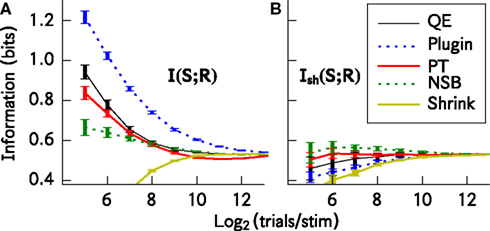
Figure 1. Comparison of the performance of different bias correction methods. The methods were applied to spike trains of eight simulated somatosensory cortical neurons (see text). The information estimates I(S; R) and Ish(S; R) are plotted as a function of the available number of trials per stimulus. (A) Mean ± SD/2 (over 50 simulations) of I(S; R). (B) Mean ± SD/2 (over 50 simulations) of Ish(S; R). This calculation is very similar to that in Panzeri et al. (2007
, Figure 3
), which also used realistic simulations of cortical spike trains (the only difference was that for this figure, the simulated population did not contain any correlations). This figure was produced using the Python library for bias corrections described in Section “A Python Library for Information Theoretic Estimates”, and the code to produce it is available at http://code.google.com/p/pyentropy/
.
While the basic plug-in entropy calculation is a straightforward sum of logarithms, the correction methods described above add significant complexity to the required calculations. In QE, the underlying entropy calculations have to be run many times, for PT the Bayesian estimate of the number of stimulus responses involves additional calculations and NSB involves a complicated procedure of many numerical integrations. For large data sets, with the large probability spaces that can often arise from modern physiological techniques, performance can be an issue as these computational methods become increasingly CPU and memory intensive. Since the performance of bias correction procedures depends on the statistics of data under analysis, in each data analysis task it is also important to test the accuracy of information estimation methods on simulated data with statistical properties similar to the actual experimental data of interest (Panzeri et al., 2007
). It is therefore crucial that these methods be implemented as efficiently as possible. An advantage of Python is that one can benefit both from the improved development time due to the simple syntax and interactive environment, as well as a number of well developed methods for optimising the performance critical portions of the code when necessary. There are tools for automatically converting Python to C inline, inserting your own C code within a Python program, writing full C and FORTRAN extension modules or using Cython, which is a variant of the Python language with a similar syntax but that compiles straight to C code.
A Python Library for Information Theoretic Estimates
The study and development of techniques for estimation of information theoretic quantities and associated bias corrections has developed into a field of its own. In order for the results of this work to be useful outside of this small community it must be possible for non-specialists to easily apply these techniques to their data. We have therefore developed a library of tools with the dual purpose of allowing easy application of the most suitable cutting edge bias corrections, while also providing a framework for continued enhancement of existing methods as well as development of new techniques. Although this has been developed for application to investigations of neural coding, the library has been designed to be as general as possible, in the hope that it might also be of use in other areas, and it is publicly available under an open source license
3
. There are similar packages available in other languages, such as the R entropy library
4
and the MATLAB Spike Train Analysis Toolbox
5
, but the authors are not aware of any similar Python package.
At the core of the library are two classes, DiscreteSystem and SortedDiscreteSystem which sample and store the probability distributions associated with a system and contain methods to compute different entropy quantities. DiscreteSystem is the most general and can take arbitrarily ordered input. The class is initialised as s=DiscreteSystem(X, X_dims, Y, Y_dims) where X_dims=(Xn,Xm) and Y_dims=(Yn,Ym) are tuples of values describing the parameters of the X and Y spaces respectively. Xn and Yn are the number of variables in the space, each of which is quantised to take one of Xm or Ym possible values, respectively. In total therefore there are XmXn possible values in the X space and YmYn in the Y space for each trial. X and Y are provided as integer arrays with values in [0, Xm − 1] and [0, Ym − 1] respectively with Xn, Yn rows representing the constituent variables and a column for each trial. It is important the columns match, that is the value of X in a given column corresponds to the same trial as the value of Y in the same column, but there are no further requirements on the format of the input. SortedDiscreteSystem requires the input trials to be grouped in values of the variable Y. This allows much more efficient sampling of the required probability distributions, since the trials for a given Y value can be easily isolated without having to search through the whole data set. This requires the space Y to be a single finite alphabet variable, so it should be decimalised beforehand if necessary. The class is initialised as s = SortedDiscreteSystem(X, X_dims, Ym, Ny) where X, X_dims are as above and Ym is the number of possible values for the single variable Y space. Ny is an array containing the number of trials available for each Y value. For example, Ny[ ] is the number of trials available with Y = , and the corresponding X values are found at X[ : Ny[]]. Both of these classes inherit from a base class BaseSystem which contains the common entropy and information calculations, reducing code duplication and increasing maintainability.
] is the number of trials available with Y = , and the corresponding X values are found at X[ : Ny[]]. Both of these classes inherit from a base class BaseSystem which contains the common entropy and information calculations, reducing code duplication and increasing maintainability.In neural coding applications such as those described previously, Y would be the stimulus space S, while X would be the response space R. Since the stimuli are usually controlled by the experimenter, the results are often available already sorted by stimulus, allowing use of the more efficient SortedDiscreteSystem class. Mutual information is symmetric, I(X; Y) = I(Y; X), so in fact the stimulus and response spaces can be provided in any order, but due to the way the conditional probabilities are sampled it is strongly suggested that the smaller of the two spaces be provided as the Y parameter.
Once initialised as above, entropy quantities can be calculated using the method s.calculate_entropies(method, sampling, calc) where method is one of [‘plugin’,‘pt’,‘qe’,‘nsb’] and selects the bias correction technique to use, sampling is one of [‘naive’,‘beta:x’,’shrink’] which selects the method for estimating the probability distributions and calc is a list containing a number of entropies to calculate. The entropies available are [‘HX’,‘HY’,‘HXY’,‘SiHXi’,‘HiX’,‘HiXY’,‘HshXY’,‘ChiX’], which in the case where, as described above, the space X corresponds to the response space R and Y to the stimulus space S, denote respectively H(R), H(S), H(R|S), , Hind(R), Hind(R|S), Hsh(R|S) and χ(R). χ(R) is a quantity needed for the information breakdown of (Pola et al., 2003
) and is reported in Eq. 25 therein. This function will first decimalise the X and Y spaces, if required (if n > 1) which involves converting the length-n base-m words representing the values for each space to a single decimal integer value in [0, mn − 1]. The probabilities required for the requested output entropies are then computed using the sampling method specified. “naive” represents the standard histogram bin counting method which is usually used. The add-constant estimator (Schürmann and Grassberger, 1996
) is implemented through the “beta:x”method. The β parameter is provided after the colon in the option, so “beta:.1” would use the add-constant estimator with β = 0.01. The “shrink” option selects the James–Stein shrinkage estimator (Hausser and Strimmer, 2008
). All the entropy estimates are currently implemented in pure Python, except for the NSB estimator. This is implemented using existing publicly available optimised codes
6
. We have not yet implemented a direct link to the NSB codes, but instead write the data for analysis to a file, for processing by the standalone external program before reading back results from a file. Python’s heritage as a scripting language makes this process of reading and writing formatted files and programmatically calling an external program from the code very easy. The functions s.I() and s.Ish() can be used to obtain the mutual information estimate and shuffled mutual information estimate respectively, provided the required entropies have been computed. Similarly s.pola_decomp() will return the computed values for the decomposition of the mutual information presented in Pola et al. (2003)
, again provided the required entropies were computed.
.1” would use the add-constant estimator with β = 0.01. The “shrink” option selects the James–Stein shrinkage estimator (Hausser and Strimmer, 2008
). All the entropy estimates are currently implemented in pure Python, except for the NSB estimator. This is implemented using existing publicly available optimised codes
6
. We have not yet implemented a direct link to the NSB codes, but instead write the data for analysis to a file, for processing by the standalone external program before reading back results from a file. Python’s heritage as a scripting language makes this process of reading and writing formatted files and programmatically calling an external program from the code very easy. The functions s.I() and s.Ish() can be used to obtain the mutual information estimate and shuffled mutual information estimate respectively, provided the required entropies have been computed. Similarly s.pola_decomp() will return the computed values for the decomposition of the mutual information presented in Pola et al. (2003)
, again provided the required entropies were computed.The module has been designed to be as flexible as possible, allowing comparison of the different methods at every stage. For example, the DiscreteSystem instance contains the sampled probability distributions, so it is possible to compare the different probability estimation methods directly. It is easy to add additional entropic quantities or new functions of them to the class. The code is documented through use of Python docstrings, which are embedded in the source and accessible through the interactive interpreter. Having the code documented in this way makes it easier for others to understand and contribute to.
There are several properties of Python that make it well suited to this application. Many loops can be vectorised into a single operation acting on arrays which is implemented through the NumPy interface to a highly efficient linear algebra library (ATLAS). When taking slices (extracting a single row or column) of a NumPy array, for example when determining the independent probabilities of the X variables, a new view is created, but points to the same original data. In contrast, in MATLAB, taking such a slice always results in the extracted row being copied in memory to a new array object. As discussed, the object-oriented nature of Python allows code reuse through inheritance. To give an example of the performance of the Pyentropy library, for the preparation of the data for the Plugin, PT and QE methods in Figure 1
, the time taken using the Pyentropy library on a 2.4GHz Core 2 Duo laptop was 439 s. This includes data simulation for 50 trials at each sample size. The same task, using similar MATLAB code on an equivalent laptop was 987 s. There is also work in progress to extend the Pyentropy code with a more direct calculation of the core estimates in Cython. Cython is a language for writing C extensions to Python, and it shares a very similar syntax. This provides an easy way to quickly develop fast C modules to speed up the execution of Python code.
Correlations and Maximum Entropy Models
Simultaneous recordings of the activity of individual neurons placed within local networks in the central nervous system show that most pairs of neurons are weakly correlated: the probability of observing simultaneous spiking is typically sightly – but significantly – different to the product of the probability of observing the individual spikes (Averbeck et al., 2006
; Mastronarde, 1983
). These correlations are hypothesized by many investigators to be a fundamental part of the neural population code; they may contribute, for example, by tagging the occurrence of particular salient stimulus combinations (Gray et al., 1989
), or by constraining the number of possible network states so that the network may perform error corrections (Schneidman et al., 2006
). Whatever the role of correlated firing, an observer of neural activity (either a data analyst or a downstream neural system) trying to assess the importance of correlated activity has to face a hard problem: correlations are difficult to sample because they are described by a number of parameters that increases exponentially with the number of cells considered. Therefore, it is important to establish whether it is possible to describe all correlations between neurons with a small number of parameters that preserve all the relevant features of the joint distribution of simultaneous responses. One way to find compact representations of the correlation structure of response probability can be obtained by using the technique of maximum entropy (Montemurro et al., 2007b
; Schneidman et al., 2003
; Tang et al., 2008
; Victor, 2006
), as follows.
The question addressed by maximum entropy models is how well we can describe all interactions between all variables in terms of subsets of interactions between up to K variables only, or whether and to what degree higher order interactions are present and important. The maximum entropy technique compares the measured response probability to one that takes into account all the observed interactions of up to K elements but does not impose any additional structure on the data. Measuring all interactions of up to K variables means measuring all the marginal response probabilities involving up to K variables. Therefore any probability matching the observed interactions of up to K elements must obey (apart from the usual non negativity and normalization constraints) the following linear constraints. Here we consider a response vector r = {r1,…, rL} of dimension L, with each variable ri taking values from a finite alphabet A containing m elements.
Each line above denotes a family of constraints on a model distribution PK(r) enforcing equality of the marginal values of a given order to those of the true distribution P(r). These marginals are denoted by η with subscript indices representing the variables involved in the marginal and superscript indices the corresponding values. The ath order constraint applies for all unique combinations of a variables, and every permutation of possible values that those variables can take. Thus the ath line above represents constraints, the product of permutations of a values with choices of a variables.
The probability distribution PK(r) with maximum entropy among those satisfying the above constraints is the one that does not impose the presence of any additional higher order correlations or interactions between the variables. To choose a distribution with lower entropy would correspond to the assumption of some additional structure that we do not know; to choose one with a higher entropy would necessarily violate the constraints that we wish to enforce.
Following Amari (2001)
; Cover and Thomas (2006)
it can be shown that there is a unique solution to the constrained maximum entropy problem, which can be written in the following exponential form:
The set of indices i1,…,ia label the subsets of a variables among the total L considered. The set of indices ri1,...,ria labels a specific set of values of these variables. The first term in the sum is a finite alphabet Kronecker delta function which takes the value 1 when the variables of the argument specified by the subscript indices take the values specified by the superscript indices, and 0 otherwise. As with the marginal constraints, the second sum for each order is over all unique combinations of a variables and all permutations of a values that those variables can take; there are summands, and the same number of distinct θ coefficients of that order.
In order to compute the maximum entropy distribution PK(r; θ) compatible with all the known interactions up to K-th order, we need to find the θ coefficients with up to K indices to construct the solution above. These can be determined from the knowledge of the experimental η marginal probabilities of up to K elements through a set of algebraic equations, as detailed in the following section.
Previous applications of the maximum entropy approach have included temporal sequences of spiking activity, or multi-unit spiking activity across a population, both of which are binary. This simplifies the calculation of the maximum entropy solutions. The extension to a finite alphabet probability space is a significant one, since it greatly increases the scope of possible applications for the method. For example, if larger time bins are used, there will sometimes be more than one spike occurring in each bin. At the moment these values are generally binarized, but using the finite alphabet method allows use of extended time bins, while keeping the effect of all spikes. It can therefore be used to investigate the effect of bursting. Similarly, the finite alphabet extension means the method can be applied to other data, such as LFPs (Belitski et al., 2008
) or fMRI, which are inherently continuous but may be meaningfully quantised into a finite alphabet. It also allows investigation of the reverse problem, neural encoding, where one studies the properties of the stimulus, given that a response (such as a spike) as occurred.
In the following, we describe an implementation of the finite-alphabet maximum entropy computation using Python. In analogy to Schneidman et al. (2003)
, we apply the maximum entropy calculation to P(r). However, the same procedure could be in principle applied to P(r|s).
An Algorithm for Finite-Alphabet Maximum Entropy Solutions
The key concept in the algorithm we use to obtain the maximum entropy solution is the idea of identifying a specific probability distribution using different coordinate systems. The most obvious way of characterising a discrete probability distribution is by specifying the full list of probabilities for each element of the space. For example, if we have a finite alphabet response vector r = {r1,…,rL} as above, then there are mL possible values for r and so the probability distribution P(r) can be characterised by mL − 1 probability values, since one degree of freedom is removed by the normalisation constraint. These are called the p-coordinates. An alternative way of uniquely determining a probability distribution is by listing the marginal probability values. As mentioned in the previous section, there are marginals containing of order k, so the collection of all marginals has elements. This way of describing the probability is called the η-coordinates. For the final characterisation of a probability distribution, we consider the form suggested by Eq. 10. Taking K = L, PK(r) = P(r) and Eq. 10 shows that any probability can be computed from the set of coefficients, θ. Again there are coefficients of each order k. θ0 is fixed by the normalisation condition, so again we have mL − 1 numbers that uniquely identify the probability distribution. Expressing a probability distribution in this way is also known as the log-linear form, and the coefficients, θ are called the log-linear effects. Here we refer to them as the θ-coordinates.
A given probability distribution is represented in any of these coordinate systems by a vector of values. In the following p denotes a vector describing a probability distribution in the p-coordinates, η denotes a vector of η-coordinate values and θ a vector of θ-coordinates. The p vector is ordered so that the value of the vector at a given index represents the probability of the underlying state which, when interpreted as a length L base m word, has the decimal value of the index. This ordering was chosen since it is easy to convert between state values and vector indices using existing change of basis functions. The vector η = (η1, η2,…,ηL) where ηi is the set of all marginals of order i and similarly θ = (θ1, θ2,…,θL). The ordering of the vector within the subsets of different orders is arbitrary, however it is important that the subsets θi and ηi share the same ordering for each i.
These notions are rigorously developed in Amari (2001)
using the framework of information geometry, in which the set of probability distributions on a given vector space are treated as a manifold, and the properties of the coordinate systems described above are formalised.
Coordinate Transformations
An important step in the numerical method for obtaining the maximum entropy solution is the implementation of the transformations between the different coordinate systems described above for representing a probability distribution.
η–p transforms. The key transformation is that from p-coordinates to η-coordinates. This is a linear transformation which performs the summation of relevant probabilities for calculating the marginal. With the coordinates arranged in vectors, as described above, it can be expressed as
where A is a square matrix containing binary values. Each row of A contains a 1 in the column for each p coordinate that contributes to that marginal. The inverse transformation, p coordinates from η coordinates is simply
The matrix A is invertible since it is square and all its constituent rows are linearly independent.
θ–p transforms. For the θ–p transformations, first notice from Eq. 10 that in vector form p = eθ0 + AT0. This is because, for a given probability, the θ terms required are those corresponding to the non-zero elements of that specific state vector. Similarly, for a given probability, that probability will appear in the sum for the marginals corresponding to the same non-zero elements of the state vector. The marginals that a given probability appears in are given by the columns of the matrix A, so provided the θ vector is ordered in the same way as the η vector, the sum of θ terms required in the exponential of Eq. 10 for each probability is given by ATθ. By evaluating Eq. 10 for the zero state vector we see that the constant factor in the log-linear model, eθ0, is in fact p0. From P = p0eATθ, it is trivial to obtain the following transformation from p coordinates to θ coordinates.
The other direction is slightly more complicated, since for a closed expression for p we must compute p0 from the theta vector. The normalisation condition requires that ∑p + p0 = 1, since the vector p does not include the p0 value. Substituting the expression above gives yielding
Numerical Optimisation
The advantages of the different coordinate systems described above are that they allow us to easily represent our constraints on the maximum entropy solution. From Eq. 9 fixing interactions up to order K to those of the measured distribution corresponds to setting the low order η-coordinates of the maximum entropy solution equal to those of the measured distribution. From Eq. 10 the maximum entropy constraint is enforced by setting the high order components of the θ-coordinates to zero. By enforcing these constraints simultaneously, we obtain a set of N simultaneous equations in N unknowns, where is the number of coordinates up to order k. Again m is the size of the finite alphabet.
In the following ηk represents the N low order (up to order k) marginals of the sampled distribution. θk, θk, represent the low and high order theta coordinates of the maximum entropy distribution. denotes the coordinate transformation from θ to p coordinates from Eq. 14 and denotes the coordinate transformation in Eq. 11 but with only the low order marginals returned. Setting the high order theta’s, θk+, to zero ensures that there are no higher order interactions. It is then possible to find the low order theta’s that produce the same low order marginals as the sampled distribution, ηk. These low order theta’s, θk, completely characterise the maximum entropy distribution. In vector form the equations are:
Once the θk are determined by numerically solving the equation above, one can convert back to p-coordinates to obtain the corresponding maximum entropy distribution and calculate its entropy.
Python Implementation
Initially the method described above was implemented in MATLAB. Later, the same algorithm was converted to Python with NumPy and SciPy. This was both because we were having performance issues with MATLAB in the finite alphabet case, and partly as a way to evaluate Python as a platform for our work. This gives the opportunity to make comparisons between the two systems. However, as well as moving the code to Python, we continued to develop and improve the algorithms, making it difficult to provide rigorous performance comparisons between the two systems. Instead we hope to provide an overview of our experiences and impressions of using Python in an ongoing research project.
A major difference in the code between the two systems is the structure of the program. In MATLAB the notion of the global workspace was exploited. Here a setup script is used to define the coordinate transformation functions in the global workspace, from where they can be easily called by other scripts or used to interactively investigate data. In Python, an object-oriented approach was taken featuring two main classes. The first of these, AmariSolve, contains the parameters related to the underlying probability distribution, the required coordinate transformations and the code for performing the numerical solution. This is initialised with two parameters, the number of variables and the finite alphabet of each variable, since this is the only information required to implement the solution. The second class, AmariSystem, contains the data related to a specific system being studied, and contains the sampled probability distributions, calculated maximum entropy distributions and associated entropies. In this way the data independent analysis code is separated from the system specific code and data – the idea being that a single AmariSolve instance can be used on different data sets, providing the dimensions of the probability space are the same. It was found this approach gave much more flexibility than the global workspace, which could be confusing to manage during development, for example by requiring a full copy of the setup script to be maintained for every change to the algorithm investigated.
A key step in the implementation of the algorithm is the generation of the matrix A which provides the transformation between probabilities (p-coordinates) and marginals (η-coordinates). A recursive function is used in a loop over each order, to compute the elements of A row by row. The code implements the longhand approach used for manual calculation of smaller matrices. The idea is that each marginal is the sum over all variables not fixed by the specification of the marginal. For each order a vector called terms is created which contains all base m words of length L − o, where o is the order being considered. Then for each marginal, if columns of the appropriate value are inserted into the appropriate position in the terms array, the result contains a row for each probability state included in that marginal. These are converted to decimal, which directly gives the index in the probability vector, and the corresponding columns in A are set to 1. To cover the different marginals, first the alphabet value and then the position is looped over. For orders higher than one, this process is recursive, so the first alphabet value is looped over, then within that the first position, then within that the second alphabet, then the second position and so on. This transformation matrix can be very large since its dimensions are the dimensions of the full probability space. However, it is highly sparse in structure, so in both implementations the provided sparse array construct was used to reduce the amount of memory required. In SciPy, the sparse array module is very flexible, providing a number of formats and datatypes. The advantage of this was that the binary matrix A could be stored as a sparse array of 8-bit integers in SciPy, which provided a factor of eight memory saving over the 64-bit double which is the only type the MATLAB sparse matrix supports. Equations 12 and 13 show that some coordinate transformations require inversion of the matrix A. Although this is not required directly for the computation of the maximum entropies, it was frequently useful while investigating properties of the system and of the different maximum entropy solutions. SciPy offers a very flexible direct interface to the UMFPACK
7
library of sparse solvers (Davis, 2004
), that allowed us to easily pre-factor the matrix and store the results allowing rapid calculation of the coordinate transforms when needed.
The numerical optimisation step is very similar in both implementations, using the fsolve function of the respective system. In MATLAB a Gauss–Newton method was used, while in SciPy fsolve is a wrapper around the MINPACK (Moré et al., 1999
) hybrd algorithm which implements a modification of the Powell hybrid method. Both of these methods performed similarly. The function that the optimiser runs is the same in both implementations and this is a direct implementation of the left hand side of Eq. 15; the Python version is shown below. Here Asmall is a subset of the transformation matrix A containing only the rows required and Bsmall is the transpose of this. Asmall is extracted from A using the slice operator, for example in Python, Asmall = A[:l, :]. Python again provides a significant advantage here in terms of memory used. In MATLAB, any such slice results in a copy of the data. However, with NumPy, the slice results in a view of the original data. Similarly, in NumPy the transpose is also a view, with a different starting point and striding, but the same data buffer as the original array. In MATLAB the transpose operation also produces a copy.
def solvefunc(self, theta_un, Asmall, Bsmall, eta_sampled):
b = np.exp(Bsmall.matvec(theta_un))
y = eta_sampled(Asmall.matvec(b)/(b.sum() + 1) )
return y
As the method was developed and applied to increasing large probability spaces, it became clear that the limiting factor for these more challenging parameter sets was the memory usage rather than the computation time. The Python implementation was therefore optimised to reduce the memory usage.
This enhancement was simplified by using the object-oriented features of Python. New classes were created which inherited from AmariSolve and AmariSystem described above. It was then possible to change only the required functions, for example the matrix generation routine, to stop at the required row. This minimised the other changes and duplication of code. Also, developing in this way meant very few changes were required to the analysis scripts to take advantage of this change – in most cases a simple substitution of the class name at the top of the script was enough to use the new method. One of the memory optimisations was to produce the matrix A in smaller blocks, writing the rows and columns of the non-zero elements directly to files on disk to reduce memory overhead. Once this procedure was completed a sparse matrix in coordinate (COO) format could be generated directly from these files, and then converted to compressed sparse column (CSC) format for efficient matrix-vector multiplication. This is another example of where good results were obtained by using low level features that would not have been available in MATLAB.
As an example of the relative performance of Python and MATLAB, maximum entropy solutions of up to second order were computed for a system with n = 4, m = 9 (four variables each taking 1 of 9 values). The MATLAB code took 17 s with a peak resident memory usage of 340 MB and the Python code took 12 s with a peak resident memory usage of 110 MB. These results are typical of our experience across a range of parameter values. The numerical optimisation routine took almost exactly the same time in both systems, with the difference being due to the improved performance of the sampling of the probability distributions in Python. This is likely to be due to the reduced amount of data copying needed with NumPy when using slicing and other array operations.
In conclusion, for the development of this technique the use of Python with NumPy and SciPy libraries as an alternative to MATLAB was highly successful. The computational speed was very similar, but using NumPy allowed us to reduce the memory requirement by around two-thirds. This is important, because as described above, memory usage was the limiting factor restricting the size of the probability space over which the analysis could be performed. As well as the vectors representing the actual probability distribution, the sparse matrix A must be calculated and held in memory. The ability to use an 8-bit integer for this binary matrix with Python provided a factor of 8 memory saving over the MATLAB equivalent. More significantly, the algorithm requires extraction of the submatrix of up to the relevant order, and the transpose of that, which in MATLAB consists of copies (meaning for each order the data is copied in memory three times, once for the full matrix A, once for the extracted Asmall for the given order, and once for the transpose thereof, Bsmall). As an example, this meant that on a workstation with 2 GB of RAM the largest binary probability space that could be analysed up to order 3 was 12 variables for the MATLAB implementation, but 18 variables for the Python version. It is also worth noting that, while being similar to MATLAB, the Python language is a great pleasure to work with.
Example of application to thalamic neural recordings
To illustrate the application of maximum entropy techniques, here we compute maximum entropy models from a neuron in the ventro posterior medial nucleus (VPm), which is the principal whisker-related relay nucleus in the rat thalamus. Using extracellular microelectrodes, we recorded the responses of single VPm units in anaesthetised rats whose whiskers were mechanically stimulated with a piezoelectric wafer driven by a low-pass filtered white noise (see Montemurro et al., 2007a
, for details). We used two types of white noise stimulation. The first sequence was identical on every trial (repeated stimulus); the second was independently generated on every trial (non-repeated stimulus). Figure 2
B shows a raster plot of the spikes fired by a single neuron in response to 70 repetitions of the stimulus in Figure 2
A. As previously reported (Montemurro et al., 2007a
; Petersen et al., 2008
), VPm responses to white noise were highly repeatable and temporally precise. An information theoretic analysis of these data revealed that these neurons convey information at sub-ms temporal precision (Montemurro et al., 2007a
) and that there are correlations between the times of individual spikes. One source of correlation came from the refractoriness of neurons, and another source of correlation came from their tendency to fire spikes in bursts (Montemurro et al., 2007a
). An important question is whether these correlations between the times of spikes emitted by the same neuron have a significant impact on the information and entropy of the neural spike train, and if these correlations can be described by simple pairwise models or if they rather need a complex, high order characterization. Here we will address these questions by using maximum entropy models which, as explained above, provide a natural framework to study the impact of different orders of correlation to spike train entropy and information. Previous studies employing maximum entropy have focussed mainly on correlations across a population of neurons (Schneidman et al., 2006
; Shlens et al., 2006
). Here, we extend this study to focus on correlations in time between spikes of a single neuron. This is interesting because finding a compact maximum entropy representation of within cell correlations is an important step towards understanding spike timing codes and representing them efficiently (Nirenberg and Victor, 2007
; Tang et al., 2008
).
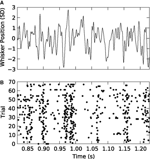
Figure 2. Responses of a VPm neuron to white noise vibrissa stimulation. (A) Vibrissa position as a function of time in units of stimulus SD (1 SD = 70 µm). (B) Spikes fired by the neuron in response to 70 repetitions of the stimulus shown in (A).
We discretized the time into small bins of size Δt = 4 ms and quantified the response of the considered VPm neuron as a binary sequence of 1’s and 0’s (spikes or silence in that bin respectively), characterising the neural response r as non-overlapping binary words of length L extracted from this signal. We then considered the probability of response P(r) in response to all patterns of whisker stimulation obtained from the non-repeated white noise sequences, and we compared its entropy to that of the maximum entropy probability PK(r) at level K (K = 1,…,3) and to the entropy of the true distribution. Results are reported in Figure 3
. We found that the lowest order model (K = 1, which considers spikes in each bin as independent from each other) provides an entropy very close to that carried by higher order probability models. The difference between lower and higher order entropies becomes proportionally larger as the length L of the binary word increases. However, differences remain small: for L = 14, the difference between the independent-model, K = 1 entropy and the true one remain within 3%. This suggests that the spike train could be quantitatively well described even by a simple model that ignores correlations between spikes at different time bins. It should be noted that in the Python implementation of this calculation, the limit on the maximum number of time bins L and the order K that could be analysed was set by the number of trials available and the effectiveness of the sampling bias corrections implemented, whereas in the corresponding MATLAB implementation the limit was reached when the available memory was consumed. For a binary system as described here that limit was L = 12, K = 2 on our workstation. This highlights the advantages of Python for these implementations.
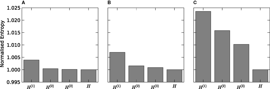
Figure 3. Response entropy of a VPm neuron to white noise vibrassa stimulation. The full response entropy [H(R) denoted H in the figure] is shown together with that of maximum entropy models preserving first [H(1)], first and second [H(2)] and up to third order [H(3)] marginal densities. The response is treated as non-overlapping words of length 6 (panel A), 10 (panel B) and 14 (panel C) bins, with each bin of 4 ms duration.
It should be noted that while we are applying the analysis here to data from a single cell, the computational challenge is determined solely by the dimension of the underlying probability space. In this case, the largest underlying probability space considered has a dimension of 214 which is computationally equivalent to the case of the binary response of 14 simultaneously recorded neurons.
There is a growing trend in neuroscience towards the development and use of collaborative computing services. These are multi-user systems, accessed over the internet which provide computational resources while facilitating interaction between users. This is a natural evolution for the field, as rapid advances in physiological techniques of many kinds result in data sets of increasing size and with an associated proliferation of analysis tools of increasing complexity. The idea is to provide an environment to foster collaboration, especially between experimentalists and theoreticians, by providing databases of experimental results, and online analytical tools for application to those data.
The field of bioinformatics has pioneered the development of such systems, which are now well established and playing an important role. However, implementing such systems for neuroscience presents some challenges not faced by the bioinformatics community. The greatest of these is the volume and variety of experimental data. While traditional bioinformatics services tend to process data as strings – which is partly why the Perl programming language still underpins much bioinformatics analysis – in neuroscience we deal with large sets of binary data in a variety of different formats. This presents difficulties for the decentralised model of separately provided and hosted services that has become popular in the bioinformatics community. This data requires significant contextual detail, or metadata, to be useful and is large enough to make the sharing of terabytes of data between labs a significant issue. It therefore seems that neuroscience requires a stronger organisational structure for these systems, to facilitate easier interoperability of data and provide security and access control.
The adoption of Python is highly advantageous in this context. The Python language is flexible, extensible and runs on a wide range of platforms. It also has the fast array mathematics crucial for neuroscience work, which are not available in languages such as Perl, which have been traditionally used for bioinformatics services. Like Perl though, it is a dynamic interpreted language, which simplifies the deployment of code on distributed systems. It has a similar syntax to MATLAB, the established standard in the field, and although there are no automated tools, translating code and algorithms from one to the other is relatively straightforward. Unfortunately it is difficult to use MATLAB to provide these kinds of multi-user services due to licensing restrictions. We are working on adapting our information theoretic techniques for use in systems of this type, and this was one of the factors that influenced our decision to investigate Python.
The Code, Analysis, Repository and Modelling for e-Neuroscience (CARMEN)
8
project is a consortium effort to create a virtual laboratory for neurophysiology (Gibson et al., 2008
), and is one example of project attempting to provide a centralised organisational structure for collaborative computing in neuroscience, as discussed above. CARMEN is an e-Science Pilot Project funded by the Engineering and Physical Sciences Research Council (UK) and involves investigators from 11 UK universities.
The goals of the CARMEN project are to create a decentralised computing resource used by experimentalists and theoreticians alike; a repository for both experimental data and analysis code that can be made available to all users of the system. We are working to provide our Python-based information theoretic algorithms as “services” on the CARMEN system. Providing such packaged services as modules that can be used in easy to construct “workflows” has many advantages. It allows easy comparison of different analytical techniques on the same dataset, as well as allowing application of a given technique to a number of different datasets that might otherwise be hard to obtain or convert to a suitable format. It allows application of the techniques of information theory by experimentalists and others who may otherwise lack the mathematical background, programming skills or inclination to implement such techniques by hand from the literature. It should also allow better reproducibility of published results, as well as providing a substantial computational resource allowing calculations that could be too time consuming for a user to perform on a desktop computer.
Python Web Services
A “web service” is “a software system designed to support interoperable machine-to-machine interaction over a network”
9
. Web services are well suited to collaborative computing services, and they have been proven as a successful model for e-Science through their use in the bioinformatics community. They are also used as the foundation of the analysis code in the CARMEN project described above. Web services are operating system, location and language neutral. This is exploited in CARMEN to allow dynamic deployment of services to different computational nodes, and also simplifies the use and integration of analysis code written in a range of languages.
There are a number of standards governing the behaviour of web services, largely provided by the World Wide Web Consortium (W3C), which are required to allow them to interact. The fact that these standards are vendor neutral has enabled them to gain traction where previous attempts to provide interoperable services has failed. Simple Object Access Protocol (SOAP)
10
is a standard XML based messaging format used to pass data and parameters to an analysis service, and then receive the results back. All clients and web services are capable of passing and decoding SOAP messages. The other pivotal standard is that of the Web Services Description Language (WSDL)
11
, an XML document for the description of a web service; that is the method calls it provides, the arguments they require and the results they return. The WSDL that represents a web service is sufficiently informative to allow automatic generation of clients capable of binding to the service.
As part of our work we are making the information theoretic techniques that we are developing available as web services, for use in CARMEN and similar systems. Python greatly eases this process. We can create a Python-based service for a specific information theoretic task simply by importing our information theoretic library and calling the appropriate function with the appropriate arguments. This reduces code repetition, and the flexibility and simplicity of the Python module system makes the process easy to manage. For example, if the algorithmic code was actually included in the service programs, this would exist in every service performing an information theoretic calculation with a copy on every node to which the service had been deployed. By having a library with a consistent API, this can be updated in a single place on each computational node without having to change any of the existing services.
Once there is a Python script to perform the required task, it is necessary to “wrap” it to create a web service. There are a number of toolkits to do this including the Python native Zolera SOAP Infrastructure (ZSI) and SOAPpy. However, the method we have been using is InstantSOAP
12
a generic toolkit capable of exposing legacy applications as web services. Initially, we have created Python scripts that run as command line applications. This is straightforward since Python includes an excellent tool for easily parsing command line options. InstantSOAP provides a native command line processor to wrap any command line application into a web service through the creation of a single XML file. Work is currently in progress to extend InstantSOAP to natively support Python services, allowing direct deployment of a Python function as a web service, without requiring the developer to understand the web services stack, a significant barrier to entry in developing web services in any language. Python’s licensing model is also important in the deployment of distributed services; MATLAB suffers from licensing restrictions for collaborative deployment. This makes it harder both to provide open services to a large number of users and to employ the dynamic deployment architecture through which code may run on a number of computational nodes. For example, whilst CARMEN is capable of providing MATLAB web services, it is through compiled MATLAB scripts, supported by the MATLAB runtime environment, and has no native interface to MATLAB per se, adding additional complexity to the procedure of creating, deploying and managing web services. There are also a number of ongoing technical challenges related to running the compiled MATLAB binaries within the web service environment.
In modern neuroscience a growing challenge is handling and interpreting increasingly large volumes of physiological data of many different types. To face this challenge computational techniques are becoming more and more important. We have described information theory, which is one such technique that is particularly suited to the challenges posed by neurophysiological datasets, and can provide valuable insights into neural coding and the function of the nervous system.
Information theory provides a natural framework to study communication in most systems, and the brain is no exception. An obstacle to a wider spread of its use among sensory neurophysiology laboratories has been the technical difficulties associated with its calculation (mostly the problem of bias corrections) and the lack of well defined, cross-platform packages that can handle generic datasets. The work presented in this paper is an attempt to address this limitation and provide the neuroscience community with open source packages that allow unbiased calculation of information from various types of neural data, from spikes to field potentials. The use of Python helps to develop flexible tools that can easily be applied or extended (because of the flexibility of the Python language) to handle different types of neurophysiological signals (because of the ability to manage memory efficiently) and to different data formats (because of the ability of Python to easily read a variety of data formats commonly used in neuroscience).
We have also described a current area of intensive research on neural coding; namely a new implementation for computing solutions of maximum entropy given marginal constraints. Although the example presented in Figure 3
was on a binary data space, the ability of the code to support finite alphabet probability spaces is significant and allows the application of the maximum entropy technique to a wide range of new areas. In our own experience with simulated data (results not shown here, but partly reported in Lüdtke et al., 2009
), using the Python implementation described here we were able to solve maximum entropy solutions of order 2 on spaces of up to 7 variables quantised to 9 levels (a probability space with dimension ∼4.7 m) on a well-equipped workstation in a reasonable amount of time (∼1 day). This was a dramatic improvement over what we were initially able to achieve with the MATLAB version of code; indeed the MATLAB version would have been unable to solve for a system of that size due to memory limitations. Other potential finite alphabet applications include analysis of quantised naturally continuous signals, such as LFP or fMRI as well as opening the possibility of studying the interactions between the stimulus features encoded by spiking responses, where instead of response given stimulus we consider the properties of the stimulus given a response.
Looking to the future of inter-disciplinary science, we have considered the possibilities offered by collaborative computing services based on grid or cloud architectures. While such systems have been developed for use in other areas, neuroscience poses some unique challenges. We have outlined our work as part of the CARMEN project, which hopes to address these challenges and provide a valuable service for storage, processing and analysis of electrophysiological data. We are developing information theoretic analysis tools as web services, which will make them available to greater range of practitioners, and hopefully increase their use within the neuroscience community.
The development of analysis tools like the ones discussed here has potentially significant implications for the refinement, reduction and replacement (3R) of animals in research. In our specific case, the opportunity to easily run information analysis on a number of different existing datasets (which as discussed, is facilitated by Python) maximizes the probability of obtaining new insights into neural codes without the need to sacrifice new animals. The free availability of advanced routines for calculation of bias-corrected information estimates offers neurophysiological laboratories the possibility of reliably computing information from a smaller number of trials, thereby maximizing the potential to record from multiple sites in the same animal and thus reducing the total number of animals needed for statistical significance. The ability of the code to adapt to the different types of neural signals that can simultaneously be extracted from the extracellular signal also increases the amount of information that can be obtained without increasing the invasiveness of the recording procedures.
We have found significant advantages to using Python for all of the work described above. As discussed, we have found it well suited both to reimplementing existing techniques for exposure to a wider audience, as open-source packages and hosted computational services, and to the research and development of new techniques and algorithms. Together with the excellent interactive environment IPython
13
, it provides much of the power available from low level C coding with a numerical library, but with greatly reduced complexity and development time. For example, a major advantage for our maximum entropy application was the way we were able to fine tune the use of the sparse matrix structures. The interactive nature, familiar to users of MATLAB, is crucial to aid research, both in terms of investigation of data as well as development of algorithms. Compared to MATLAB, we have seen performance increases in moving our code to Python, particularly related to memory management in the case of our more demanding algorithms. In addition, increased productivity and code manageability, for example from the ability to use object-oriented programming techniques, speed development and ease collaboration with other researchers.
We have experienced few problems with migrating our code from MATLAB. We have been able to easily access existing data stored in .MAT files and also to smoothly translate code. It is even possible to call MATLAB from Python, through the mlabwrap module
14
, which we have used to run existing MATLAB code provided by colleagues for preprocessing data. Initially the required packages were difficult to install, requiring compilation from source of a range of packages with complicated dependencies. Actually getting the software installed was therefore the greatest challenge when we began using Python. However, since then, the community has done a lot of work in improving this process, and there are now regular binary releases of all the important components, as well as a number of projects that distribute a complete scientific tool chain with all required components through a common installer
15
. Another challenge was adapting to the pass by reference semantics of Python rather than the pass by value style of MATLAB, as well as adapting to 0 based indexing. However, once these mental adjustments had been made we found ourselves more productive with Python than we were with MATLAB. Other disadvantages of Python are that the documentation of the included functions, while still available interactively, is not as comprehensive as that provided with MATLAB and the plotting functionality provided by matplotlib, is not quite as easy to use or well developed as the MATLAB version, especially with regard to 3D plotting.
We have been able to easily provide our Python code as web services, for integration into collaborative systems such as CARMEN, without requiring a significant time investment to adjust or tune the code for this purpose. In fact, Python is an excellent fit for projects such as CARMEN. It provides the flexibility of dynamic interpreted languages such as Perl, that have traditionally been used to provide services in systems of this type, while including the fast array mathematics that are crucial for the efficient analysis of neurophysiological data. It is difficult to use MATLAB in systems such as this, due to licensing restrictions which pose problems, both for allowing multiple users to access the service, and for running the service on different nodes in a grid infrastructure. Obviously, with Python being open source, there are no such issues. The benefits of open source extend beyond collaborative computing projects however; there is a compelling open-access argument for avoiding expensive proprietary software in published scientific work.
So far we have only scratched the surface in terms of what is available in the Python ecosystem that could be of benefit for our work. The extensive collection of modules available for Python allow great flexibility, for example making it much easier to develop GUI interfaces and handle a wide variety of data formats. There are also several methods to easily extend Python code with natively compiled C extensions, to increase the performance of critical sections of code, while still allowing the interactive use and rapid development of Python. We are currently focussed on optimising our information theoretic codes through the use of Cython
16
, which we are finding significantly easier to use and less error prone than the MATLAB equivalent (the MEX interface). Another area we are actively investigating in the use of parallelism. In many cases our problems are embarrassingly parallel, for example calculating information theoretic bias-corrected quantities over a number of data sets or computing maximum entropy solutions of different orders and conditional distributions. A number of open source solutions exist for parallel computing with Python, and we are investigating using these features of IPython to easily distribute these types of jobs to available machines.
The Python library for information theoretic estimates described in Section “A Python Library for Information Theoretic Estimates”, including code for producing Figure 1
, can be found at http://code.google.com/p/pyentropy/
. The code for obtaining the finite alphabet maximum entropy solutions can also be found on that page. This code is provided as Supplementary Material on the conditions that (1) the authorship of the software shall be acknowledged, (2) the present article shall be correctly cited in any publication that uses results generated by the software, (3) any publication that uses results generated by our software shall correctly cite the original articles (cited in this paper) which developed any bias correction methods used.
The authors declare that the research was conducted in the absence of any commercial or financial relationships that could be construed as a potential conflict of interest.
This work was supported by the EPSRC “CARMEN” grant and by IIT. We are indebted to C. Magri, R. Senatore, F. Montani, N. Ludtke and M. A. Montemurro for useful discussions on the implementation of entropy methods and for important contributions to the development of the information theoretic algorithms.
- ^ The Mathworks, Inc, Natick, MA. http://www.mathworks.com/
- ^ “Open source is a development method for software that harnesses the power of distributed peer review and transparency of process. The promise of open source is better quality, higher reliability, more flexibility, lower cost, and an end to predatory vendor lock-in.” http://www.opensource.org/
- ^ See http://code.google.com/p/pyentropy/
- ^ See http://www.strimmerlab.org/software/entropy/index.html
- ^ See http://neuroanalysis.org/toolkit/
- ^ From http://nsb-entropy.sourceforge.net/
- ^ http://www.cise.ufl.edu/research/sparse/umfpack/
- ^ http://www.carmen.org.uk/
- ^ http://www.w3.org/TR/ws-gloss/
- ^ http://www.w3.org/TR/soap/
- ^ http://www.w3.org/TR/wsdl
- ^ http://instantsoap.sourceforge.net/
- ^ “An enhanced interactive Python shell and architecture for interactive parallel computing”, http://ipython.scipy.org/ (Perez and Granger, 2007 )
- ^ “A high-level Python to MATLAB bridge”, http://mlabwrap.sourceforge.net/
- ^ See for example http://www.pythonxy.com/ and http://www.enthought.com/products/epd.php
- ^ The Cython language, “C extensions for Python”, http://cython.org/
Gibson, F., Austin, J., Ingram, C., Fletcher, M., Jackson, T., Jessop, M., Knowles, A., Liang, B., Lord, P., Pitsilis, G., Periorellis, P., Simonotto, J., Watson, P., and Smith, L. (2008). The CARMEN Virtual Laboratory: Web-Based Paradigms for Collaboration in Neuroscience. 6th International Meeting on Substrate-Integrated Microelectrodes. Reutlingen, Germany.
Jones, E., Oliphant, T., Peterson, P., et al. (2001). SciPy: Open Source Scientific Tools for Python. URL http://www.scipy.org/
Moré, J., Garbow, B., and Hillstrom, K. (1999). Minpack. URL http://www.netlib.org/minpack
Tang, A., Jackson, D., Hobbs, J., Chen, W., Smith, J. L., Patel, H., Prieto, A., Petrusca, D., Grivich, M. I., Sher, A., Hottowy, P., Dabrowski, W., Litke, A. M., and Beggs, J. M. (2008). A maximum entropy model applied to spatial and temporal correlations from cortical networks in vitro. J. Neurosci. 28, 505–518.