Topographica: building and analyzing map-level simulations from Python, C/C++, MATLAB, NEST, or NEURON components
Institute for Adaptive and Neural Computation, University of Edinburgh, Edinburgh, UK
Many neural regions are arranged into two-dimensional topographic maps, such as the retinotopic maps in mammalian visual cortex. Computational simulations have led to valuable insights about how cortical topography develops and functions, but further progress has been hindered by the lack of appropriate tools. It has been particularly difficult to bridge across levels of detail, because simulators are typically geared to a specific level, while interfacing between simulators has been a major technical challenge. In this paper, we show that the Python-based Topographica simulator makes it straightforward to build systems that cross levels of analysis, as well as providing a common framework for evaluating and comparing models implemented in other simulators. These results rely on the general-purpose abstractions around which Topographica is designed, along with the Python interfaces becoming available for many simulators. In particular, we present a detailed, general-purpose example of how to wrap an external spiking PyNN/NEST simulation as a Topographica component using only a dozen lines of Python code, making it possible to use any of the extensive input presentation, analysis, and plotting tools of Topographica. Additional examples show how to interface easily with models in other types of simulators. Researchers simulating topographic maps externally should consider using Topographica’s analysis tools (such as preference map, receptive field, or tuning curve measurement) to compare results consistently, and for connecting models at different levels. This seamless interoperability will help neuroscientists and computational scientists to work together to understand how neurons in topographic maps organize and operate.
In mammals, much of the cortical surface (and many subcortical structures) can be partitioned into topographic maps (Kaas, 1997
; Van Essen et al., 2001
). These maps contain systematic two-dimensional representations of features relevant to sensory and motor processing, such as retinal position, sound frequency, line orientation, and motion direction (Blasdel, 1992
; Merzenich et al., 1975
; Ohki et al., 2005
; Weliky et al., 1996
; Xu et al., 2007
). Figure 1
shows an example retinotopic and orientation map from the primary visual cortex (V1). Understanding the development and function of topographic maps is crucial for understanding brain function, and will require integrating large-scale experimental imaging results with single-unit studies of the individual neurons and their connections that make up these maps. In principle, computational modeling can help make these links explicit, in order to explain how topographic maps can emerge from the behavior of single neurons.
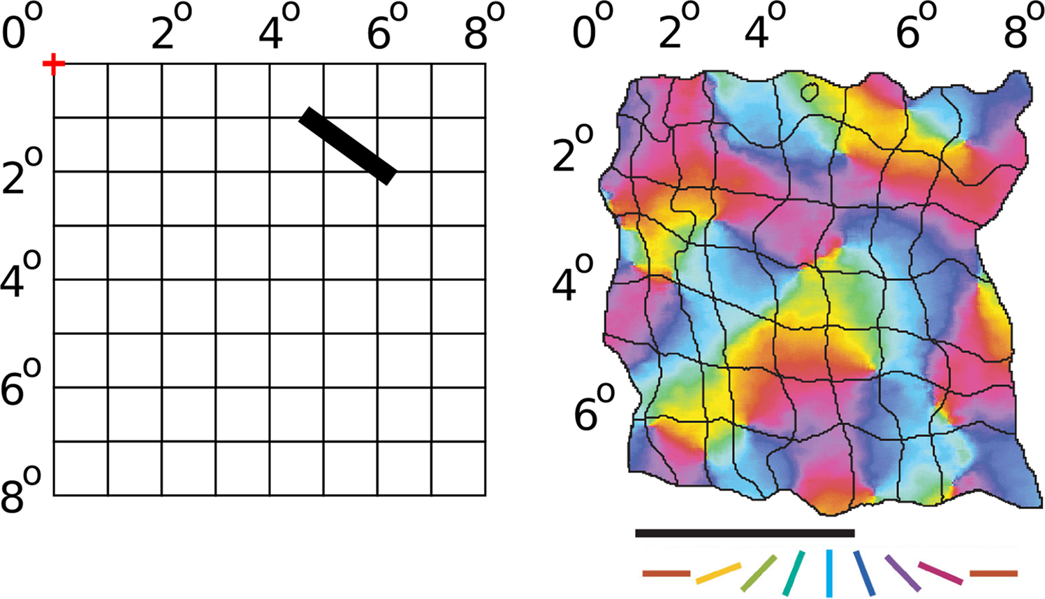
Figure 1. Retinotopic and orientation map in V1. Given a particular fixation point (marked with a red + symbol above), the visual field seen by an animal can be divided into a regular grid, with each square representing a 1° × 1° area of visual space. In cortical area V1 of mammals, neurons are arranged into a retinotopic map, with nearby neurons responding to nearby areas of the retina. As an example, the image on the right shows the retinotopic map on the surface of V1 of a tree shrew for an 8° × 7° area of visual space (adapted from Bosking et al., 2002
with permission; scale bar is 1 mm). A stimulus presented in a particular location in visual space (such as the thick black bar shown) evokes a response centered around the corresponding grid square in V1 (6°, 2°). Which specific neurons respond within that general area, however, depends on the orientation of the stimulus. The V1 map is color coded with the preferred orientation of neurons in each location; e.g. the black bar shown at left will primarily activate neurons colored in purple in the corresponding V1 grid squares. Similar maps could be plotted for this same area showing preference for other visual features, such as motion direction, spatial frequency, color, disparity, and eye preference (depending on species). Other cortical areas are arranged into topographic maps for other sensory modalities, such as touch and audition, and for motor outputs. Topographica is designed to simulate any of these cortical or subcortical areas.
However, existing simulators typically address only a small range of levels of analysis. For instance, NEURON (Hines and Carnevale, 1997
) and GENESIS (Bower and Beeman, 1998
) primarily focus on detailed studies of individual neurons or very small networks of them, rather than enough neurons to form a meaningful topographic map. Topographica (Bednar, 2008
) and NEST (Diesmann and Gewaltig, 2002
) allow much larger scale simulations of simpler neurons, but Topographica provides only limited support for spiking neurons, while NEST provides only limited support for firing-rate neurons (necessary for the largest scale models) or for more detailed individual neuron models, and does not provide a GUI for large-scale visualizations. Combining multiple simulators to bridge between these levels of analysis could provide a complete, biologically grounded explanation of how single-neuron properties lead to large-scale topographic maps. Even for models at the same level, interfacing multiple simulators into a coherent framework can also help provide a uniform means for comparing and evaluating them. However, interconnecting simulators has previously been a significant technical challenge (Cannon et al., 2007
; Djurfeldt and Lansner, 2007
).
This paper describes how the Topographica map-level simulator can be used to achieve important types of interoperability between a very wide range of simulators with surprisingly little coding or development effort. One reason that interoperability is practical in Topographica is that Topographica is implemented in the Python scripting language, and many neural simulators now include Python interfaces. Another reason is that Python is a very high level language, known as a glue language (Ousterhout, 1998
), that makes it easy to connect different interfaces for rapid software development. Even more important, however, is that Topographica is built around a high-level abstraction of the properties of topographic maps, which is relatively simple to adapt to components implemented in any particular simulator yet provides access to a large range of useful tools. Simply put, if a simulation in any other simulator or language contains a large number of neurons (at any level of complexity) arranged into a two-dimensional sheet or array (or a three-dimensional stack of such two-dimensional arrays), then it will be practical to use that simulation or parts of it within Topographica.
In turn, integrating such a simulation into Topographica will be useful if it can make use of analyses that rely primarily on an average (firing rate) activation level for each neuron, particularly if they are based on measuring responses to an input pattern. Many such routines are already implemented in Topographica, such as measuring receptive fields, tuning curves, or feature preference maps of any type, decoding activity values, and 1D, 2D, or 3D plotting of these and other measurements. Other simulators implement some of these functions, but rarely in a fully general form that can be applied to any neural area and any type of input feature. To make the most use of these components, it is helpful if each sheet of neurons in the underlying model can be separated from the others with well-defined interfaces, but even relatively monolithic models can be analyzed if they include at least one sheet of neurons that can accept an external input, and at least one neuron or set of neurons whose firing-rate activity patterns are of interest. Any such model can then be compared and tested against any similar model, using a consistent analysis and visualization framework. Similar considerations apply to using small parts of external models, such as a model retinal or cortical area, as part of a larger hierarchical or network model of a neural system connected in Topographica.
These features make it surprisingly straightforward to use Topographica for simulating and analyzing large-scale, detailed models of topographic maps, using either native or externally implemented components. Topographica is an open source project, and binaries and source code are freely available through the internet at
topographica.org for interfacing to external code on Linux, Microsoft Windows, and Macintosh OS X platforms. In the sections below, we describe the main assumptions and abstractions used by Topographica, provide a detailed example of interfacing to an external spiking simulator, show how to interface to a wide variety of other external systems and simulators, and discuss in more detail which types of models are most suitable for interfacing with Topographica.Models supported natively by Topographica typically consist of a collection of topographic maps in cortical or subcortical regions, such as an auditory or visual processing pathway. Figure 2
shows an example simulation along with various types of analysis and plotting. This simple model consists of four separate populations of neurons, called
Sheets: one sheet of retinal photoreceptors (labeled Retina), a sheet of ON retinal ganglion cell (RGC)/lateral geniculate nucleus (LGN) cells labeled LGNON, a sheet of OFF cells labeled LGNOFF, and a sheet of V1 pyramidal cells labeled V1. Neurons in each sheet are arranged topographically, with similar properties but at different spatial locations.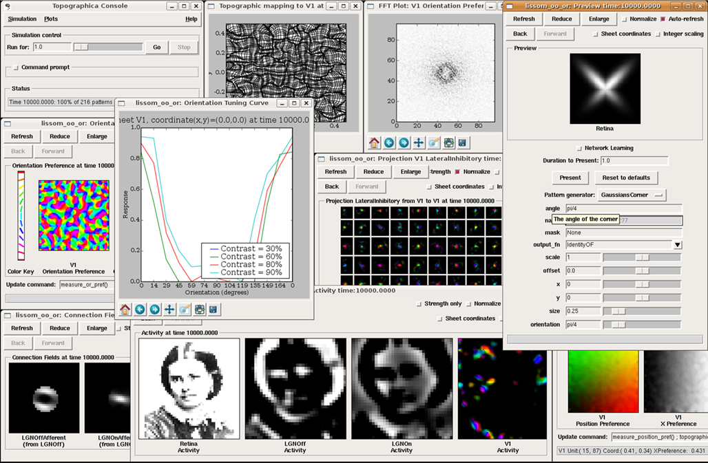
Figure 2. Topographica software screenshot. This image shows a sample session from Topographica version 0.9.3, available freely at
topographica.org. Here the user is studying the behavior of an orientation map in the primary visual cortex (V1), using a model of photoreceptors as the input to the Retina, ON and OFF RGC/LGN cells, and a simple V1 model. The window at the left labeled “Orientation Preference” shows a self-organized orientation map in V1. The window labeled “Activity” shows (from left to right) a sample visual image input to the retina, the ON and OFF channel responses to that input, and (on the right) an orientation-color-coded representation of activity in the V1 Sheet of neurons. The input patterns were generated using the Test Pattern “Preview” dialog at the right. The window labeled “Connection Fields” shows the strengths of the connections to one neuron in V1. The lateral weights for a 9 × 9 sampling of the V1 neurons are shown in the “Weights Array” window in the center; neurons tend to connect to their immediate neighbors and to distant neurons of the same orientation. The “Topographic Mapping” window shows how retinotopy has been distorted by the orientation map, and the “FFT Plot” shows that the orientation map repeats regularly in all dimensions, as in animals. This type of large-scale analysis is difficult with other simulators, but typically requires no new coding or software development once a network simulation has a basic connection to Topographica.Topographica is a general-purpose discrete-event simulator, simulating a set of
EventProcessors (any object in a Simulation capable of receiving and sending Events) connected into a graph by EPConnections. An EPConnection ensures that Events are delivered to the appropriate target after a specified delay. The pattern of connections and delays in a certain network determines how a simulation will progress, with events being generated at a certain EventProcessor, processed by the target EventProcessor, and potentially leading to additional Events delivered to other EventProcessors. Of course, any pattern of connection is allowed, including lateral and feedback connections. This approach is general enough to simulate any physical system as a collection of interconnected entities that can interact and change over time.To make it practical to model large-scale topographic maps, the most common type of EventProcessor in Topographica is a two-dimensional Sheet of neurons as in the example above, rather than a neuron or a part of a neuron. Each Sheet is typically a population of similar neurons, and multiple Sheets can be used for each neural area, e.g. to represent different laminae or qualitatively different cell classes. Conceptually, a sheet is a continuous, two-dimensional area (as in Amari, 1980
; Roque Da Silva Filho, 1992
), which is typically approximated by a finite array of neurons. This approach is crucial to the simulator design, because it allows user parameters, model specifications, and interfaces to be independent of the details of how each Sheet is implemented.
Apart from accepting and generating Events, all a Sheet is required to do is to have a fixed area and density of neurons, and to be able to generate a floating-point array of the appropriate size when asked for its current pattern of activity. Once this activity matrix is available for a new Sheet type, then nearly all of Topographica’s analysis and plotting code can be used with the new Sheet type, e.g. to decode neural responses from the firing rate, or to measure a topographic map. This general-purpose interface is what makes it practical to wrap around a wide variety of external simulations, as long as they can be interpreted as a two-dimensional array whose elements can have some average firing-rate activity value.
Topographica comes with a variety of Sheet types, plus a large library of other simulation objects, such as projections (EPConnections between Sheets), activation functions, learning rules, analysis routines, and visualizations. The most extensive support is for models of the visual system, and Topographica includes flexible components for generating visual inputs (based on geometric patterns, mathematical functions, and photographic images), plus general-purpose mechanisms for measuring maps of visual stimulus preference, such as orientation, ocular dominance, motion direction, and spatial frequency maps. But many of the primitives are usable for any topographically organized system, and there are already Topographica models of somatosensory areas (e.g. monkey skin and rat whisker barrel areas), auditory inputs, and motor areas (e.g. for driving visual saccades). Moreover, additional components can be added easily to make external simulations visible from within Topographica, or to implement new functionality in general.
To demonstrate concretely the procedure for connecting external simulations to Topographica, in this section we present a detailed example of wrapping an external NEST simulation using the Topographica Sheet interface. Shorter examples of how to interface with a variety of other simulators follow.
Interfacing to Perrinet Retinal Model in PyNN
For this example, we wrapped a spiking retinal ganglion cell model that is being developed by Laurent Perrinet (INCM/CNRS) as part of the FACETS project
1
and being used in a large-scale spiking model of cortical columns in V1 (Kremkow et al., 2007
). Writing this interface was surprisingly simple, taking about 2 h to adapt one of the example Topographica simulations to send output to an external simulator and retrieve input from it, and we expect interfacing to other models to be similarly straightforward if they meet the assumptions laid out in the “Discussion” section.
The Perrinet retina model is specified in PyNN (Davison et al., 2007
)
2
, a Python wrapper that sets up and runs simulations of neural models relatively independently of the underlying simulation engine. This particular script calls the NEST simulator, which is well adapted for large-scale spiking neural networks (Diesmann and Gewaltig, 2002
), but it could also be run under NEURON by changing one line of declaration.
The model contains two populations of spiking retinal ganglion cells, a 32 × 32 array of ON cells and a 32 × 32 array of OFF cells, receiving input from a 32 × 32 array of photoreceptors whose activation level can be controlled externally. The code can be obtained and run by downloading Topographica release 0.9.6 (or SVN version 9857 or later) of Topographica, and installing PyNN, NEST, and PyNEST using Topographica’s copy of Python (as described in examples/perrinet_retina.ty in the distribution).
Figure 3
shows the Python code for wrapping this network as a Photoreceptor Sheet (
Photoreceptors), a connection to PyNN (PyNNR), and two ganglion cell Sheets (ON_RGC and OFF_RGC), and Figure 4
shows the resulting simulation running in Topographica. The example code would be nearly the same for interfacing to any other external simulation that consists of two-dimensional arrays of neurons, and so we will step through each part of this code to show how the interface is achieved. In each case, the relevant line of code is marked with a circled number, which can be found on the code listing. Note that this code constitutes the complete, runnable model specification for Topographica; it is not a code excerpt or a high-level interface to some underlying, complicated interfacing code, but instead it is all that was required to connect to and run the external simulation within Topographica.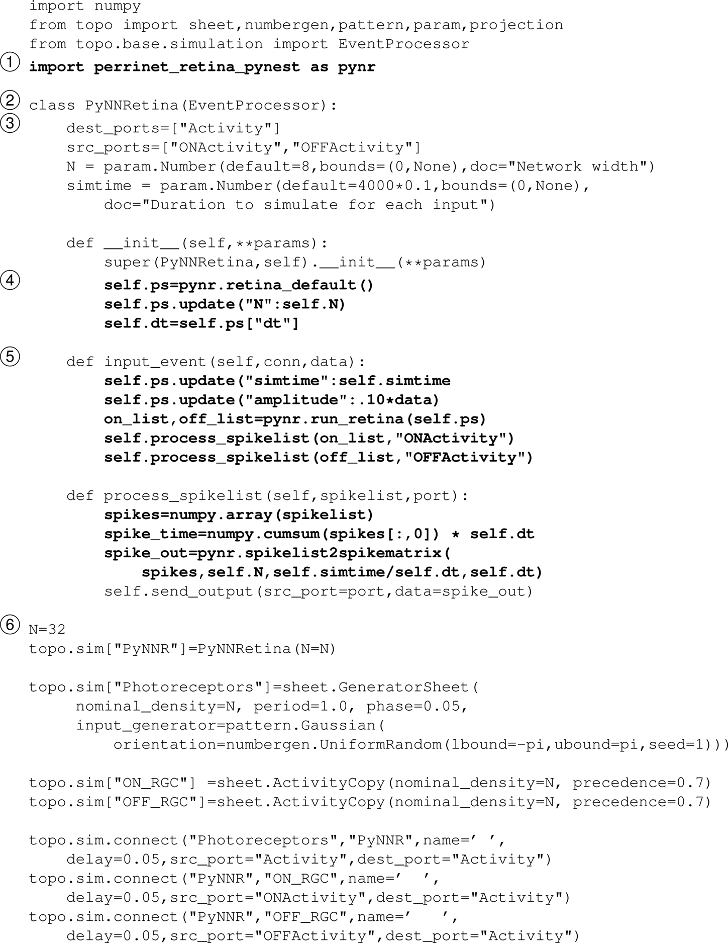
Figure 3. Sample Topographica interface code. This Python code shows a complete, runnable Topographica 0.9.6 simulation interfacing with an external PyNN/PyNEST spiking simulation of ON and OFF retinal ganglion cells. The text in bold starts the PyNN simulation and retrieves the results, and would need to be changed for interfacing to a new external simulation. The other text sets up an appropriate Topographica simulation framework, and only needs changing to e.g. match the number and type of sheets that you want to expose from the underlying external simulation.
 First, the external simulation is imported, making anything available to Python from that simulation also available to Topographica. For this import to succeed, PyNN, NEST, and PyNEST need to be installed, and each need to have been given Topographica’s copy of Python during installation so that they will be available to Topographica.
 Next, we define a new type of Topographica EventProcessor
 PyNNRetina to handle communication between Topographica and the external simulator. This class simply accepts an incoming event from Topographica that contains a matrix of photoreceptor activity, passes the matrix to the external spiking simulator, collects the firing-rate-averaged results, and sends them out to any Topographica sheets that may be connected. More specifically, the class first declares that it can accept an incoming event on a port labeled
 Activity, and that it will generate two separate types of output data to be made available on the ONActivity and OFFActivity dest_ports. It also declares that it has two user-controlled parameters, N (size of array of neurons) and simtime (duration to run the simulation for each input). (Additional parameters from the underlying simulator can be declared similarly, or all of the underlying parameters could be exposed as a batch using suitable gluing code.) The constructor (
--init--) does any initialization that should be done once per run, here consisting only of defining some parameters, but potentially including launching an external simulator, making a connection to a remote simulator already running, etc. The
The input_event method is called by Topographica whenever an Event delivers data to this object’s src_port (Activity). In this case, the method adds the incoming activity matrix into its parameters data structure (ps), and then calls the external function run_retina to run the underlying simulation. When the external simulator completes, two lists of spikes are returned, one for ON and one for OFF, and these are processed using the helper function process_spikelist. For each list, process_spikelist computes the firing rate of each neuron and sends the resulting floating-point arrays out the appropriate port. The remainder of the code instantiates a model network to display the results from this class, defining one
 PyNNR object, a Photoreceptors Sheet to generate input patterns, two RGC Sheets to display the resulting activity patterns, and connections between them.Running this model (or other Python-based simulations) within Topographica adds only a tiny amount of computational cost. For this example running on a 3GHz Intel Core 2 Duo machine, simulating in batch mode with N=8 and simtime=4 s takes 16.07 s in Topographica, versus 15.88 s using the native PyNN version (averages of 5 trials; variance negligible). This 0.2-s time difference consists mainly of libraries that Topographica imports when it starts up, and the ongoing cost is normally negligible for a non-trivial external Python model.
With this interface in place, the external simulation can be used with nearly all of Topographica’s features. For instance, Figure 4
shows one example input pattern and the resulting pattern of ON and OFF RGC activity. For this example, the main benefit to having the Topographica wrapper is to be able to present any of the types of input patterns in Topographica’s large library of input patterns, using either the GUI so that the results can be seen interactively, or systematically using Python code. For other simulations, e.g. those including cortical areas such as V1, Topographica can compute tuning curves, receptive fields, many types of preference maps, and other analyses and plots for any of the neurons and Sheets available to Topographica, with no coding required. As long as the computation only requires average firing rates, no special-purpose code or additional interface will be needed beyond what is shown in this example. Thus Topographica can be used to provide a consistent set of analyses and plots for a wide variety of underlying simulations.
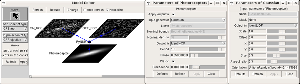
Figure 4. Example architecture. This figure shows the simulation from Figure 3
running in Topographica. On the input sheet is a 2D Gaussian pattern generated by Topographica and presented to the underlying spiking network, with the resulting spike count responses shown on the ON and OFF RGC sheets. The type of input pattern and its parameters can be manipulated as shown.
Interfacing to other Python Code (e.g., PyNEST, Neuron)
The general approach outlined in the section “Interfacing to Perrinet Retinal Model in PyNN” can be used for any other model running in an external simulator that has a Python interface or is written directly in Python. In each case, a new Topographica EventProcessor class can be created to accept incoming events, process them somehow, and generate appropriate output. For instance, similar steps would have been used if the retina model had been written in PyNEST directly rather than PyNN, or in NEURON’s own Python interface. As long as the external simulator can be told to use Topographica’s copy of Python, then Topographica can import the required functions, execute them as part of such a class, and thus control its input and output. As a result, the main issues with interfacing to other Python-based simulators are not so much technical as conceptual; these conceptual issues will be reviewed in the “Discussion” section.
Interfacing to Matlab
Topographica can also connect easily to external simulations running in Matlab, using the Python ↔ Matlab interface package
mlabwrap
3
that is supplied with Topographica.For instance, the following complete, runnable Topographica script defines a Python/numpy array a and then calls a Matlab function “nestedsum” on it:
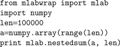
Here nestedsum.m is an arbitrary example of a Matlab function placed somewhere in Matlab’s path, containing:
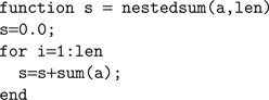
(This code prints
5.0000e+14 when run from Matlab, and 4.99995000e+14 when run from Topographica/Python.) Any built-in or user-supplied Matlab function can be called similarly (including plotting code like mlab.plot(a)), with nearly seamless interchange of scalar and array data between the two systems. This capability makes it simple to develop interfaces like that in the section “Interfacing to Perrinet Retinal Model in PyNN”, or just to use small bits of Matlab code or visualizations when appropriate.The mlabwrap package performs some data conversion behind the scenes, but the overhead is still usually negligible. The example above run on the same machine as for PyNN takes 12.27 s in Topographica, versus 11.57 s for a pure Matlab version. Again, this 0.7 s difference includes the entire startup time, and increases little with simulation size (e.g. 0.8 s out of 44 for
len=200000).The main technical limitation of the mlabwrap Matlab interface is that at present it only supports 1D and 2D arrays, because the mlabwrap author has not yet added n-dimensional array support. More importantly, interfacing to external Matlab models can be difficult because of the monolithic (as opposed to object-oriented) programming style typically used for Matlab programming. For instance, the Olshausen and Field (1996)
model available from
4
is a good match to Topographica conceptually, but running it within Topographica in a useful way requires splitting up the Matlab code into three components to handle the input pattern generation, response to the input, and the weights update separately. These functions were originally controlled by a single Matlab script. Thus in practice how difficult it would be to interface to Matlab code depends on the programming style and complexity, with simple functions being simple to access but complicated models potentially requiring prior reorganization on the Matlab side.
Interfacing to C/C++
Python offers a wide variety of methods for interfacing to C or C++ code, any of which could be used with Topographica. The specific interface currently used for the performance-critical portions of Topographica is Weave
5
, which allows snippets of C or C++ code to be called easily from within Python code. A sample complete, runnable Topographica/Python script with C code is:
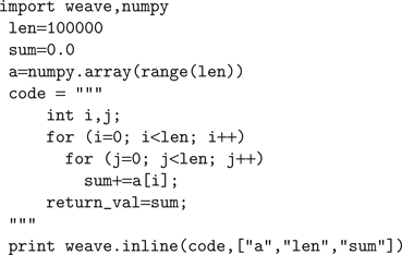
Here the C code in the string named
code is computing the same function as the Matlab code above; it will print 4.99995e+14 when run. The first time it is run the C compiler will be called automatically to compile that code fragment, and then the saved object file will be reused in subsequent calls and on subsequent runs, unless the C code string is changed. This approach makes it simple to include bits of existing C code to optimize specific functions, or to make calls to C libraries.The C interface adds very little overhead, in part because it uses numpy arrays in place. The example above takes 10.34 s in Topographica, versus 10.07 for a pure C equivalent. This 0.3-s difference is primarily due to the Topographica startup time, because it does not increase with simulation size or length. Also note that the full C version must be recompiled for any change, even trivial ones, while the Topographica/Python version only recompiles when the code string changes (which is typically rare if C is used only for performance-critical sections; recompilation adds about 1 s to the runtime in this example).
Using weave in this way makes it simple to add small bits of C code, but other approaches such as
ctypes (included in Python 2.5) can be more suitable for interfacing to large external C packages. Again, how difficult the interface will be depends on whether the external code is arranged into entities that can be called directly from Topographica; as discussed below, reorganizing the code in this way is usually straightforward but can take some effort.As the examples above show, very little coding is required to wrap even complex simulations into the basic Sheet and EventProcessor components used in Topographica. A large class of models across different modelling and analysis levels (e.g., firing-rate, integrate-and-fire, and compartmental neuron models) can fit into this structure, allowing all of them to be analyzed and compared consistently, interconnected where appropriate, and explored visually even if the underlying simulator has no graphical interface (as for NEST). Although the general problem of simulator interoperatibility is difficult to address, in this specific case it is relatively easy to get practical benefits from combining simulators.
Although the approach outlined above is general purpose, it does require coding a new Topographica component to match each specific model implemented externally. A useful but more complex alternative would be to provide a detailed mapping between object types in an external simulator. For instance, one could provide a Topographica Sheet object that instantiates a corresponding NEST layer object, and similarly for a Topographica Projection object and a NEST connection object. In this way NEST or other simulators could be used to provide specific functionality missing from Topographica, rather than to implement complete models. However, developing such interfaces is much more involved than the simple wrapping described here.
Even though the Topographica Sheet interface is general enough to fit a wide range of current models, there are some models that do not fit within its assumptions. In particular, a Sheet usually needs to have an underlying grid shape to the population of neurons, though individual neurons can be absent or at jittered spatial locations, as long as no more than one neuron is present in any grid cell. (Strictly speaking, it need only be possible to visualize the model in this way; the actual organization is arbitrary.) Also, only Cartesian grids are currently supported, though hexagonal grids could be added in the future. Arbitrary 3D locations will be difficult to support, except by imposing a 3D grid. Note that nonlinear spacings are supported, using arbitrary coordinate mapping between Sheets, e.g. for foveated retinotopic mappings, as long as there is still an underlying grid of neurons.
Apart from operating loosely on a grid, Topographica assumes that models will have regions that are separable from each other, communicating only over well defined channels, and usually incrementally processing some sort of external stimuli that change over time. Although these assumptions are extremely general, and can apply to any physical system, many models do not satisfy them fully. For instance, models that represent inputs not as individual patterns but as correlation functions (e.g. Miller, 1994
) are difficult to connect to Topographica, because most of the functionality of Topographica requires testing the response to specific external stimuli (e.g. for measuring maps, tuning curves, and receptive fields). Other types of models that operate in a “batch” mode rather than one pattern at a time (e.g. Olshausen and Field, 1996
) can usually be adapted to work in incremental mode as required by Topographica, but they may then run much more slowly.
Given the ease with which many models can be wrapped, an intermediate-term goal will be to provide example code for wrapping as many current V1 models as possible into Topographica, to establish for the first time a platform for evaluating their behavior and functionality consistently. At present, each model is implemented independently, with different analysis routines and types of visualization, and thus it is extremely difficult to determine if apparent differences in behavior are significant. As long as runnable code is available for each model, wrapping it into Topographica should be straightforward and should provide immediate benefits.
In addition to interfacing with external model components, any of the mechanisms outlined above can be used to call externally defined general-purpose analysis or visualization functions. For instance, the NeuroTools package
6
defines an object-based Python representation of spike trains, such as those used in the spiking retina model above. A native spiking Topographica model can then use these functions rather than reimplementing them within Topographica.
This paper focuses on making external simulations available within Topographica, to allow simulations at the topographic map level or at lower levels to be brought into a common analysis and testing framework. It is also straightforward to interface in the opposite direction, running a Topographica simulation from within an external system or simulators. The Topographica User Guide
7
provides detailed examples of running models from the Python command line or Python scripts, and the same interface can be used from within any simulator that has Python bindings. Moreover, Topographica has a highly modular design with few dependencies between components, and there are many Topographica objects that are useful on their own and can be used just as any other Python object from within an external program.
At present, Topographica is primarily useful for doing analyses based on firing rates, because of its extensive firing-rate based libraries. Spiking simulations are also possible in Topographica, but they are currently quite limited, and will require additional work to establish general-purpose abstractions that can be used to integrate data across models and simulators. In the long run, we intend Topographica to be useful as a high-level platform for analyzing spiking output as well as firing-rate output, and would welcome collaborations with people interested in that topic or in other aspects of Topographica or interoperability development.
In summary, working at the topographic map level makes it practical to provide interconnections between models and simulators working at the same or different levels of detail. As long as the neurons are grouped into two-dimensional sheets of related units, they will be able to interface easily with Topographica’s tools and components. The result provides a shared platform for evaluating models from different sources, allowing consistent analysis and testing even for very different implementations. We believe this shared, extensible tool will be highly useful for the community of researchers working to understand the large-scale structure and function of the nervous system.
The authors declare that the research was conducted in the absence of any commercial or financial relationships that could be construed as a potential conflict of interest.
Supported in part by the National Institutes of Mental Health under Human Brain Project grant 1R01-MH66991, by the National Science Foundation under grant IIS-9811478, and by the EPSRC/MRC Doctoral Training Centre in Neuroinformatics at the University of Edinburgh. Thanks to Laurent Perrinet (INCM/CNRS) for contributing his retina model as an example, for assisting with the process of interfacing it to Topographica, and for making comments on an earlier draft of this manuscript. Thanks also to all of the Topographica developers, particularly Christopher Ball, without whom this work would not have been possible.
Bednar, J. A. (2008). Understanding neural maps with topographica. In Interactive Educational Media for the Neural and Cognitive Sciences. Brains, Minds and Media, Vol. 3, bmm # 1402, S. Lorenz and M. Egelhaaf (eds). http://www.brains-minds-media.org/archive/1402
.