Inter-subject correlation of brain hemodynamic responses during watching a movie: localization in space and frequency
1
Department of Signal Processing, Tampere University of Technology, Tampere, Finland
2
Department of Biomedical Engineering and Computational Science, Aalto University School of Science and Engineering, Espoo, Finland
Cinema is a promising naturalistic stimulus that enables, for instance, elicitation of robust emotions during functional magnetic resonance imaging (fMRI). Inter-subject correlation (ISC) has been used as a model-free analysis method to map the highly complex hemodynamic responses that are evoked during watching a movie. Here, we extended the ISC analysis to frequency domain using wavelet analysis combined with non-parametric permutation methods for making voxel-wise statistical inferences about frequency-band specific ISC. We applied these novel analysis methods to a dataset collected in our previous study where 12 subjects watched an emotionally engaging movie “Crash” during fMRI scanning. Our results suggest that several regions within the frontal and temporal lobes show ISC predominantly at low frequency bands, whereas visual cortical areas exhibit ISC also at higher frequencies. It is possible that these findings relate to recent observations of a cortical hierarchy of temporal receptive windows, or that the types of events processed in temporal and prefrontal cortical areas (e.g., social interactions) occur over longer time periods than the stimulus features processed in the visual areas. Software tools to perform frequency-specific ISC analysis, together with a visualization application, are available as open source Matlab code.
Inter-subject correlation (ISC) analysis (Hasson et al., 2004
) is a model-free approach to examine the highly complex functional magnetic resonance imaging (fMRI) data acquired in natural, context-dependent, audiovisual stimulus environments, such as during watching movies. In the ISC analysis, hemodynamic activity of a reference subject is used to predict the hemodynamic activity of another subject in corresponding voxels by calculating the correlation coefficient between the hemodynamic activity time series. One of the major benefits of the ISC analysis is that it can be used to locate activated brain areas without a priori knowledge of the temporal composition of processes contributing to the measured signals as inferences are solely based on the similarities in hemodynamic responses across subjects. In recent studies, ISC analysis has been applied, for example, to disclose hemodynamic activity elicited by watching movies (Hasson et al., 2004
; Golland et al., 2007
; Jääskeläinen et al., 2008
; for a review, see Hasson et al., 2010
), narrative speech comprehension (Wilson et al., 2008
), auditory abnormalities (Hejnar et al., 2007
), and episodic memory encoding (Hasson et al., 2008a
). For example, a study where five participants viewed a 30-min clip of the western movie “The Good, The Bad, and The Ugly” (directed by Sergio Leone, Metro-Goldwyn Mayer Films, 1966) significant ISC was revealed in sensory specific cortices, the fusiform gyrus, and the limbic system (Hasson et al., 2004
). However, prefrontal cortical areas appeared to lack ISC in this early study (Hasson et al., 2004
). In our recent study, we first showed volunteers a major part of the movie “Crash” (directed by Paul Haggis, Lions Gate films, 2005) outside of the fMRI scanner to provide them with the full context of the plot and to get them emotionally involved prior to showing them the last 36 min during fMRI scanning (Jääskeläinen et al., 2008
). In this setting, we observed also significant frontal-cortical ISCs between pairs of subjects. Prefrontal cortical ISC was also recently observed when subjects watched a television episode of Alfred Hitchcock Presents (Bang! You’re Dead, 1961, directed by Alfred Hitchcock) (Hasson et al., 2008b
).
Stimuli and events unfold in our natural environments over multiple time-scales. Elementary features of visual stimuli, for example, change over very short time-scales compared to spoken sentences, perceiving social interactions and development of social relationships that evolve over progressively longer time periods. Thus, the brain needs to process information across various time-scales. A recent fMRI study, where short silent movie clips and their corresponding time-scrambled and reverse-played versions were used as stimuli, suggested that temporal receptive windows (TRWs) in the human cortex are not homogeneous across brain regions. Rather, visual sensory areas were observed to have quite short time windows over which information is integrated, and hierarchically higher-order areas, such as parieto-temporal cortical areas and frontal eye field, were observed to have longer TRWs (Hasson et al., 2008c
). Specifically, the TRW lengths were inferred from the effect that disruptions in temporal structure, caused by the re-sequencing/time scrambling of the movie clips over different time-scales, had on response reliability in different cortical areas. While the early visual areas exhibited high response reliability regardless of disruptions in temporal structure, response reliability in the higher-order cortical areas depended on intactness of temporal order of events in the movie clips over longer time-scales (Hasson et al., 2008c
). Findings of progressively longer sensory adaptation time-scales with increasing level of cortical hierarchy (Lü et al., 1992
; Uusitalo et al., 1997
; Raij, 2008
) support this view.
Here, we investigated processing of movie events that occur over multiple time-scales. Our approach differed from that of Hasson et al. (2008c)
in that instead of using silent time- scrambled movie clips, we inspected ISCs over distinct frequency bands in a fMRI dataset from our previous study (Jääskeläinen et al., 2008
), which was collected while 12 healthy volunteers watched the last 36 min of an Academy Award winning movie “Crash” that was presented with sound (Lions Gate Films, 2005, directed by Paul Haggis). We expected these data to be especially suitable for the study of temporal organization across the brain since significant ISCs occurred in both sensory areas and higher-order frontal cortical areas. We hypothesized that the low-frequency component of the ISC is dominant in higher-order cortical areas involving integration of information over long time-scales (i.e., that the type of events that higher-order cortical areas process occur over longer time windows in the movie), whereas sensory areas such as early visual cortex would be dominated by higher-frequency ISCs due to the relatively transient nature of the elementary visual features that the early visual areas are sensitive to. We decomposed fMRI data into several frequency sub-bands and then performed a group-level ISC analysis separately within each frequency band. A filter bank was implemented using stationary wavelet transformation (SWT), which is straightforward to apply to any fMRI dataset. We further present two nonparametric permutation-based procedures to make inferences about ISCs: one to assess (1) whether there is significant ISC within a specific frequency band and (2) whether ISC differs between two frequency bands. The frequency-specific ISC was implemented with MATLAB and the source code, together with the interactive visualization tool, is openly available to the neuroscience community (see Supplementary Material).
Frequency-based ISC is a model-free technique that is especially suited for the analysis of fMRI data obtained during complex naturalistic stimulation. A general concept of the frequency-specific ISC is presented in Figure 1
. First, fMRI time-series of two or more subjects are compared on a voxel-by-voxel basis with a chosen similarity criterion over the whole brain (Figure 1
, left). Frequency-dependent information is included in the analysis by first filtering each fMRI time-series using an appropriate filter bank, and then repeating across-subject similarity calculations separately within every frequency sub-band (Figure 1
, right). In order to investigate similarities at the group level, pair-wise correlations between all subject pairs are combined into a single statistic describing average similarity over the group of subjects. Two different non-parametric permutation tests are then used to make statistical inferences about the voxel-wise statistic: one to assess significance of the ISC within a single frequency sub-band, and one to assess whether ISCs in two frequency bands differ. A separate test of the ISC difference between two frequency bands is required because presence of significant ISC in one frequency band and absence in another frequency band does not necessarily mean that the effect between these two bands is significantly different. The conclusion that there is a difference between two conditions when the activation is present in one comparison and absent in another comparison is a common misinterpretation in neuroimaging literature known as “imager’s fallacy” (Henson, 2005
; Poldrack et al., 2008
).
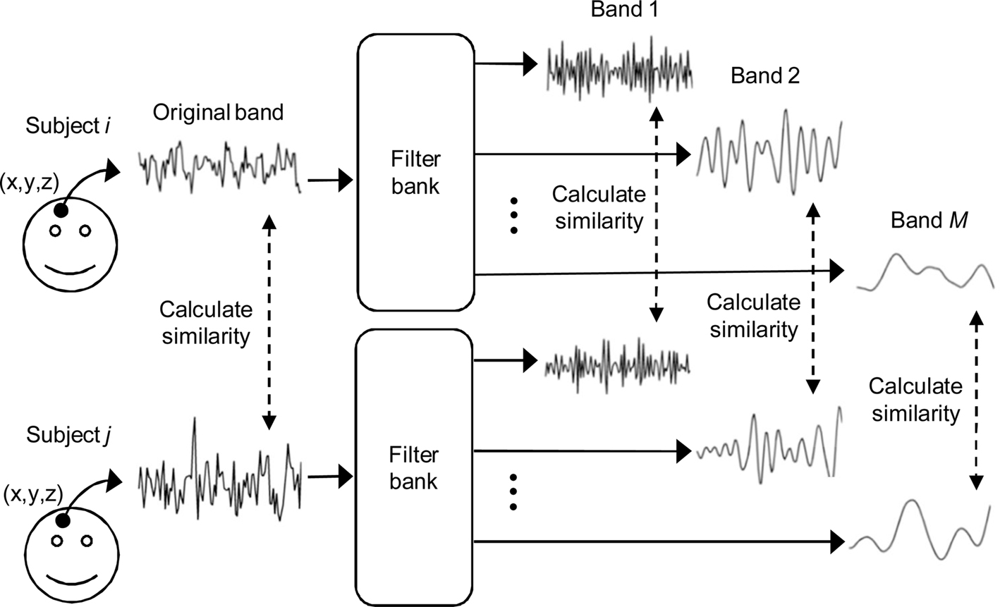
Figure 1. General concept of frequency-specific ISC analysis. Voxel-by-voxel ISC is calculated across subjects over the original fMRI time-series as well as over several frequency sub-bands. The method is extended to a multi-subject analysis by combining the results of each subject pair into a single statistic representing an average across-subject similarity.
We implemented frequency-specific ISC with MATLAB, and designed an interactive software tool for browsing and visualization of the analysis results. Source code for performing frequency-specific ISC together with the interactive visualization tool is freely available (see Supplementary Material).
Natural Viewing Experiment
We reanalyzed data from our recent natural viewing experiment (Jääskeläinen et al., 2008
). fMRI was measured from 15 healthy right-handed volunteers (age range 19–44, seven females, data from three subjects was discarded previously due to bad quality) when they watched the movie “Crash” (directed by Paul Haggis, Lions Gate Films, 2005). Ethical approval was granted by the Coordinating Ethical Committee of Hospital District of Helsinki and Uusimaa, Finland. The study was run in accordance with the guidelines of the Helsinki declaration, and a written voluntary consent was obtained prior to participation in the study from each subject. A General Electric Signa 3 Tesla MRI scanner with Excite upgrade located in the Advanced Magnetic Imaging Center at the Helsinki University of Technology was used in recordings. The movie was selected because of its high quality (reflected in three Academy Awards in 2006: best picture, film edit, writing/screenplay), and because it had been identified in the initial screening process as one eliciting strong emotions in viewers. Only those subjects who had not seen the movie previously and who were fluent in English were accepted to the study since the language of the movie was English. In the beginning of the experiment, each subject watched the first 72 min of the movie on a LCD screen in a dimly lit room with a five-speaker surround-sound setting. The movie was then discontinued and the subject was prepared for the fMRI scans, which took about 30 min. In the beginning of the scanning process, initial localizer scan and 45 axial T1-weighted anatomical MRI slices (slice thickness 5 mm, in-plane 2 mm × 2 mm) were acquired. During functional imaging, the movie was projected onto a translucent screen, which the subjects viewed through an angled mirror, and the audio track of the movie was played to the subjects via a pneumatic audio system with earplugs. The last 36 min of the movie were shown for a subject in two parts lasting 14 and 22 min, respectively, with a pause of about 30 s in between. The break was due to limitations in the number of slices that could be acquired during a single run in the MRI scanner that was used (Jääskeläinen et al., 2008
). Altogether 630 whole-brain T2* weighted gradient echo EPI volumes (TR = 3400 ms, TE = 32 ms, flip angle 90°, 52 axial slices, 3 mm slice thickness without gaps, 3 mm × 3 mm in-plane resolution) were acquired during the two movie clips. T2-weighted fluid attenuated inversion recovery and high resolution 3D T1-weighted structural images were obtained immediately after the presentation. The subjects were instructed not to move during the scanning session in order to avoid motion artifacts.
Image Preprocessing
We preprocessed the original fMRI experiment data of 12 subjects using the FSL software library (FMRIB, Oxford University; Smith et al., 2004
). Since we wanted to avoid any discontinuities in the data, we processed and analyzed the two scanning sessions separately. First, motion correction was performed by using MCFLIRT (Jenkinson et al., 2002
). Time-series were then detrended using a nonlinear Gaussian weighted least-squares fitting with a cutoff of 100 s, and spatial smoothing was applied with a Gaussian kernel with FWHM of 5 mm. Note that the detrending removes only a part of the low frequency signal components (we observed approximately 10% signal energy loss below the cutoff frequency) and it is reasonable to study the frequency bands below the cutoff value after the detrending. After preprocessing, images were spatially normalized to the ICBM-152 template using the FLIRT registration tool (Jenkinsson and Smith, 2001
). Skull-stripped functional images were first aligned (six-parameter rigid transformation) to the skull-stripped high-resolution T1-weighted image of the same subject, and then the T1-weighted image to the standard (brain only) ICBM-152 template with a 12-parameter affine transformation. The skull-stripping of functional images was performed with BET (Smith, 2002
). T1-weighted images were skull-stripped using a customized procedure involving genetic algorithm based voxel classification (Tohka et al., 2007
) and brain extraction from the voxel classified images using Brain Surface Extractor (Shattuck et al., 2001
).
Filter Bank Construction with Stationary Wavelet Transform
Multiresolution analysis using discrete wavelet transform (DWT) is a widely used technique to analyze time-scale characteristics of discrete-time signals and to construct octave-filter banks (Mallat, 1999
). In fMRI signal analysis, wavelets have been advocated for several reasons. For example, wavelet analysis is a prominent approach when analyzing fractal signals or signals with 1/f -like frequency characteristics, both properties that have been associated with cortical resting-state fMRI time-series (Bullmore et al., 2004
; Maxim et al., 2005
). The standard implementation of DWT uses a sub-band coding scheme consisting of successive stages of filtering and down-sampling (for a detailed description, see Vetterli and Kovačević, 2007
). However, the down-sampling makes DWT time variant (i.e., DWT is not time-invariant). This means that even a minor shift in the input signal can cause large changes in the transformed signal (Bradley, 2003
). The lack of time-invariance is problematic for the ISC analysis because even a small difference in hemodynamic responses between two subjects can lead to inconsistencies in the estimation of correlation between the subjects’ time courses.
We constructed a wavelet filter bank using a closely related technique called SWT, also known as undecimated wavelet transform, redundant wavelet transform, or maximum-overlap DWT (MODWT) in the literature, to overcome the problems associated with DWT. Previously, SWT has been used to investigate resting-state fMRI data by Achard et al. (2006)
. SWT is a time-invariant transformation and therefore a good choice for frequency-specific ISC analysis. In SWT, a signal of interest is not downsampled but instead the analysis filter coefficients are upsampled after successive filtering steps (Nason and Silverman, 1995
). Because the number of samples in successive decomposition levels remains constant, SWT leads to an overdetermined representation of the original time-series – hence the name redundant wavelet transform. Next, we briefly describe the algorithm to perform SWT (known as algorithme à trous; Vetterli and Kovačević, 2007
) to highlight its good properties for the frequency-specific ISC analysis. Let H denote a unit length low-pass filter whose coefficients {h[n]} satisfy the following internal orthogonality relation (Nason and Silverman, 1995
):

and let G denote a high-pass filter having coefficients {g[n]} satisfying:
Also the filter G satisfies (1) and together the filters H and G are called a quadrature mirror filter (QMF) pair. To derive SWT, two operations are required. First, we define a filtering operation applied to a sequence x as a convolution sum:
where boundary conditions are treated using periodic signal extension. Second, we define the operator Z that alternates zeros in a discrete sequence x in such a way that for all integers j, (Zx)[2j] = x[j] and (Zx)[2j + 1] = 0. Now, assume that a low-pass filter H(r) has the coefficients Zrh, i.e., hr[k] = h[j] if k = 2rj, and hr[k] = 0 if k ≠ 2rj. Clearly, the filter H(r) can be obtained by inserting zeros between every adjacent pair of elements of the filter H(r−1). Similarly to H(r), we define a high-pass filter G(r) having coefficients Zrg. Then, denoting the original signal by c0[n], SWT is computed by applying recursively the following operations for j = 1,2,…,J:

Here, cj[n] and dj[n] stand for approximation and detail coefficients at scale j, respectively, and J is the number of decomposition scales.
We wrote customized MATLAB code to implement 4-scale (J = 4) SWT decomposition using Daubechies 2 QMF pair to filter the fMRI time-series of each subject. With the 4-scale filter bank, five frequency sub-bands were obtained, consisting of four sets of detail (d1[n], d2[n],d3[n], d4[n]) and one set of approximation coefficients (c4[n]). The decomposition scheme is illustrated in Figure 2
. For notational convenience, we denote decompositions by sk[n] = dk[n], for k = 1,2,3,4, and sk[n] = ck[n] for k = 0,5.
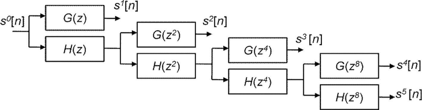
Figure 2. Decomposition of discrete signal s0[n] using 4-scale SWT.
Table 1
displays approximate frequency characteristics and the corresponding time-scales of the fMRI time-series after the wavelet decomposition. The successive splitting of the low pass-filtered coefficients into new low- and high-pass coefficients leads to a logarithmic scale of the frequency sub-bands.
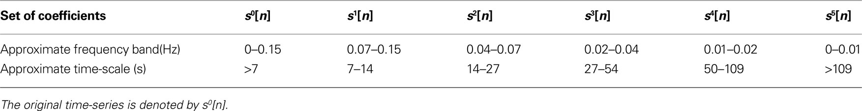
Table 1. The frequency characteristics of the constructed wavelet filter bank.
Frequency-Specific Intersubject Correlation Analysis
We used Pearson’s correlation coefficient to derive our multi- subject similarity measure. First, we calculated voxel-wise temporal correlation between every pair of subjects within each frequency band as:
where N is a total number of samples in time-series, rij is the sample correlation coefficient between the time-series si and sj obtained from the ith and jth subject, respectively, and  and
and  denote the mean values of si and sj. Note that superscripts denoting frequency sub-bands are omitted from Eq. 2 for simplicity. Then, we combined rij values from all subject pairs into a single ISC statistic by averaging:
and denote the mean values of si and sj. Note that superscripts denoting frequency sub-bands are omitted from Eq. 2 for simplicity. Then, we combined rij values from all subject pairs into a single ISC statistic by averaging:
where m is the number of subjects. Thus, as m was 12 in our study, we averaged correlation coefficients of (122 − 12)/2 = 66 subject pairs. The statistical inference is complicated by the dependency of the 66 correlation coefficients. Wilson et al. (2008)
suggested a t-test based approach for testing if the sum of Z-transformed intersubject correlation coefficients is different from 0. The parametric form of the null distribution was verified using a goodness-of-fit evaluation based on permutation testing. Because we had adequate computational resources available and the statistic has an intuitive meaning when examining intersubject similarities, we performed a fully nonparametric voxel-wise permutation test for  statistic similar to the goodness of fit evaluation of Wilson et al. (2008)
. The test was performed against the null hypothesis that
statistic similar to the goodness of fit evaluation of Wilson et al. (2008)
. The test was performed against the null hypothesis that  statistic is the same as for unstructured data, which would be expected if there was no ISC present. To generate the permutation distribution, we circularly shifted each subject’s time-series by random amount so that they were no longer aligned in time across the subjects, and then calculated
  statistic. This way we could account for temporal autocorrelations present in the fMRI data. Because calculation of all the possible time shift combinations would be computationally prohibitive, we approximated the full permutation distribution with A = 100,000,000 realizations. Sampling was randomized over every brain voxel, frequency sub-band and shifting point without any restrictions. We corrected the resulting p-values using false discovery rate (FDR) based multiple comparisons correction with independence or positive dependence assumption (Benjamini and Hochberg, 1995
; Nichols and Hayasaka, 2003
). FDR corrected thresholds were calculated separately for each frequency sub-band. We calculated two permutation distributions to threshold frequency-dependent ISC maps of the both scanning sessions (separate distributions are needed because of different numbers of data points available to compute the correlation coefficients).
statistic. This way we could account for temporal autocorrelations present in the fMRI data. Because calculation of all the possible time shift combinations would be computationally prohibitive, we approximated the full permutation distribution with A = 100,000,000 realizations. Sampling was randomized over every brain voxel, frequency sub-band and shifting point without any restrictions. We corrected the resulting p-values using false discovery rate (FDR) based multiple comparisons correction with independence or positive dependence assumption (Benjamini and Hochberg, 1995
; Nichols and Hayasaka, 2003
). FDR corrected thresholds were calculated separately for each frequency sub-band. We calculated two permutation distributions to threshold frequency-dependent ISC maps of the both scanning sessions (separate distributions are needed because of different numbers of data points available to compute the correlation coefficients).
statistic similar to the goodness of fit evaluation of Wilson et al. (2008)
. The test was performed against the null hypothesis that statistic is the same as for unstructured data, which would be expected if there was no ISC present. To generate the permutation distribution, we circularly shifted each subject’s time-series by random amount so that they were no longer aligned in time across the subjects, and then calculated statistic. This way we could account for temporal autocorrelations present in the fMRI data. Because calculation of all the possible time shift combinations would be computationally prohibitive, we approximated the full permutation distribution with A = 100,000,000 realizations. Sampling was randomized over every brain voxel, frequency sub-band and shifting point without any restrictions. We corrected the resulting p-values using false discovery rate (FDR) based multiple comparisons correction with independence or positive dependence assumption (Benjamini and Hochberg, 1995
; Nichols and Hayasaka, 2003
). FDR corrected thresholds were calculated separately for each frequency sub-band. We calculated two permutation distributions to threshold frequency-dependent ISC maps of the both scanning sessions (separate distributions are needed because of different numbers of data points available to compute the correlation coefficients).In addition to  , we calculated indexed ISC maps to visualize the frequency bands showing the highest ISC (according to Eq. 3). For these maps, the frequency band index was calculated for each voxel as follows:
, we calculated indexed ISC maps to visualize the frequency bands showing the highest ISC (according to Eq. 3). For these maps, the frequency band index was calculated for each voxel as follows:
where a  {1,2,3,4,5} indexes a frequency band. The maps were thresholded according to the lowest FDR corrected threshold among the frequency bands, since FDR correction leads to a separate threshold for each frequency band. Investigation of the frequency-specific permutation distributions showed that standard deviations in lower frequency bands were greater compared to those of higher frequency bands. This was expected, because time resolution decreases when moving from higher frequencies towards the lower ones. Difference in standard deviations across the frequency bands is not problematic when investigating individual ISC maps because FDR correction is performed separately for each frequency band. When investigating results simultaneously across several frequency bands, it must be noticed that it is more likely to see spurious ISC values in lower frequency bands compared to higher ones. However, the investigation of the mean values of the frequency-specific permutation distributions showed that the ISC values were not inflated due to filtering (the range of the mean distribution values in different frequency bands was from −4.06 × 10⁻⁵ to −1.96 × 10⁻⁶ for the first scanning session, and from −2.67 × 10⁻⁵ to 2.34 × 10⁻⁵ for the second scanning session), indicating that it is reasonable to investigate multi-frequency mappings as proposed in Eq. 4.
{1,2,3,4,5} indexes a frequency band. The maps were thresholded according to the lowest FDR corrected threshold among the frequency bands, since FDR correction leads to a separate threshold for each frequency band. Investigation of the frequency-specific permutation distributions showed that standard deviations in lower frequency bands were greater compared to those of higher frequency bands. This was expected, because time resolution decreases when moving from higher frequencies towards the lower ones. Difference in standard deviations across the frequency bands is not problematic when investigating individual ISC maps because FDR correction is performed separately for each frequency band. When investigating results simultaneously across several frequency bands, it must be noticed that it is more likely to see spurious ISC values in lower frequency bands compared to higher ones. However, the investigation of the mean values of the frequency-specific permutation distributions showed that the ISC values were not inflated due to filtering (the range of the mean distribution values in different frequency bands was from −4.06 × 10⁻⁵ to −1.96 × 10⁻⁶ for the first scanning session, and from −2.67 × 10⁻⁵ to 2.34 × 10⁻⁵ for the second scanning session), indicating that it is reasonable to investigate multi-frequency mappings as proposed in Eq. 4.We also investigated variability of the frequency-specific ISC results across the two scanning sessions. We quantified across- session reproducibility within each frequency band by calculating a mean absolute error between the two sessions across every brain voxel as follows:

where  and
and  stand for
  statistic (Eq. 3) across the first and the second scanning session, respectively, and B denotes the set of all brain voxels. There are many sources of variability contributing to the absolute error, including different stimuli during two scanning sessions. Therefore, the interpretation of the variability measure is not straight-forward. However, we wished to provide a quantitative measure of the scanning session differences in addition to qualitative inspection of the statistical parameter maps.
and stand for statistic (Eq. 3) across the first and the second scanning session, respectively, and B denotes the set of all brain voxels. There are many sources of variability contributing to the absolute error, including different stimuli during two scanning sessions. Therefore, the interpretation of the variability measure is not straight-forward. However, we wished to provide a quantitative measure of the scanning session differences in addition to qualitative inspection of the statistical parameter maps.Frequency-Band Comparison
We designed a permutation test also to assess whether ISC in one frequency band differs significantly from ISC in another frequency band. First, we used the modified Pearson–Filon statistic based on Fisher’s z transformation (ZPF) (Raghunathan et al., 1996
) to compare ISC across frequency bands between two subjects, which is a recommended test statistic for two, non-overlapping dependent correlations (Krishnamoorthy and Xia, 2007
). A selection of the statistic was based on the assumption that subject-pairwise correlation coefficients may be correlated in distinct frequency sub-bands. To obtain ZPF statistic, all pairwise correlation coefficients (obtained by Eq. 2) were first transformed into a normally distributed form through Fisher’s z transformation:
where superscript a refers to the frequency band. The difference between the two z transformed correlation coefficients was then transformed into a ZPF statistic through the following transformation (Raghunathan et al., 1996
):
With certain assumptions, the ZPF statistic is distributed according to the standard normal distribution N(0,1) under the null hypothesis of no difference between the correlation coefficients. Here, notation  stands for correlation between the time-courses of ith subject from frequency band a and jth subject from frequency band b, and large-scale covariance is given by Raghunathan et al. (1996)
:
stands for correlation between the time-courses of ith subject from frequency band a and jth subject from frequency band b, and large-scale covariance is given by Raghunathan et al. (1996)
:
stands for correlation between the time-courses of ith subject from frequency band a and jth subject from frequency band b, and large-scale covariance is given by Raghunathan et al. (1996)
:
We derived a group-level statistic by combining pairwise statistics of all subject pairs. We define a sum ZPF statistic as follows:

where m = 12 is the total number of subjects. No exact parametric assumptions can be made about  statistic due to correlations between the individual pairings without the assumptions about the true, underlying correlation coefficient values between the time-series of subject pairs (see Brien et al., 1984
for the formula of the covariance matrix between different components of a Z-transformed correlation matrix). Therefore, we performed a nonparametric permutation test under the null hypothesis that each ZPF value is drawn from a symmetric distribution with zero mean. This occurs exactly when there is no difference in ISC between two frequency bands. The subject pairs are not independent so this cannot be used to ensure the exchangeability under the null-hypothesis. However, in Eq. 6, the denominator remains the same if the roles of the two frequency bands are interchanged and under the null hypothesis the covariance structure of
statistic due to correlations between the individual pairings without the assumptions about the true, underlying correlation coefficient values between the time-series of subject pairs (see Brien et al., 1984
for the formula of the covariance matrix between different components of a Z-transformed correlation matrix). Therefore, we performed a nonparametric permutation test under the null hypothesis that each ZPF value is drawn from a symmetric distribution with zero mean. This occurs exactly when there is no difference in ISC between two frequency bands. The subject pairs are not independent so this cannot be used to ensure the exchangeability under the null-hypothesis. However, in Eq. 6, the denominator remains the same if the roles of the two frequency bands are interchanged and under the null hypothesis the covariance structure of  and
and  are the same. Therefore, under the null hypothesis, the requirement of weak exchangeability (see Good, 2005
, p.269) is fulfilled. We generated the permutation distribution by randomly flipping the sign of 66 pairwise
are the same. Therefore, under the null hypothesis, the requirement of weak exchangeability (see Good, 2005
, p.269) is fulfilled. We generated the permutation distribution by randomly flipping the sign of 66 pairwise  statistic before calculating Eq. 7. We approximated the distribution with a subsample of 25,000 random labelings (out of 266 possible labelings) and saved maximal and minimal statistic over the entire image corresponding to each labeling (due to symmetry of the distribution, we obtained maximal statistic of 50,000 samples for testing both
  and
and  with this procedure). Note that maximal statistic automatically accounts for multiple comparisons problem by controlling the family wise error rate (FWER, Nichols and Holmes, 2001
), and thus we obtained critical values as the
with this procedure). Note that maximal statistic automatically accounts for multiple comparisons problem by controlling the family wise error rate (FWER, Nichols and Holmes, 2001
), and thus we obtained critical values as the  largest value of the permutation distribution, where A is the number of samples in the maximal statistic distribution and α is a significance level. All possible ZPF statistical maps were formed to allow systematic comparison of the frequency bands.
statistic due to correlations between the individual pairings without the assumptions about the true, underlying correlation coefficient values between the time-series of subject pairs (see Brien et al., 1984
for the formula of the covariance matrix between different components of a Z-transformed correlation matrix). Therefore, we performed a nonparametric permutation test under the null hypothesis that each ZPF value is drawn from a symmetric distribution with zero mean. This occurs exactly when there is no difference in ISC between two frequency bands. The subject pairs are not independent so this cannot be used to ensure the exchangeability under the null-hypothesis. However, in Eq. 6, the denominator remains the same if the roles of the two frequency bands are interchanged and under the null hypothesis the covariance structure of and are the same. Therefore, under the null hypothesis, the requirement of weak exchangeability (see Good, 2005
, p.269) is fulfilled. We generated the permutation distribution by randomly flipping the sign of 66 pairwise statistic before calculating Eq. 7. We approximated the distribution with a subsample of 25,000 random labelings (out of 266 possible labelings) and saved maximal and minimal statistic over the entire image corresponding to each labeling (due to symmetry of the distribution, we obtained maximal statistic of 50,000 samples for testing both and with this procedure). Note that maximal statistic automatically accounts for multiple comparisons problem by controlling the family wise error rate (FWER, Nichols and Holmes, 2001
), and thus we obtained critical values as the largest value of the permutation distribution, where A is the number of samples in the maximal statistic distribution and α is a significance level. All possible ZPF statistical maps were formed to allow systematic comparison of the frequency bands.Frequency-Specific ISC
Figures 3
A–C show frequency-specific ISC maps (according to Eq. 3) for the high frequency band, the mid-frequency band, and the low frequency band. Two additional frequency bands, ISC maps across the full frequency spectrum, and the corresponding results of the second scanning session are presented as Supplementary Material. Visual inspection revealed extensive ISCs in both sensory and association areas, thus supporting the previous observations (Hasson et al., 2004
, 2008b
Jääskeläinen et al., 2008
). In the highest frequency band (Figure 3
A), ISC was concentrated in visual cortex (the maximum value was 0.34), including occipito-temporal fusiform cortex. In the middle-frequency band (Figure 3
B), extensive ISC was present in both auditory and visual areas (showing the maximum value of 0.57). Areas in temporal lobe and visual cortex showed extensive ISC also in the low-frequency band (Figure 3
C). In this band, ISC was very high, especially in temporal cortical areas (0.79 at maximum). Interestingly, significant ISC in the low-frequency band was found also in higher-order areas, including frontal pole and superior frontal gyrus. Further, several subcortical areas showed ISC in the lowest frequency band.
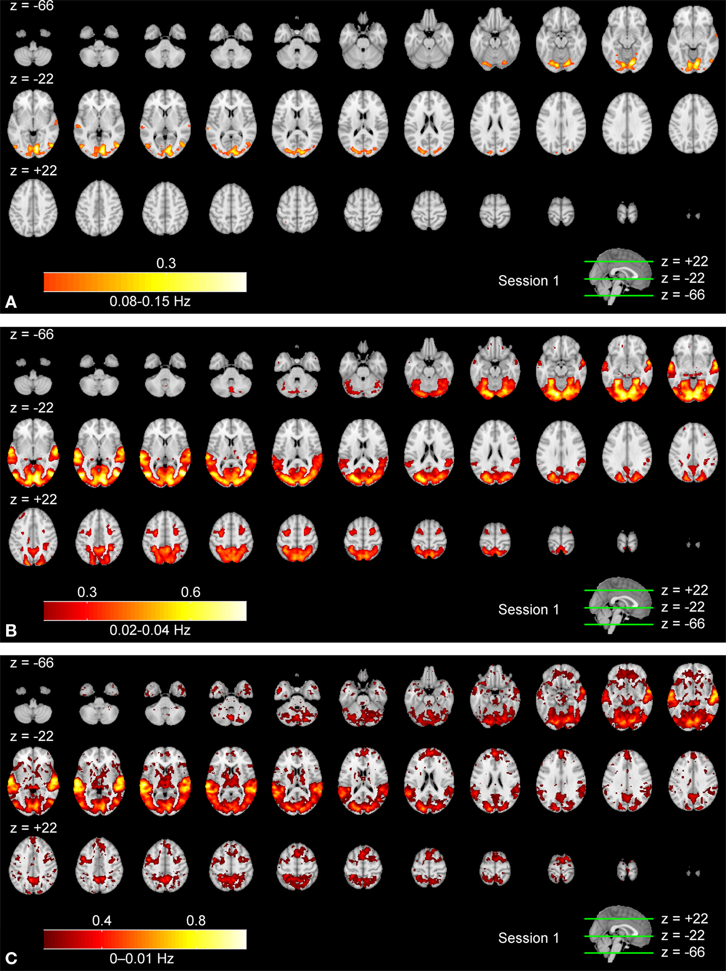
Figure 3. Frequency-specific ISC maps (p < 0. 001, FDR corrected across the whole brain) in the range: (A) 0.07–0.15 Hz, (B) 0.02–0.04 Hz, and (C) 0–0.01 Hz. From top left to bottom right, axial slices are shown from z = −66 to 62 mm (in MNI-coordinates) with 4 mm slice thickness.
Figure 4
shows an indexed multi-frequency ISC map (Eq. 4, p < 0.001, FDR-corrected) across the two scanning sessions. Frequency bands showing strongest ISC are indicated with color coding. The highest frequency band (0.07–0.15 Hz) was omitted because it did not show maximum ISC anywhere in the brain. This visualization scheme provides an overview of the major frequency component showing ISC in different brain areas. This presentation is not suitable for the comparison of the frequency bands, because statistical inference was performed individually within each sub-band.
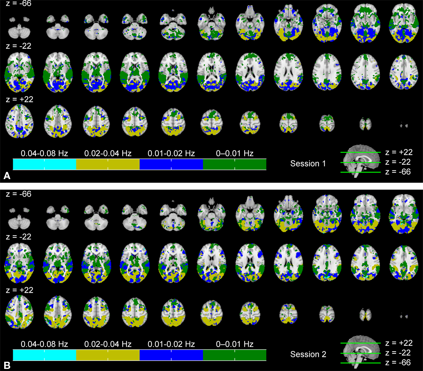
Figure 4. Frequency ranges showing maximum ISC across: (A) the first scanning session, and (B) the second scanning session. From top left to bottom right, axial slices are shown from z = −66 to 62 mm (in MNI-coordinates) with 4 mm slice thickness. The frequency band showing maximum ISC among all the bands is color-coded. The map was thresholded for p < 0.001 (FDR-corrected over the whole brain).
During the first scanning session (Figure 4
A), several occipital areas, including visual areas, occipital fusiform gyrus, and superior parietal lobule, showed maximum ISC in the 0.02–0.04 Hz range (dark yellow). In some areas, such as in lingual gyrus and temporal occipital fusiform cortex, ISC was evident mostly in the 0.01–0.02 Hz range (blue). Some areas, such as occipital pole, temporal occipital fusiform cortex and precuneus cortex showed ISC across a wider frequency range (high ISC in both 0.01–0.02 and 0.02–0.04 Hz bands). ISC in temporal areas was mostly concentrated within the lowest frequency band, i.e., 0–0.01 Hz range (green). Further, several other areas, such as angular gyrus, supramarginal gyrus, and frontal areas (e.g., orbito-frontal cortex) showed maximum ISC mainly in the lowest frequency band. The analysis results across the second scanning session (Figure 4
B) appeared to be qualitatively similar to those obtained across the first scanning session.
Table 2
presents reproducibility analysis (see Eq. 5) results across the two scanning sessions. Results across the full spectrum as well as across each individual frequency sub-band are presented. Reasonably small mean absolute errors were obtained especially across the full spectrum (0–0.15 Hz), and the higher frequency bands (0.07–0.15, 0.04–0.07, and 0.02–0.04 Hz), indicating that ISCs were reasonably well reproducible across the sessions in these frequency bands. Note, however, that there was a gradual increase in q values when moving from higher frequencies towards the lower ones [the highest variability q = 0.049 was obtained in the lowest frequency band (0–0.01 Hz)]. This analysis does not reveal the sources of variability and their respective contribution to the total variability over the two scanning sessions. More advanced methods would be needed to allow conclusions about different sources of variability.
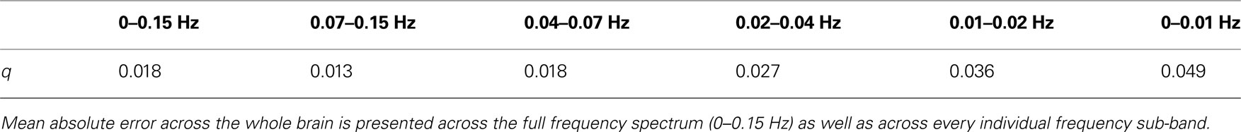
Table 2. Reproducibility of the ISCs across the two scanning sessions.
Frequency Band Comparison
In Figure 5
, three selected sum ZPF maps (Eq. 7), p < 0.05, FWER corrected) are presented to compare ISCs in the lowest frequency band against the ISCs in higher frequency bands. The rest of the results, including the remaining sum ZPF maps of the first scanning session and all the sum ZPF maps of the second scanning session are provided as Supplementary Material. Figure 5
A shows the comparison between the lowest frequency band against the highest frequency band. Warm colors indicate where the low- frequency ISC was significantly greater than the high-frequency ISC. Cold colors show where the ISC in the high-frequency band was significantly greater than the low-frequency ISC. Low- frequency ISC was dominant in temporal cortical areas, and also in some visual and medial frontal cortical areas. Significantly stronger ISCs were not found in the highest compared with the lowest frequency band.
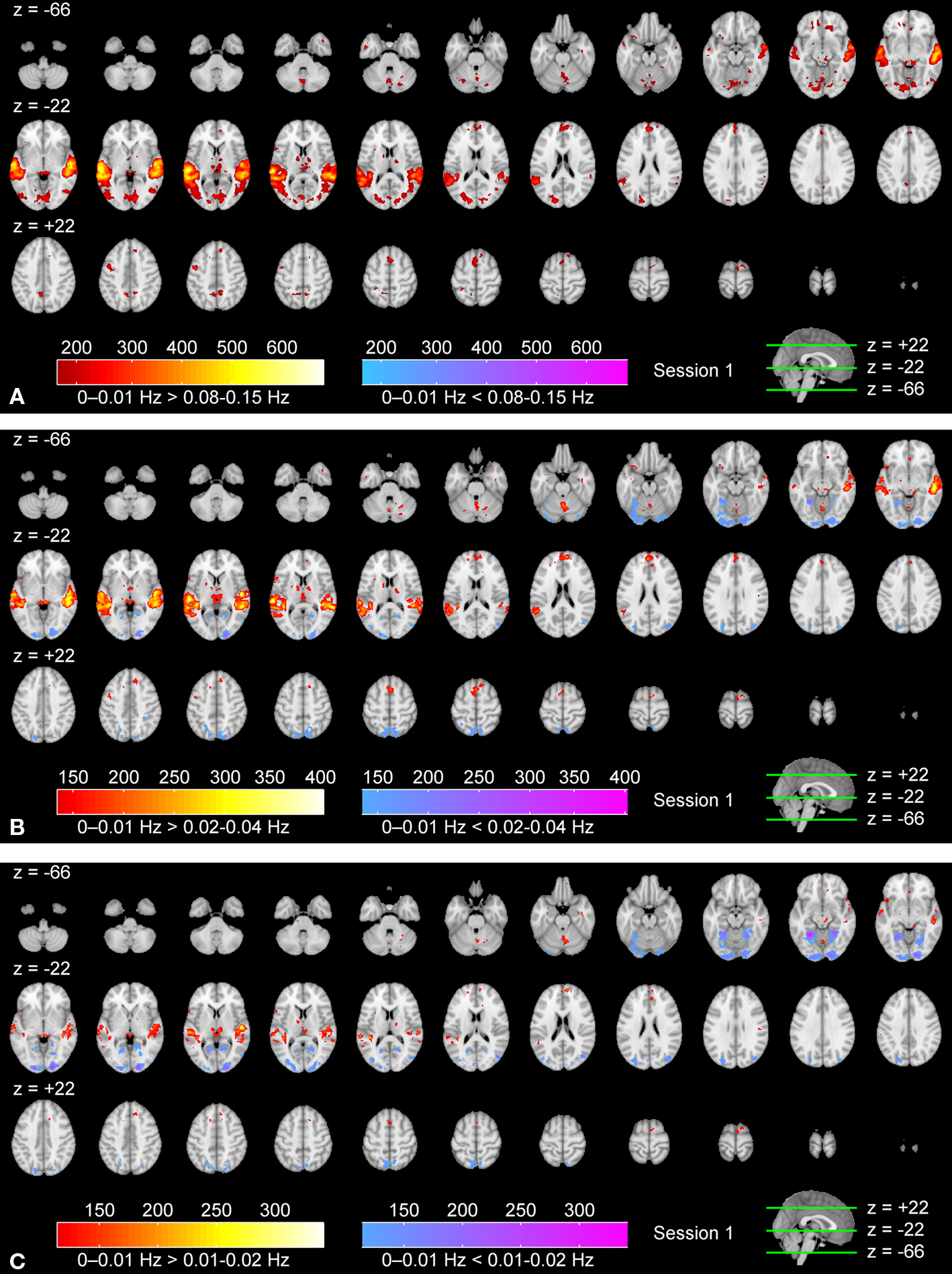
Figure 5. Sum ZPF statistical maps (p < 0. 05, FWER corrected) of the lowest frequency band (0–0.01 Hz) compared with the (A) 0.07–0.15 Hz band, (B) 0.02–0.04 Hz, and (C) 0.01–0.02 Hz band. From top left to bottom right, axial slices from z = −66 to 62 mm (in MNI-coordinates) with 4 mm inter-slice interval are shown. Warm colors show where the ISC in the lowest-frequency band is significantly stronger than in the higher-bands, and cold colors show where the ISC in higher-frequency bands is significantly stronger than the ISC in the lowest-frequency band.
Figure 5
B shows the comparison between the lowest and the middle frequency bands. Again, the low-frequency band showed significantly higher ISC in temporal and frontal areas. In the visual cortical areas, ISC was more dominant in the mid-frequency band compared to the lowest-frequency band. Comparison of the two lowest frequency bands is presented in Figure 5
C. ISCs in the lowest frequency band were not significantly stronger in most brain areas compared to the slightly higher frequency band. This implies, together with the other comparisons, that ISC in frontal and temporal regions was most prominent across the 0–0.02 Hz frequency range. Visual cortex showed significantly higher ISC in the 0.01–0.02 Hz range compared to the lowest frequency band, implying (together with the other comparisons) that visual cortical ISC was concentrated in the 0.01–0.04 Hz range.
Summary
Figure 3
revealed that the frequency range showing significant ISC contracted when moving from lower-order sensory areas towards higher-order cortical areas. In visual cortex, ISC was present across all frequency bands. In temporal areas ISC occurred in all but the highest (0.07–0.15 Hz) frequency band, and frontal cortical ISC was present only in the two lowest frequency bands (0–0.01 and 0.01–0.02 Hz). Further, the combined ISC maps across all frequency bands (Figure 4
), and the results from the specific contrasts between the different frequency bands (Figure 5
), revealed that the strongest ISC component occurs at progressively lower frequencies as one moves from lower-order sensory visual cortical areas towards functionally higher-order cortical areas such as the anterior frontal lobes. However, it should be noted that even in the visual cortical areas, the dominant ISC component occurred at relatively low frequencies (0.01–0.04 Hz). The mean ISC was relatively high in some sensory areas (visual cortical areas in Figure 3
B and temporal areas in Figure 3
C) in contrast to higher order areas, which showed lower ISC values (frontal cortical areas in Figure 3
C). Although this may suggest that neuronal activation in frontal cortical areas was weaker compared to the sensory areas during the movie, the difference may also be explained by inter-individual variability, which might be greater in higher-order areas. Further investigation is required to assess variability of ISC between subjects across different brain areas.
There are a number of possible explanations for the spatial distribution of the ISCs occurring at different frequency bands we found in this study. A recent study, utilizing short silent movie clips, suggested that there is a hierarchy of TRWs in the human brain, with sensory visual cortical areas showing short TRWs, and the TRWs becoming progressively longer as one ascends to functionally higher-order cortical areas (Hasson et al., 2008c
). While a more limited range of cortical areas was found to be activated than in the present study, perhaps due to the unimodal nature of the stimulus and the fact that the movie clips were relatively short, the frontal and temporal cortical areas that were significantly activated (frontal eye field, posterior lateral sulcus, and temporal–parietal junction) showed the longest TRWs. Thus, it is possible that the present low-frequency ISCs in frontal and temporal areas is explained by longer TRWs in these areas. On the other hand, visual features of the movie that sensory cortical areas process occur at higher frequencies than, for instance, interpersonal communication and/or development of social relationships between movie characters that the temporal and prefrontal cortical areas should be more sensitive to (see Carrington and Bailey, 2009
). However, further investigations are required to find out whether and how the low frequency frontal cortical ISCs/BOLD fluctuations specifically relate to the stimulus.
Visual cortex showed ISC extensively across all frequency bands, possibly reflecting different phenomena. For example, high frequency ISC component can be related to the TRWs and low frequency component may be partially induced by modulatory and top-down inputs (Monto et al., 2008
). The frequency components can also reflect other stimuli related phenomena such as temporal correlations within stimuli itself.
Conclusion
We extended ISC analysis to frequency domain by combining wavelet analysis to non-parametric permutation methods for making group-level voxel-wise statistical inferences about frequency-band specific ISC. Computationally intensive non-parametric methods were necessary for statistical inference because of the dependency among subject pair-wise correlation coefficients that were averaged to yield the ISC-statistics. Our results suggest that several regions within the frontal and temporal lobes show ISC predominantly at low frequency bands, whereas visual cortical areas exhibit ISC also at higher frequencies. It is possible that these findings relate to recent observations of a cortical hierarchy of TRWs, or that the types of events that the temporal and prefrontal cortical areas are processing (e.g., social interactions) occur over longer time-scales than the stimulus features processed in the visual areas. Software tools to perform frequency-specific ISC analysis, together with the visualization software, are made available as open source Matlab code at Supplementary Material.
The authors declare that the research was conducted in the absence of any commercial or financial relationships that could be construed as a potential conflict of interest.
This work was supported by the Academy of Finland, (grant number 130275 and 129657, Finnish Programme for Centres of Excellence in Research 2006–2011), the aivoAALTO project funding of the Aalto University, the University Alliance Finland Research Cluster of Excellence STATCORE and Tampere Graduate School in Information Science and Engineering (TISE).
The Supplementary Material for this article can be found online at
http://sites.google.com/site/frequencyspecificisc/
http://sites.google.com/site/frequencyspecificisc/
Smith, S. M., Jenkinson, M., Woolrich, M. W., Beckmann, C. F., Behrens, T. E. J., Johansen-Berg, H., Bannister, P. R., De Luca, M., Drobnjak, I., Flitney, D. E., Niazy, R. M., Saunders, J., Vickers, J., Zhang, Y., De Stefano, N., Brady, J. M., and Matthews, P. M. (2004). Advances in functional and structural MR image analysis and implementation as FSL. Neuroimage 23, 208–219.