1
Adaptive Behaviour Research Group, Department of Psychology, University of Sheffield, Sheffield, UK
2
Department of Biophysics, KFKI Research Institute for Particle and Nuclear Physics, Hungarian Academy of Sciences, Budapest, Hungary
Computational neuroscience is increasingly moving beyond modeling individual neurons or neural systems to consider the integration of multiple models, often constructed by different research groups. We report on our preliminary technical integration of recent hippocampal formation, basal ganglia and physical environment models, together with visualisation tools, as a case study in the use of Python across the modelling tool-chain. We do not present new modeling results here. The architecture incorporates leaky-integrator and rate-coded neurons, a 3D environment with collision detection and tactile sensors, 3D graphics and 2D plots. We found Python to be a flexible platform, offering a significant reduction in development time, without a corresponding significant increase in execution time. We illustrate this by implementing a part of the model in various alternative languages and coding styles, and comparing their execution times. For very large-scale system integration, communication with other languages and parallel execution may be required, which we demonstrate using the BRAHMS framework’s Python bindings.
As computational resources inexorably grow, computational neuroscience is increasingly moving beyond modeling individual neurons or neural systems to consider the integration of multiple models, often constructed by different research groups. At the software level there is a drive towards interoperability of simulators at both model specification (Goddard et al., 2001
) and run-time stages (Cannon et al., 2007
). However, these efforts have concentrated on creating small networks of different multi-compartment models (Gleeson et al., 2007
), or large networks of different single-compartment spiking neuron models (Cannon et al., 2007
).
Our focus here is on a third strand that can take advantage of growth in computing power: the integration of multiple neural models that form components of a brain-wide system, and the testing of that integrated model in an embodied form. Embodiment often takes the form of a robot and a test environment, whether simulated or real. Requiring the neural models to generate appropriate behavioural output using only inputs available in the environment is a strong test of the proposed computations of that neural system (Humphries et al., 2005
; Prescott et al., 2006
). In such large simulations, development time is as much an issue as computation time – to implement and test the models, construct simulated environments, implement realistic sensors, and so on. This paper shows how Python provides an excellent solution to both development and computation time problems; we also discuss how Python can work with platforms designed for such large-scale integration (Mitchinson et al., 2008
).
As a case study, we report on our preliminary integration of recent hippocampal formation and basal ganglia models, both proposed components of the neural system for spatial navigation (Redish and Touretzky, 1997
). The hippocampal formation’s role in spatial navigation is not controversial: “place” cells within
CA1/CA3 encode position in space (O’Keefe and Conway, 1978
; Wiener, 1996
); “grid”-cells in entorhinal cortex (EC) provide metric information for path-integration via a tessellating rhomboid pattern (Hafting et al., 2005
; McNaughton et al., 2006
); and hippocampal lesions impair (but not necessarily abolish) rats’ abilities to navigate in open environments (Whishaw, 1998
). The basal ganglia’s main input nucleus – the striatum – is a major target of hippocampal formation output, and also appears necessary for unimpaired spatial navigation: lesioning the connecting fibres impairs accurate navigation in open environments (see e.g. Devan et al., 1996
; Gorny et al., 2002
; Whishaw et al., 1995
), and blocking plasticity in the region of striatum targeted by hippocampal fibres prevents acquisition of paths to targets (Sargolini et al., 2003
; Smith-Roe et al., 1999
).
A recurring theme in the basal ganglia literature is that they form a selection mechanism for motor programs (Hikosaka et al., 2000
; Mink and Thach, 1993
) or, more generally, for “actions” (Redgrave et al., 1999
). Thus, the specific hypothesis underlying our integrated model is that the basal ganglia select movement direction based on current spatial position provided by the hippocampal formation input.
The system described below is a preliminary technical integration of the action-selecting basal ganglia model of Gurney et al. (2001a
,b)
with the hippocampal navigation model of Ujfalussy et al. (2008)
. The basal ganglia model may be used to select between any types of action, but simple predefined saliencies between two target locations are currently used. The hippocampus model may run using any form of sensory input: at present we use visual input, but report on the implementation of physical simulation of tactile whisker-like sensors as an example of developing advanced sensors in Python, which could form a further input in future. Neither the inputs to the models or the placeholder function connecting them are intended to be biologically realistic at this stage. The neural models control a mobile rat-like robot in a standard plus-maze environment with external landmarks, all implemented in a 3D simulator built using existing Python modules. The purpose of this paper is to illustrate a complete neural and physical simulation system, detailing the specific libraries and packages in the tool-chain that were found useful, and not to make any new claims about the biological models. We hope that it will provide a guide for others who wish to implement similar systems, as it can be difficult for newcomers to select the best tools from the plethora of open-source Python extensions.
We are updating prior models of hippocampal formation-basal ganglia interactions (Arleo and Gerstner, 2000
; Chavarriaga et al., 2005
) by including the entire basal ganglia circuit and by using a grid-cell driven model of hippocampus. In addition, prior models assumed a direct, modifiable, projection from place cells to the striatum (Arleo and Gerstner, 2000
; Chavarriaga et al., 2005
). However, such a projection, if it exists, is minor compared to input from other regions of the hippocampal formation, particularly the subiculum, suggesting further stages of processing between the basic representation of position and the striatum (see e.g. Groenewegen et al., 1999
; van Groen and Wyss, 1990
). In the current integrated system, we provide a simple spatial decoding scheme as a proxy for detailed models of the intervening structures to follow. We do not here present new results from the individual models (Gurney et al., 2001a
,b
; Ujfalussy et al., 2008
), but report on systems integration at a technical level using Python and BRAHMS.
Basal Ganglia
The basal ganglia are a group of inter-connected subcortical nuclei, which receive massive convergent input from most regions of cortex, and output to targets in the thalamus and brainstem (Bolam et al., 2000
). We have previously shown how this combination of inputs, outputs, and internal circuitry implements a neural substrate for a selection mechanism (Gurney et al., 2001a
,b
, 2004
; Humphries and Gurney, 2002
; Humphries et al., 2006
; Prescott et al., 2006
). Figure 1
illustrates the macro- and micro-architecture of the basal ganglia, highlighting three key ideas underlying the selection hypothesis: that the projections between the neural populations form a series of parallel loops – channels – running through the basal ganglia from input to output stages (Alexander and Crutcher, 1990
); that the total activity from cortical sources converging at each channel of the striatum encodes the salience of the action represented by that channel; and that the selection of an action is signalled by a process of disinhibition – the selective removal of tonic inhibition from cells in the basal ganglia’s target regions that encode the action (Chevalier and Deniau, 1990
).
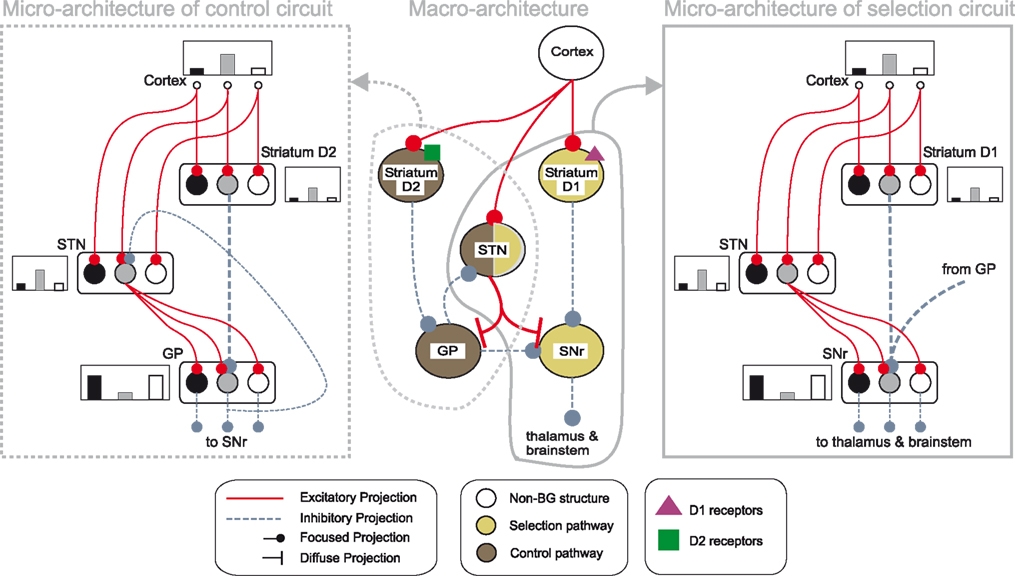
Figure 1. Architecture of the basal ganglia model. The main circuit (centre) can be decomposed into two copies of an off-centre, on-surround network: a selection pathway (right) and a control pathway (left). Three parallel loops – channels – are shown in both pathways, with example activity levels in the bar charts to illustrate the relative contributions of the nuclei (the three channels are colour-coded black/grey/white, corresponding to the example bar charts). Note that, for clarity, full connectivity is only shown for the second channel. Briefly, the selection mechanism works as follows. Constant inhibitory output from substantia nigra pars reticulata (SNr) provides an “off” signal to its widespread targets in the thalamus and brainstem. Cortical inputs representing competing saliences are organised in separate channels (groups of co-active cortical neurons), which project to corresponding populations in striatum and STN. In the selection circuit, the balance of focussed (one-to-one) inhibition from striatum and diffuse (one-to-many) excitation from STN results in the most salient input suppressing the inhibitory output from SNr on that channel, signalling “on” to that SNr channel’s targets. In the control circuit, a similar overlap of projections to GP exists, but the feedback from GP to the STN acts as a self-regulating mechanism for the activity in STN, which ensures that overall basal ganglia activity remains within operational limits as more and more channels become active. For quantitative demonstrations of this model, see Gurney et al. (2001b
, 2004) and Humphries et al. (2006)
.
We use here the population-level implementation of this model from Gurney et al. (2001b)
. The average activity of all neurons comprising a channel in a population is represented by a single unit that changes according to

where τ is a time constant and u is summed, weighted input. We use τ = 40 ms. The normalised firing rate y of the unit is given by a piecewise linear output function
The following describes net input ui and output yi for the ith channel of each structure, with n channels in total. Net input is computed from the outputs of the other structures, except cortical input ci to channel i of striatum and subthalamic nucleus (STN). The striatum is divided into two populations, one of cells with the D1-type dopamine receptor, and one of cells with the D2-type dopamine receptor. Many converging lines of evidence from electrophysiology, mRNA transcription, and lesion studies suggest a functional split between D1- and D2-dominant projection neurons and, further, that the D1-dominant neurons project to SNr, and the D2-dominant neurons project to globus pallidus (GP; Gerfen and Wilson, 1996
; Surmeier et al., 2007
).
Activation of these receptors has opposite effects on striatal input: D1 activation increases the efficacy of the input; D2 activation decreases the efficacy of the input (see Gurney et al., 2001b
, for full details). Let the level of tonic dopamine be λ: then the increase in synaptic efficacy due to D1 receptor activation is given by (1 + λ); the decrease in synaptic efficacy due to D2 receptor activation is given by (1 − λ). Normal dopamine levels were indicated by λ = 0.2, and dopamine-depletion by λ = 0, following previous work (Gurney et al., 2001b
; Humphries and Gurney, 2002
). The full model is thus given by:
Full details for the chosen constants can be found in (Gurney et al., 2001a
), and are summarised here. Thresholds for striatal output were set ε > 0 so that a large positive input would be required for any output from these neurons, modelling the large input required to push the striatal projection neuron into its firing-ready “up-state” (Gerfen and Wilson, 1996
). The STN, SNr, and GP all had ε < 0, as each of these has tonic output at rest (Bolam et al., 2000
). Non-unity weights (0.3,0.9) on inputs were set to be within analytically-derived bounds for stable operation of the model (Gurney et al., 2001a
).
We used forward Euler to simulate this system for a two-channel model, with the same time-step of 10 ms as was used for the discrete equations of the hippocampus model (see below).
The model was implemented in Python using an object-oriented hierarchy. Neuron objects contain Dendrite objects, which store modulated and unmodulated weights, and references to parent neurons. Neurons also store their parameters (ε,τ,s) (where s is the sign of dopamine action) and state (u,a,y). The neuron class contains methods to apply dopamine modulation and determine the unit’s output. A Population class groups units together, and contains methods to instantiate sets of one-to-one (e.g. GP→SNr) or diffuse (e.g. STN→SNr) links to other Populations. These methods automatically construct Dendrite objects and update references.
We have found Python’s default and named arguments to be especially useful in this type of modeling. Neurons may be given many default parameter values which remain invisible in the user-level code unless specifically overridden. For example, the sign s of dopamine action is assumed to be zero (meaning no effect) unless an easy-to-read named parameter is passed:
Hippocampal Formation Model
The hippocampal formation comprises the EC, dentate gyrus (DG), fields CA3 and CA1 of the hippocampus proper, and the subiculum. These form a feed-forward loop of connections that starts and ends in the EC. Though all structures are thought to contribute, the hippocampal model of Ujfalussy et al. (2008)
instantiates just the minimum putatively required for the hippocampal formation to act as a memory store (following Treeves and Rolls, 1994
); for spatial navigation, the memory formed is considered the place code created by the place cells. Figure 2
shows the basic structure, formed by just the EC, DG, and CA3.
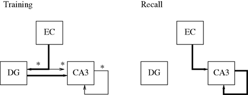
Figure 2. Basic structure of the hippocampal model. Different connections are active during learning and recall modes. Learning is performed on the asterisked connections only. Thin lines indicate connections which do not drive their targets, but perform learning only.
Following previous models (e.g. Treeves and Rolls, 1994
), the model of Ujfalussy et al. (2008)
makes three key assumptions. First, the DG region is a preprocessing stage for CA3, acting as a competitive network that creates a sparse and clustered code of the pre-synaptic EC input, which – similarly to other neocortical regions – realises a denser representation. This sparse, orthogonal code is in turn used as a teaching signal for the CA3 region. Second, the CA3 region acts as an auto-association memory, which stores memory traces in its extensive recurrent local collaterals for later retrieval. Third, many previous hippocampal models (Arleo and Gerstner, 2000
; Rolls, 1995
; Treeves and Rolls, 1994
) assume that the hippocampus operates in two distinct modes during learning and retrieval, which are also incorporated into the present model. As in these models, switching between the two modes is performed manually (contrary to models such as Hasselmo et al. (1995
, 1996)
which explicitly address the separation between learning and recall). Figure 2
shows the connections that change between the modes.
Entorhinal cortex
Grid cells in EC are modeled as having firing rates that are functions of the agent’s actual physical position r = (x,y) in the simulated environment. Grid cells each have two parameters, determining the phase and scale of their receptive fields. The output of the i,jth grid cell is
where si and θj are the ith scale factor and jth phase shift respectively, and  are unit vectors at 60° from each other. We used an ordered set of scale factors from 0.5 to 2.5 in steps of 0.5, and an ordered set of phases from 0 to π in steps of π/5; i and j are indices into these sets. Figure 3
shows that Eq. 13 produces receptive fields with the characteristic rhomboid or “double triangle” tesselation of grid cells (Hafting et al., 2005
).
are unit vectors at 60° from each other. We used an ordered set of scale factors from 0.5 to 2.5 in steps of 0.5, and an ordered set of phases from 0 to π in steps of π/5; i and j are indices into these sets. Figure 3
shows that Eq. 13 produces receptive fields with the characteristic rhomboid or “double triangle” tesselation of grid cells (Hafting et al., 2005
).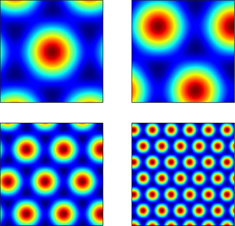
Figure 3. Grid cell receptive fields from the model, over physical 2D space. These are plotted with Pylab’s Matlab-style
imagesc command.The EC relays input from several cortical areas (Marr, 1971
) to the hippocampal formation, and is thus often treated (e.g. Rolls, 1995
; Rolls et al., 2006
), as in the present model, as the input source for all sensory information. Thus, as well as comprising a large population of grid cells, EC is modelled with an additional population of sensory cells. We use 100 visual cells, whose activations are set by 10 × 10 grayscale images.
Dentate gyrus
The DG is thought to perform a principal-components-like dimensionality reduction of input from the EC (Lorincz, 1998
). Writing wij for weights on inputs yi, the jth DG unit’s neural activation is given by

where the sum is taken over all EC inputs. Output firing rates {yj} are given by a m-best function {yj} = F{aj} which preserves the m largest activations, linearly re-maps them to the interval [0,1], and sets the others to zero.
During the training phase only, every EC → DG weight is updated at each time-step using the standard Hebbian learning rule,

where α is the learning rate, and again j represents the DG cell population and i represents the afferent EC population.
CA3 place cells
CA3 functions differently during training and recall. During training, CA3 is driven only by input from DG; hence unit activity is updated according to Eq. 14 with j representing the CA3 cell population and i representing the afferent DG population. CA3 output is computed from these activations with the same m-best function used for the DG output.
Despite being driven by DG only, no learning is performed on this connection. Instead, learning is performed on the otherwise dormant EC→CA3 and CA3→CA3 pathways. EC→CA3 weights are altered by Eq. 15, where yi is EC output, and yj is CA3 output. Following Rolls (1995)
, each recurrent CA3→CA3 weight is altered by the gated Hebbian rule,

where β sets the “forgetting rate”, and i and j now both refer to cells within the CA3 population.
During the recall phase, the EC input is used to initiate retrieval of a stored memory pattern. First, the activation of CA3 units is computed from the EC inputs only, using Eq. 14 with j representing the CA3 cell population and i representing the afferent EC population; their output is then computed using the m-best function. Second, this initial output vector was used as the cue to retrieve the memory trace in the CA3 autoassociative network. The activity of the kth CA3 unit is then the weighted sum of total output from the EC and the recurrent connections

with CA3 output yk again computed by applying the m-best function. Activation (Eq. 17) and output calculations of the CA3 units were iterated I times to bring the CA3 close to an attractor state as in Hopfield-style networks (Hopfield, 1984
).
We used eight DG cells and 30 CA3 cells with: learning rate α = 0.05, forgetting rate β = 0.00002, sparsity m = 20 and I = 5 recurrent iterations.
Implementation in Python
The hippocampal model uses simple rate-coded units and linear weights, in contrast to the basal ganglia’s leaky integrators. For this reason the population activations and firing rates are amenable to fast implementation as vectors rather than as attributes of individual objects. Multiplication of population firing rates by weight matrices may then be performed by matrix algebra. This style of programming is common in Matlab, and may be performed in Python using the Numpy library
1
. Numpy emulates much of Matlab’s matrix syntax, including notation for slicing matrices (e.g.
A = M[:,1:5]), addressing (M[2,3] = 4) and performing operations such as element-wise addition (B = A + 1) as well as matrix algebra (C = dot(A,B)).We have also made use of two further libraries: SciPy
2
provides a library of higher-level mathematical functions similar to Matlab’s toolboxes; and Pylab
3
provides interactive plotting commands. For example, Figures 3 and 4
were plotted using Pylab. Pylab emulates many of Matlab’s graphics commands including 2D and 3D graphs, and image viewers. The Matlab application programmer interfaces (APIs) are replicated almost literally, using the same function names and argument conventions where possible, such as
clf, plot and imagesc.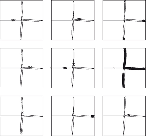
Figure 4. Receptive fields for nine CA3 place cells, superimposed on the robot’s path around the plus maze. Crosses show locations where cells firing rates are in the top 5% of their activity throughout the path. Plotting was performed with Pylab’s
plot command, which has similar syntax to Matlab.Training
Training of the EC→DG, EC→CA3 and CA3→CA3 weights was performed over five epochs. Weights were initialised to random real values from a uniform distribution ranging from 0 to 1. Grid and visual cell input data was collected from a simulated robot moving to a sequence of pre-determined points in a plus-maze environment (see “Building and Using the 3D Simulator” for simulator details). The robot enters the maze from the open arm, then visits each of the other arms in turn and comes to rest at the center. About 1,500 data points were sampled during this motion. After training, Python’s standard cPickle library provided a simple way to serialise and save the trained Hippocampus object, using only the following code:
The effect of training the hippocampus model with the grid cell and visual input was to generate place fields in CA3, such as those shown in Figure 4
, which shows the locations of strongest firing for nine of the 30 CA3 cells, superimposed on the robot’s path. Of the 30 cells simulated, 11 responded to single places, 13 to two or more places, and 6 were silent at all places (where a “single” place is defined as a contiguous series of strong activations).
Decoding Place
We used a placeholder function for decoding hippocampal place representations into striatal input, as a proxy for detailed models of the intervening structures (e.g. CA1, subiculum) to follow. A simple linear regression was used to find a linear mapping from the vector of place cell activations to the Cartesian (x,y) spatial positions. SciPy provides such regression in its linear algebra sub-package (function
linalg.lstsq).The Plus-Maze Environment
We used Python to construct a plus-maze environment in which to test our current and future forms of the integrated basal ganglia-hippocampus model. The plus-maze environment was chosen as it is widely used for neural recording studies that probe the roles of striatum, hippocampus, and their interactions in spatial tasks (Albertin et al., 2000
; Khamassi, 2007
; Mulder et al., 2004
; Tabuchi et al., 2000
, 2003
). Following these studies, the simulated plus-maze comprised a symmetric arrangement of walled arms, and two extra-mazecues (Figure 5
).
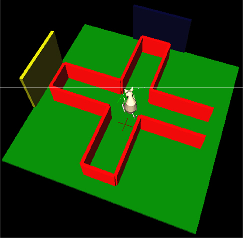
Figure 5. The simulated plus-maze environment. The hippocampus reports the current estimated location, shown by the cross on the floor. When this estimate is close to the center of the plus-maze, the basal ganglia is consulted for an action to turn. 3D physical simulation and visualisation uses PyODE and Pivy.
The neural model was used to control the “ICEAsim” simulated robot, a differential wheels robot in a rat-like form, created by Cyberbotics (Lausanne) for the ICEA project
4
. ICEAsim was initially created under Cyberbotics’ Webots simulator (Michel, 2004
), but was readily imported into a Python simulation via the standard VRML format. Wheel commands are sent via a higher-level (and non-biological) function which takes as input a requested target location to which to move. Our implementation of ICEAsim added two whisker sensors, which output the angle and curvature at their bases for use in tactile perception algorithms (see “Python Physics Implementation” and “Comparison to PyRobotics”). We added realistic whisker-like sensors as the basis for future studies: while rats can successfully navigate in the dark, and corresponding place fields are formed in the hippocampal formation, this has been attributed entirely to idiothetic (self-motion) cues (Quirk et al., 1990
; Rossier et al., 2000
); surprisingly little attention has been paid to the potential role of rats’ whiskers in constructing spatial maps in the dark.
For the purposes of this paper, we used a simple task and a placeholder function to test that the models were correctly implemented and technically integrated. After hippocampal training (a separate task, not involving basal ganglia), the robot was simply required to successfully navigate to the end of a maze arm, starting from the entrance of the maze. The basal ganglia model received input saliences {c1,c2} on two channels, corresponding to two actions (“go to left arm” and “go to right arm”), and which – in this preliminary system – were assigned predefined time series. The placeholder function monitored the hippocampal position estimate, and when this estimate was close to the center of the maze, the action corresponding to the basal ganglia output channel (in SNr) with minimum value was selected and executed to completion. A “go to left arm” or “go to right arm” routine is called, which uses hippocampal output to estimate the required path to follow and sets the robot’s differential wheel speeds accordingly. Figure 5
illustrates the simulated robot’s behaviour: video of the robot’s movement, and corresponding activity in the integrated neural models, are available as Supplementary Material. Future biological models of basal ganglia-hippocampus interactions may of course replace the predefined time series and placeholder function with more complex and ongoing interactions between the models, using the technical integration framework presented here.
Python Physics Implementation
To simulate tactile whisker sensors requires realistic physics modeling, as the precise bending (Birdwell et al., 2007
), vibration (Ueno and Kaneko, 1994
) and other dynamics (Ritt et al., 2006
) of whiskers are crucial in making inferences from touch. The Open Dynamics Engine (ODE) is an excellent open-source (BSD license) physics engine, and we use the PyODE wrapper (pyode.sourceforge.net) to use it from Python. ODE provides primitive objects such as cubes, spheres and cylinders, which may be combined and transformed to produce objects such as the walls of the plus-maze and the parts of the robot. PyODE wraps all the major ODE functions for shapes, kinematics and collision handling, and provides access to ODE’s standard set of flexible joints. We use the latter to construct rotating wheels, and whiskers. The whiskers are modelled as a series of spherical or cylindrical segments, connected by joints with rotational Hooke’s law springs. ODE handles the constraint forces required to keep joints together automatically; however very small time steps (and hence long simulation times) are needed when the number of segments is above three. For example with three segments per whisker the simulation requires about 3 min to run stably on a 1.6-GHz machine; with four segments it requires about 10 min.
Visualisation
3D visualisation is important in robotics simulation, both to ensure that the simulation is behaving as intended, and also to provide realistic visual input to robot sensors, for processing by neural models.
OpenGL is a standard 3D graphics API
5
, and is implemented by the free software Mesa and by many hardware-specific graphics drivers. OpenGL provides low-level graphics commands to draw lines, triangles and polygons, and position lights and cameras. The OpenGL API is wrapped in Python by pyOpenGL (pyopengl.sourceforge.net).
Higher-level graphics commands – such as drawing cubes, cylinders and cones using scene graphs – are provided by the OpenInventor API, implemented by the free software Coin
6
. Coin has been wrapped for Python by the Pivy binding
7
(Fahmy, 2006
) which we use here. Pivy allows raw pyOpenGL commands to be mixed into its higher-level structures where necessary.
To simulate vision (for input to the hippocampus model) we read back images from simulated cameras attached to the robot. Pivy wraps Coin’s
SoOffScreenRenderer function to perform this task. (Modelers are advised that use of this function may be incompatible with the use of direct rendering on some graphics hardware. Disabling direct rendering solves this problem but reduces execution speed.) If graphical output is required in video form only – such as for presentation but not as data for neural models – the free program Yukon
8
is able to export OpenGL graphics to .avi movies, whose frame rate and resolution may be edited with the free Avifix program
9
.In addition to the main 3D representation of the physical world, it is often useful to attach additional graphical monitors to show the internal state of the neural models in real-time. Pivy – like Coin – takes control of program flow, calling back user functions to draw and update the world. When multiple displays are required – or when handing over control is too intrusive – it is useful to instantiate several processes running Pivy. We use the Python Remote Objects package (PyRo
10
) to handle communication between such processes. PyRo allows an object from one process to appear on another as if it was resident there, allowing function to be called and data to be passed easily. PyRo processes communicate via TCP/IP so the monitors may run on different machines to the main simulation. Figure 6
shows a screen-shot of the state visualisation tool we built for the integrated basal ganglia-hippocampus model.
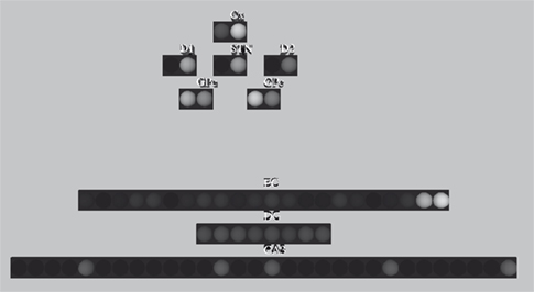
Figure 6. Real-time graphical neuron monitor, showing basal ganglia and hippocampus model populations. The monitor runs remotely from the simulation over TCP/IP using Pyro, and displays graphics using Pivy.
Comparison to Pyrobotics
Our simulation is constructed using Python wrappers for ODE and OpenGL. An alternative approach to simulation would be to use the higher-level Player interface and Gazebo simulator
11
which are available though the PyRobotics
12
integrated robotics simulator. PyRobotics allows worlds and robots to be built from standard components using XML specification, and controllers written in Python. This approach is recommended for simulations requiring standard physics, but our use of the lower-level APIs was determined by the need to write custom physics code for the whisker sensors. Whiskers are difficult to model and coding with ODE directly allows finer control over the contacts and forces that are simulated than would be available in a higher-level simulator. Our custom simulations are not intended to be an integrated robotics simulator, but they serve as an example of lower-level PyODE and Pivy simulation.
Python is often thought of as being a “slow language” and if this is the case then it would be a barrier to its use in large scale, computationally-intensive neural simulations. However, various libraries and programming styles exist that can improve performance. We investigated a variety of these to evaluate Python’s suitability for large simulations. We chose execution of the previous basal ganglia model alone as a benchmark representative of many neural simulation tasks, and used a model with 100 channels running over 1,000 time steps to provide a sizable task requiring time of the order of seconds. Neural models are commonly implemented in high-level Matlab code (and its open-source equivalent, Octave), or in low-level C code. C code allows and requires the user to perform their own memory management, leading to greater development time but often faster running times. We re-implemented the basal ganglia model in these languages, writing the fastest code our skills allowed.
In addition to the object-oriented Python model described earlier, we also re-implemented Python models using the Numpy, Pyrex and Weave libraries. As described above, Numpy provides Matlab-like data structures, operations and syntax, to the extent that the Matlab program can be ported to Numpy with only minor syntactic modifications. Pyrex
13
is a Python-like language for writing Python extension modules, which provides C-like manual typing and data structures. As with C, Pyrex increases development time by adding work to the programmer’s load, but may increase execution time as a result. Programming Pyrex is conceptually similar to writing C programs, but using a Python-like syntax and allowing very simple integration into pure Python code. Weave (part of SciPy) allows inline C code to be embedded directly into Python files, and its “converters” library automates data type conversion between languages. We implemented inline Weave code within the body of the main Numpy simulation loop.
Another way to improve Python speed is to use more advanced compilers and virtual machines. There is much current research into such tools but a popular system is Psyco
14
. We used Psyco to run the pure Python, object-oriented model (it has negligible effect on Numpy code, in which most of the computation is performed by external numerical C libraries).
Table 1
shows the average execution times for the above implementations (and a BRAHMS version discussed below). Execution was performed on a 1.6 GHz, 1.5 GB Ubuntu system and time averages were taken over five runs. No calls were made to platform-specific BLAS or random-number generator libraries within the simulation loops (such calls are not required or useful in implementing the basal ganglia model’s equations). It can be seen that for the Matlab and C-like programming styles (i.e. Numpy and Pyrex respectively) Python is about four times slower than the non-Python alternative. Weave is only a fraction slower than raw C, the overhead being due to type conversions. The object-oriented version has a much larger run-time – as expected of this style of programming – and the time is reduced by about 25% using Psyco.
These results suggest that Python is not inherently “slow” – a factor of four is not large in such comparisons – though it can be used to write slow but conceptually meaningful, human-readable, object-oriented code if desired. Alternatively, if human comprehension is less important, then Matlab-like and C-like programming styles can be used to regain speed. In most cases it is desirable to work on an easily comprehendible “reference implementation” of a model at first, then develop a faster implementation once the research is complete. Python eases this often difficult transition as Numpy, Weave and Pyrex commands may be gradually mixed into and replace the research code: the more traditional replacement of Matlab by C programs requires a complete rewrite from scratch.
The above has considered architectural and computational features of Python and its associated libraries that are useful in embodied neural modeling. However these are not the only criteria for choosing a language for development: at least as important are the more subjective aspects of the system during development and debugging. Here we offer our experiences of hands-on development of the neural and physical models.
We have found that Python supports a wide range of coding styles. In particular, it is possible to code almost literal line-by-line translations of Matlab programs by making heavy use of Numpy’s matrices and Pylab’s plotting facilities. A key feature is the ability to use interpreted Python from a command line, enabling Matlab-like exploitation of data, testing of functions, and calculator-style calculations. There is typically a little more keyboard typing than when using Matlab. Throughout we have drawn explicit parallels between using Python and Matlab, as Matlab (or Octave) is often the preferred choice for rapid model development and analysis.
Python’s class system allows Java-like object-oriented construction of dendrites, neurons and populations. Stylistically its use is similar to Java, or C++ with passing by reference. We have found it a natural but relatively slow-execution way to model neural systems.
The physical and neural simulation, with OpenGL interface, runs at comparable speed to commercial robotics simulators such as Webots (Cyberbotics, Lausanne). We have found development time to be much improved over C++, and comparable with Matlab. However Python gives more versatility than Matlab, allowing easy integration with many open-source libraries and the underlying operating system. Our development has used Emacs with its Python mode. In particular, this integrates with the Python debugger, pdb, to allow visual stepping through code and command-line interaction as in Matlab. This type of interaction can be especially important in neural and AI programs, whose states and interactions can become very complex in unpredicted ways.
All of the components discussed above (basal ganglia, hippocampus, 3D simulator) were implemented as stateful functions in Python. Thus, integrating them into a computational system was straightforward, by writing a simple Python “main” function that called these objects in turn to progress them through time. Such an approach to integration is effective, so long as there is no requirement for integration across more complex boundaries. One example of a more complex boundary is cross-language: integrating between functions written in Python, C, Java, or Matlab, for instance, is not generally straightforward. Whilst Python might be a suitable language for large portions of a development, bottleneck computations may benefit from being recoded in a lower-level language such as C. Besides, contributing authors may not all share competence and/or enthusiasm for Python development.
Other obstacles to integration include different component authors, particularly in different groups. This can be problematic since different authors tend to design different interfaces for their components and, in the world of research, rarely have time to properly document these interfaces. Integrating through time – that is, using code written some years ago with code written today – can throw up the same problems as integrating across authors, particularly if documentation is lacking. Cross-platform integration is sometimes necessary, particularly as emphasis shifts to high-performance or embedded computing, and this is far from trivial.
As such multi-module eclectic models become prevalent, and with growing interest in widely varying use cases (high-performance, desktop, embedded), a general solution to the integration problem is urgently required. One such solution is the BRAHMS Modular Execution Framework (brahms.sourceforge.net; Mitchinson et al., 2008
). BRAHMS consists of a supervisor, which is analogous to the simple Python “main” function mentioned above, a fixed supervisor interface against which software components can be developed (currently available in C, C++, Matlab and Python), and a user-extensible set of data types for passing data between software components (forming the inter-process interface). Components need not agree between themselves on implementation: they need only conform to these two interfaces provided and made public by the framework. A BRAHMS system, constructed from processes authored as described below, can be parallelised across computer cores sharing memory or connected by an MPI layer or LAN; alternatively, it can be run on an embedded system, since BRAHMS is lightweight. Here we describe the BRAMHS Python language binding.
A Brahms Process in Python
The current BRAHMS Python binding (called “1262”) requires that the process be implemented as a function; this function is rendered stateful by passing in and out a reference to a dictionary object, called persist. The function is a handler for framework events, so its body consists of a switch block on the event type. The 1262 template provided with BRAHMS handles four events.
The first, (
EVENT_MODULE_INIT), returns information about the process to the framework, and is already implemented completely in the template. The developer can update the author information as appropriate and familiarise themself with the two possible process flags (discussed below). The second, (EVENT_STATE_SET), passes the component its state, which is obtained by the framework from the system document. This “state” typically consists only of process parameters for initialisation. The third event, (EVENT_INIT_CONNECT), requires that the process validate its inputs and create its outputs (discussed below). The fourth, (EVENT_RUN_SERVICE), requires that the process service its inputs and outputs (read input data, write output data) at some time, t. This implies that the process must complete its computations at least up to time t (a process is free to progress its state beyond t for any reason). This last event (discussed below) is received multiple times during execution and is, effectively, the process step function.Connectivity
In general, a system to be computed may include any number of processes, each of which has each of its outputs dependent on some subset of its inputs. A valid (fully specified) system may have arbitrary (including recursive) output structure dependencies. Since processes are responsible for instantiating their own outputs this requires, in general, multiple calls from the framework to each process in the system to request that it create outputs. The BRAHMS supervisor takes care of making these calls (by sending event
EVENT_INIT_CONNECT), guarantees that more inputs will be available on each subsequent call (with zero to N available on the first call, and exactly N available on the last), and requires that each process follow a simple algorithm on receiving each call. The algorithm is: (a) observe (and validate, if necessary) the structure of any newly presented inputs; (b) create as many outputs as possible. This algorithm will successfully instantiate any valid system. When required dependencies are not met, the framework will raise a “deadlock” error.Example
We have constructed and executed successfully a second version of the integrated basal ganglia, hippocampus and physical world simulation in which these three components are implemented as separate BRAHMS modules. Such conversion is straightforward, with each module being pasted into the template and modified such that it expresses the interface described above. Wrapper code linking a Hippocampus Python object to BRAHMS is given in the Appendix. We tested the overhead introduced by the BRAHMS framework by running a BRAHMS-wrapped version of the Numpy basal ganglia model used in the previous speed comparisons. Table 1
shows that the overhead of using BRAHMS is very small; yet using it will now allow extensions to the basic integrated model in any (currently supported) language or level of modelling detail.
For large-scale integration and testing of neural models, Python can achieve an excellent balance between development time and computational run-time. The flexibility offered by its modules allows programmers to adopt the style most comfortable to them, without a strong penalty in computation time. We have shown here how all these aspects have contributed to the construction of both an integrated basal ganglia-hippocampal formation model for spatial navigation and its embodiment. Moreover, Python either forms the basis for (PyNN; neuralensemble.org/trac/PyNN), or is compatible with (BRAHMS; Mitchinson et al., 2008
), platforms that address larger-scale integration across modelling levels and hardware. Thus, Python is a crucial part of the neuroinformaticstoolbox: flexible, usable, readable, and scalable.
The following shows the code used to link the Hippocampus model to the BRAHMS framework. The code implements four BRAHMS events. The persistent state consists of an instance of a pre-trained Hippocampus object, created in
EVENT_STATE_SET. Servicing (EVENT_RUN_SERVICE) consists of reading the BRAHMS inputs, passing them in an appropriate format to the Hippocampus object, and passing its output back to BRAHMS. The other events are described in the Section “A BRAHMS Process in Python”.

The authors declare that the research was conducted in the absence of any commercial or financial relationships that could be construed as a potential conflict of interest.
This work was supported by the European Union Framework 6 IST project 027819 (ICEA project: www.iceaproject.eu) and the European Union Framework 7 ICT project 215910 (BIOTACT project: www.biotact.org).
Videos and source code from the simulation and speed comparisons are presented in the Supplementary Material. The Supplemental Material for this article can be found online at http://www.frontiersin.org/neuroinformatics/paper/10.3389/neuro.11. 006.2009
- ^ www.numpy.scipy.org
- ^ www.scipy.org
- ^ www.matplotlib.sourceforge.net
- ^ www.iceaproject.eu
- ^ www.OpenGL.org
- ^ www.coin3d.org
- ^ www.pivy.coin3d.org
- ^ www.dbservice.com/projects/yukon
- ^ www.transcoding.org
- ^ www.pyro.sourceforge.net
- ^ www.playerstage.sourceforge.net
- ^ www.pyrobotics.org
- ^ www.cosc.canterbury.ac.nz/greg.ewing/
- ^ www.psyco.sourceforge.net