1
Department of Mathematical Sciences and Technology, Norwegian University of Life Sciences, Ås, Norway
2
Center for Biomedical Computing, Simula Research Laboratory, Lysaker, Norway
3
RIKEN Brain Science Institute, Wako-shi, Saitama, Japan
Complex ideas are best conveyed through well-designed illustrations. Up to now, computational neuroscientists have mostly relied on box-and-arrow diagrams of even complex neuronal networks, often using ad hoc notations with conflicting use of symbols from paper to paper. This significantly impedes the communication of ideas in neuronal network modeling. We present here Connectivity Pattern Tables (CPTs) as a clutter-free visualization of connectivity in large neuronal networks containing two-dimensional populations of neurons. CPTs can be generated automatically from the same script code used to create the actual network in the NEST simulator. Through aggregation, CPTs can be viewed at different levels, providing either full detail or summary information. We also provide the open source ConnPlotter tool as a means to create connectivity pattern tables.
For decades, maps of the London Underground showed the tracks as colored lines on top of a geographic map. That was until Underground employee Harry Beck came up with a new way of illustrating the tracks. He realized that the traveler was more interested in how to get from A to B than in the geography above ground, and in 1931 he presented the first diagrammatic map of the Underground without reference to the geography. The travelers embraced the new illustration, and his final design from 1960 is very similar to modern-day maps of mass transit systems around the world (Garland, 1994
).
In publications on neuronal network models, an illustration of the model serves as crucial support to the textual description of the model. Most readers turn to figures first when studying a scientific publication. Figures should therefore be given the same attention upon creation as words (Briscoe, 1996
). In the last few years the interest in network descriptions in general has increased, as indicated by the establishment of a task force on a standard language for neuronal network model descriptions under the auspices of the International Neuroinformatics Coordinating Facility (INCF) and several meetings on the topic (Cannon et al., 2007
; Djurfeldt and Lansner, 2007
).
Model illustrations typically show the model components as geometric shapes, and connections are marked by arrows. The level of detail of the connectivity may vary in such “box-and-arrow diagrams”, as illustrated in Figure 1
A. For simple network models with few connections, box-and-arrow diagrams work well. For complex networks with many connections, the number of lines increases and line-crossings become unavoidable, resulting in cluttered illustrations such as Figure 1
B. Purchase (1997)
showed that line-crossings greatly impact the aesthetic of an illustration and that they should be kept to a minimum. Also, in the common way of illustrating neuronal network models, there is rarely information on the spatial structure of the connections.
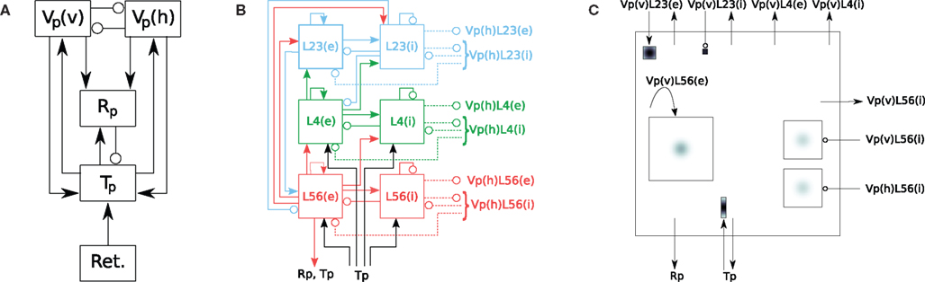
Figure 1. Hierarchy of diagrams of a complex network model (after Hill and Tononi, 2005
). (A) Overview diagram showing only the main parts of the network, i.e., retina (Ret.), thalamus (Tp), thalamic reticular nucleus (Rp), and cortical populations Vp(v) and Vp(h), tuned to vertically and horizontally oriented stimuli, respectively. Arrows mark excitatory, circles inhibitory connections. (B) Detailed diagram of connectivity within cortical population Vp(v). Vp(v) is composed of three cortical layers, each with an excitatory (left) and inhibitory (right) subpopulation. Solid lines represent excitatory, dashed lines inhibitory connections. (C) Detailed rendition of connection masks and kernels projecting onto one cortical subpopulation Vp(v)L56(e) from panel (B), i.e., the excitatory subpopulation of layer 5/6 of Vp(v). Modified from Nordlie et al. (2009
, Figure 6).
A model illustration should present the model accurately and give a precise picture of the implemented model. Illustrations created manually using a computer present the mental image in the mind of the artist, and this might differ from the implemented model. Illustrations created automatically from the same piece of code which generates the network model avoid this disparity. This has two advantages: First, the researcher can use the illustrations to verify the model setup, thus making sure the model is implemented as desired, and second, the illustrations can be used as a starting point for the model description to ensure a correct description of the model.
The aim of an illustration is to convey specific information via the visual channel to the reader. Beck took the complex tube maps and simplified them by removing information to more effectively convey the specific information of greatest interest to the subway users. Travelers interested in the geography had to look elsewhere for that information. The same principles should be applied to illustrations of neuronal network models. A better definition of what to display in illustrations will help both authors and readers of neuronal network model papers to better understand the model.
Tufte (1983
, p. 191) characterizes the designer’s task such:
What is to be sought in designs for the display of information is the clear portrayal of complexity. Not the complication of the simple; rather the task of the designer is to give visual access to the subtle and the difficult – that is, the revelation of the complex.
Faced with a publication practice marked by unsatisfactory illustrations of neuronal network models, we take on the role of the designer (Simon, 1996
) to change this situation for the better by devising new types of network diagrams.
We suggest to split model illustrations into two parts. Box-and-arrow diagrams provide an overview of the network structure. To present details, we propose Connectivity Pattern Tables (CPTs) as a new way of illustrating the existence and properties of connections. CPTs combine and extend elements of connectivity matrices developed by neuroanatomists and -physiologists (Felleman and Essen, 1991
; Scannell et al., 1999
; Dantzker and Callaway, 2000
; Sporns et al., 2000
; Binzegger et al., 2004
; Briggs and Callaway, 2007
; Helmstaedter et al., 2008
; Weiler et al., 2008
) and Hinton diagrams known from artificial neural network research (Hinton et al., 1986
) to the illustration of neuronal network models, for which all design parameters are known explicitly.
Below, we first review principles of visualization, before giving an overview of what needs to be illustrated in a neuronal network model, and how this has been done in the computational neuroscience literature so far. We then present connectivity pattern tables as a new way of illustrating neuronal network connectivity, and describe the ConnPlotter tool for the automatic creation of such illustrations from the network model implementation.
The use of illustrations dates back to cave paintings drawn some 32,000 years ago (Clottes and Féruglio, 2009
), about 25,000 years before the first writing system was developed (Writing, 2008
). In the early days, illustrations were used to communicate ideas, practices and customs. Artists such as Leonardo da Vinci combined illustrations and science, and introduced what is now known as technical drawings (Hulsey, 2002
).
Today, illustrations play an important part in science and are natural elements in scientific publications. The illustrations are technical illustrations rather than technical drawings, differing in their purposes and thus their appearance. Technical drawings are detailed and used for designing and manufacturing artifacts, while technical illustrations are less detailed, with the main purpose of conveying information about an object quickly and clearly (Giemsa, 2007
). When we later refer to illustrations, diagrams or figures, we mean technical illustrations.
A picture is worth more than a thousand words: complex concepts can be described with just a single illustration conveying large amounts of information quickly. This does not make prose redundant, but visual representations aid in transferring knowledge between people, and give insight more efficiently than text (Briscoe, 1996
; APA, 2001
). A good diagram has a clear and deliberate message. It conveys complex ideas in the most simple way without losing precision (Tufte, 1983
; White, 1984
; Briscoe, 1990
; Nicol and Pexman, 2003
).
Visualizing Neuronal Network Connectivity
The description of a neuronal network model in a publication should cover the network architecture, connectivity, and neuron and synapse models. The description is typically in prose, accompanied by a figure (Nordlie et al., 2009
). In the literature we find models ranging from simple models with few parts and connections to larger models with more parts and intricate connectivity. Despite the apparent difference in complexity, we find that all models are visualized in the same manner.
There is seldom more than one figure of the model in a paper on neuronal networks, the sole figure comprising information on network architecture, connectivity, and in some cases also neuron and synapse models. Geometric shapes such as squares, rectangles and circles represent the parts of the network model, while connections are marked by lines linking source and target. A line indicates a connection, and line style or line endings are commonly used to convey information about the connection type, e.g., excitatory or inhibitory, or the connection strength. Typical end-symbols are arrowheads or crossbars. The same symbol may represent different things: crossbars are used to mark excitatory connections in Hayot and Tranchina (2001
, Figure 2) and inhibitory connections in Hill and Tononi (2005
, Figure 1). There is no established common practice in the computational neuroscience literature for how to visualize what, or which notation to use (Nordlie et al., 2009
). In addition, the box-and-arrow diagrams just described do not include connectivity details, e.g., the projection pattern.
For simple network models, the box-and-arrow diagrams fit well, since the number of parts and connections are relatively small. For more complex models, such illustrations are not reasonable, because there is too much information to display. Briscoe (1996
, p. 6) points out that
[t]he most common disaster in illustrating is to include too much information in one figure. Too much information in an illustration confuses and discourages the reader.
To avoid the information overload in a single figure, we suggest to distribute the information between several figures, each showing different hierarchical levels. As an example, we consider the complex thalamocortical model presented by Hill and Tononi (2005)
. Following Nordlie et al. (2009)
, we illustrate this model here using a hierarchy of three drawings in Figure 1
: panel A provides an overall view of the network, panel B details the connectivity within the cortical populations tuned to vertical stimuli, while panel C gives details on projection patterns into a single cortical population.
In spite of the increased clarity provided by hierarchical figures, there is still too much information in, e.g., Figure 1
B. The number of connections are many and line crossings cannot be avoided. This makes it difficult to see which parts connect where, even though sources are given different colors. The seminal network diagram of the primate cortex by Felleman and Essen (1991)
indicates how daunting network illustrations can become.
Connectivity Matrices
Neuronal networks may be described as directed graphs. In graph theory, graphs are commonly described using connectivity matrices. Each row of a connectivity matrix represents the connections (edges) from one graph element (node) to all other nodes. Connectivity matrices are used in several contexts: They are widely used to present connectivity in neuronal networks (see e.g., Felleman and Essen, 1991
; Sporns et al., 2000
; Sporns, 2002
). The CoCoMac-project (http://cocomac.org
) uses connectivity matrices to display the existence of connections in the primate brain. Binzegger et al. (2004)
, Binzegger et al. (2009)
extend connectivity matrices and present in each cell the number of synapses for a connection. The connectivity matrices in Scannell et al. (1999) and Weiler et al. (2008)
show connectivity strength. Dantzker and Callaway (2000) and Briggs and Callaway (2007)
visualize actual input to cortical neurons in the form of connectivity matrices, i.e., input maps, whereas Helmstaedter et al. (2008)
show axonal density maps of cortical layer 4 neurons. Hinton diagrams (Hinton et al., 1986
), a variant of connectivity matrices, are commonly used in the artificial neural network literature to visualize network connectivity. Hinton diagrams show squares or circles with an area proportional to the strength of each connection. Figure 2
A shows a simple network example, and three types of connectivity matrices: panel B displays existence of connections, as in the CoCoMac-matrices, while panel C indicates connection strength by color code, ranging from dark red via yellow to white, as in Binzegger et al. (2004
, 2009
). Finally, panel D displays the same connectivity using a Hinton diagram.

Figure 2. Example network and connectivity matrices. (A) A simple network consisting of four parts a, b, c and d. The intensity I of each connection is marked. Connectivity matrices, based on (B) CoCoMac (http://cocomac.org
), indicating the existence of connections by 0 and 1, (C) Binzegger et al. (2004)
, indicating connection strength by color code ranging from dark red to white, and (D) Hinton-diagrams (Hinton et al., 1986
), indicating connection type and strength by color and area, respectively. In all matrices, sources are represented by rows, targets by columns.
We present here Connectivity Pattern Tables (CPTs) as a compact, machine generatable visualization of connectivity in large neuronal networks, showing not only the existence or strength of a connection, but also its spatial structure. The essential features of CPTs are (i) a clutter-free presentation of connectivity, (ii) high information content with respect to the spatial structure of connectivity, (iii) ability to represent connectivity at several levels of aggregation, and (iv) machine-generation of the visualization from the same script code as used to generate the actual network, with minimal additional user input.
In this section, we introduce the principles of CPTs and illustrate them with three examples. In the next section, we will briefly present our ConnPlotter tool, which automatically generates CPTs from network specifications written using the NEST Topology module (Plesser and Austvoll, 2009
). All CPTs shown here were created using ConnPlotter and are shown without modifications; the same holds for the tables describing the connectivity of the example networks.
Populations, Groups, and Projections
Neuronal network architecture can be described from different perspectives. A cortical network may either be described as a grid of columns, each of which contains neurons in several layers, or as a collection of layers which are grids of neurons. Connectivity in networks, on the other hand, is often described in terms of specific neuron categories, e.g., “thalamic relay cells project to layer 4 pyramidal cells in primary visual cortex.” In our definition of CPTs, we abstract from these details of representation and define connectivity based on three concepts:
Population A two-dimensional sheet of neurons with a given extent in a coordinate system, which may be in physical or stimulus space. Each neuron in a population has a position within the extent. All neurons in a population are treated equally when connections are created. Usually, populations will contain only neurons of one type, but this is not a strict requirement.
Population group A collection of populations. For brevity, we will usually call it just a “group”. Groups are used to structure CPTs and will often represent parts of the brain, such as thalamus or primary visual cortex. Each population must belong to exactly one group.
Projection A rule describing the connectivity between a source and a target population in terms of a convolution as detailed below.
Several simulation tools, such as PyNN and the NEST Topology Module currently support populations and projections as described here (Davison et al., 2008
; Plesser and Austvoll, 2009
).
In the subsequent discussion, we assume for the sake of simplicity that projections are divergent, i.e., that the projection rule describes how to pick target neurons for any given source neuron. Our discussion applies equally for convergent projections (pick source neurons for any target neuron). We will return to the difference between convergent and divergent projections in the discussion.
We require further that some function d(·,·) exists that maps the locations  and
and  of a source and a target neuron onto a displacement vector
  even if source and target populations use different coordinate systems.
and of a source and a target neuron onto a displacement vector even if source and target populations use different coordinate systems.A projection is then defined by the following components:
Source The pre-synaptic (source) population.
Target The post-synaptic (target) population; may be identical to source.
Synapse The type of synapse to use for the connections.
Mask A function  where
where  is the displacement between a source and a target neuron. Connections can only be created if
where is the displacement between a source and a target neuron. Connections can only be created if Kernel A function  of source and target positions. It specifies the probability of creating a connection between source and target neurons with displacement
of source and target positions. It specifies the probability of creating a connection between source and target neurons with displacement Weight The weight w of the connections to be created. This may be a number or a rule for determining the weight, e.g., from a probability distribution.
Delay The delay of the connections, specified in the same way as the weight.
Projections defined in this way imply that the same connection rule applies everywhere between two populations. Mask and kernel could obviously be combined into a single function, but simulators can create connections far more efficiently if the mask is given separately; we therefore consider it a component in its own right.
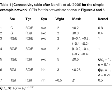
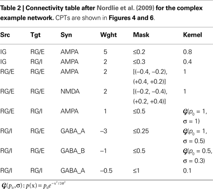
The Simple and Complex Example Network
Tables 1 and 2
show projection information for the two example networks we will use for illustration below. We will refer to the networks as Simple and Complex, respectively. Both networks have two population groups, IG and RG. IG (input group) contains only one anonymous population, while RG (recurrent group) contains populations E and I. Projections in the Simple network use a single synapse type that is interpreted as excitatory for positive weights and as inhibitory for negative weights. The Complex network, in contrast, has AMPA, NMDA, GABAA, and GABAB synapses. All populations in both networks have an extent of 1 × 1 in arbitrary units.
Full Connectivity Pattern Tables
We shall now describe design guidelines for full connectivity pattern tables, i.e., tables showing the detailed connectivity between all populations in a network. For illustration, we show the CPTs for the Simple and Complex examples in Figures 3 and 4
, respectively.
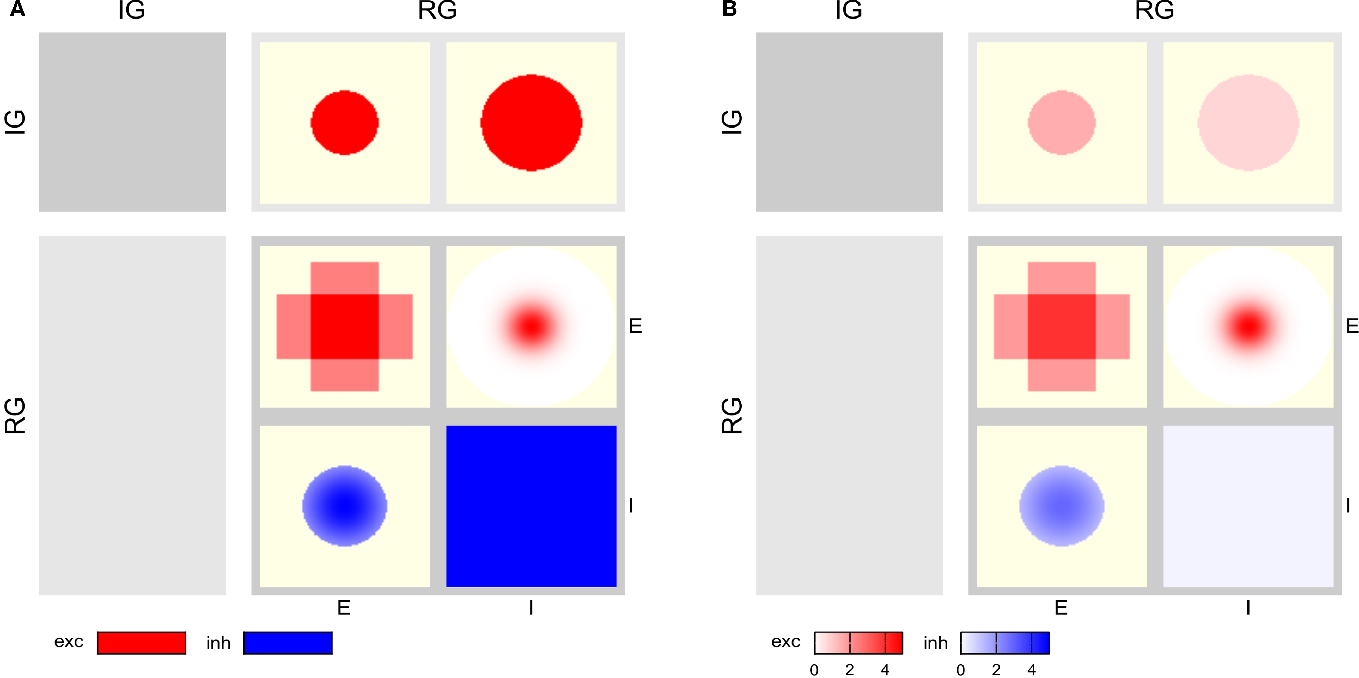
Figure 3. CPTs for the Simple network connectivity defined in Table 1
. Rows represent sources, columns targets. Excitatory connections are shown in red, inhibitory ones in blue. Saturation reflects the connection intensity defined as product of connection probability and synapse weight in arbitrary units. (A) Local color scale for each patch; patches with only a single value show fully saturated color. (B) Global color scale; only the maximum of the Gaussian RG/E→RG/I connection reaches full saturation. This CPT is discussed in detail in the section “Simple network CPT”.
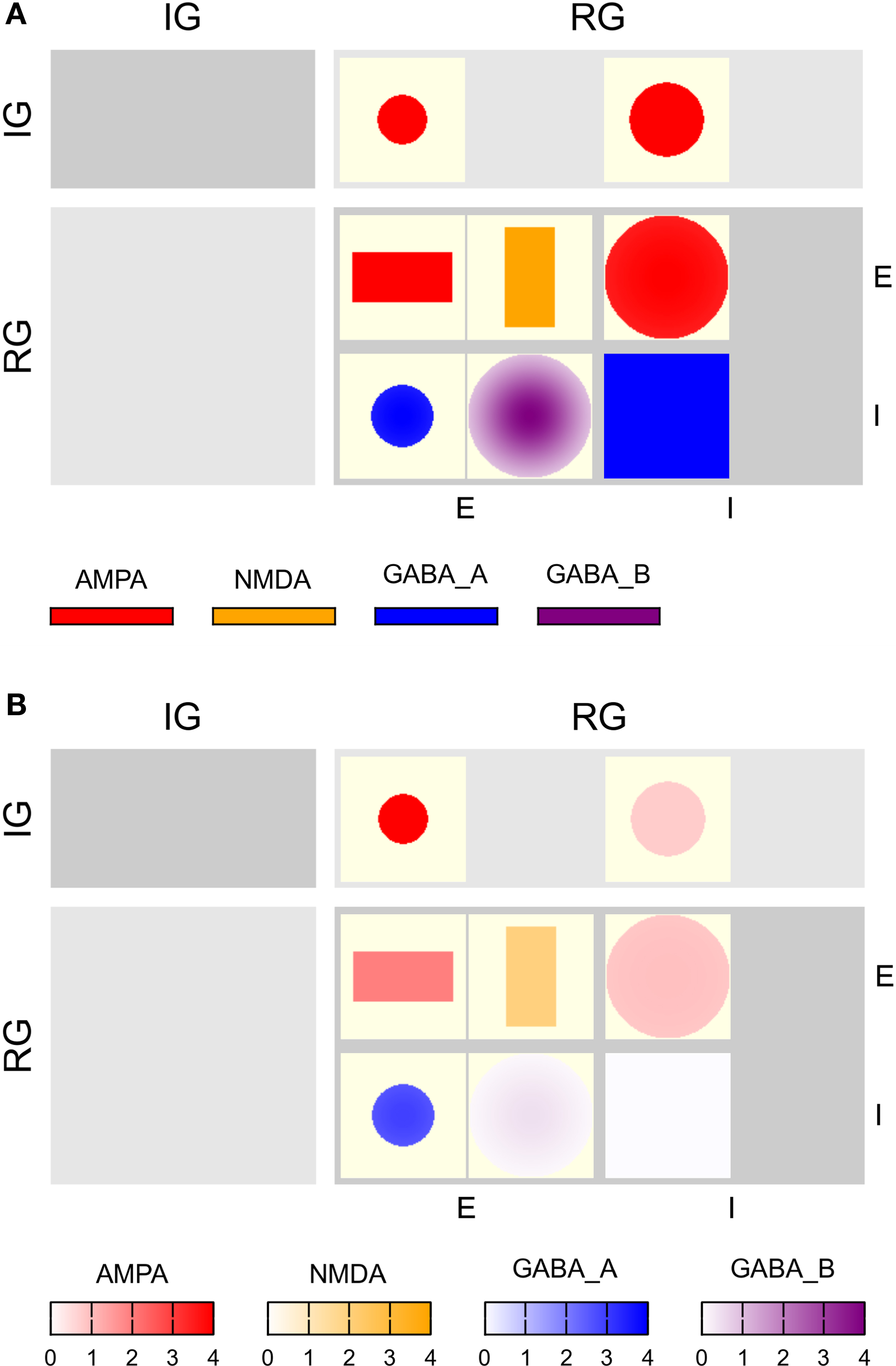
Figure 4. CPT for the Complex network connectivity defined in Table 2
. Full table showing the four different synapse types (AMPA: red, NMDA: orange, GABAA: blue, GABAB: purple) using (A) local and (B) a global color scale. This CPT is discussed in detail in the section “Complex network CPT”.
1. Projections are shown in a table, with one row per source, one column per target population of neurons.
2. Each table entry is a patch, i.e., a rectangle indicating the extent of the target population. It shows the intensity  of the projection from a source neuron to a target neuron displaced by
  . The intensity is defined in the section “Intensity”.
of the projection from a source neuron to a target neuron displaced by . The intensity is defined in the section “Intensity”. 3. Intensities for projections with the same source, target, and synapse type are added.
4. Projections with the same source and target populations, but different synapse type, are shown in neighboring patches.
5. Synapse types are grouped, typically into excitatory (glutamatergic) and inhibitory (gabaergic) synapses: The synapse types of projections between any pair of source and target populations must be from the same group. Grouping is discussed in more detail below.
6. Intensity is indicated by color, from white for I = 0, to fully saturated for maximum intensity. The area of the target population outside the mask is off-white.
7. The color scale of patches across all projections can either be local, i.e., each patch uses its own color scale (Figures 3
A and 4
A), or global, i.e., the same scale is used across all patches in a table (Figures 3
B and 4
B).
8. Colors are assigned to synapse types as follows:
(a) If all projections in a network use the same synapse type, then synapses with positive weight are considered excitatory and shown in red, those with negative weight are considered inhibitory and shown in blue, cf. Figure 3
.
(b) If all projections use a subset of AMPA, NMDA, GABAA, and GABAB synapses, the following colors are used (cf. Figure 4
):
AMPA red;
NMDA orange;
GABAA blue;
GABAB purple.
(c) In all other cases, the user needs to define colors herself.
9. Population groups are indicated by gray background rectangles; a darker shade of gray is used to emphasize the diagonal.
10. Labels for population groups are shown in the left and top margins, labels for populations in the right and bottom margins.
11. Projections excluding autapses (connections from a neuron onto itself) are marked by a crossed-out “A” in the upper right corner of the patch, projections excluding multapses (multiple connections between one pair of neurons) with a crossed-out “M”.
The grouping of synapse types reflects Dale’s law (Shepherd, 1998
), which stipulates that neurons only secrete one type of neurotransmitter, so that one will have a combination of either AMPA and NMDA or GABAA and GABAB projections, but not of, e.g., AMPA and GABAA. An example is shown in Figure 4
. By default, AMPA and NMDA form one group, GABAA and GABAB a second group. This grouping can be freely defined by the user, though, so that networks violating Dale’s law can also be presented by CPTs.
Local color scales bring forth the structure in individual projections, but give no impression of the relative strength of projections. A global color scale, on the other hand, is useful to judge the relative strength of different projections in a network. To avoid that a single strong connection “drowns” detail among weaker connections (cf. Figures 3
B and 4
B), the user can choose the limits of the global color scale; see Figure 5
C for an example.
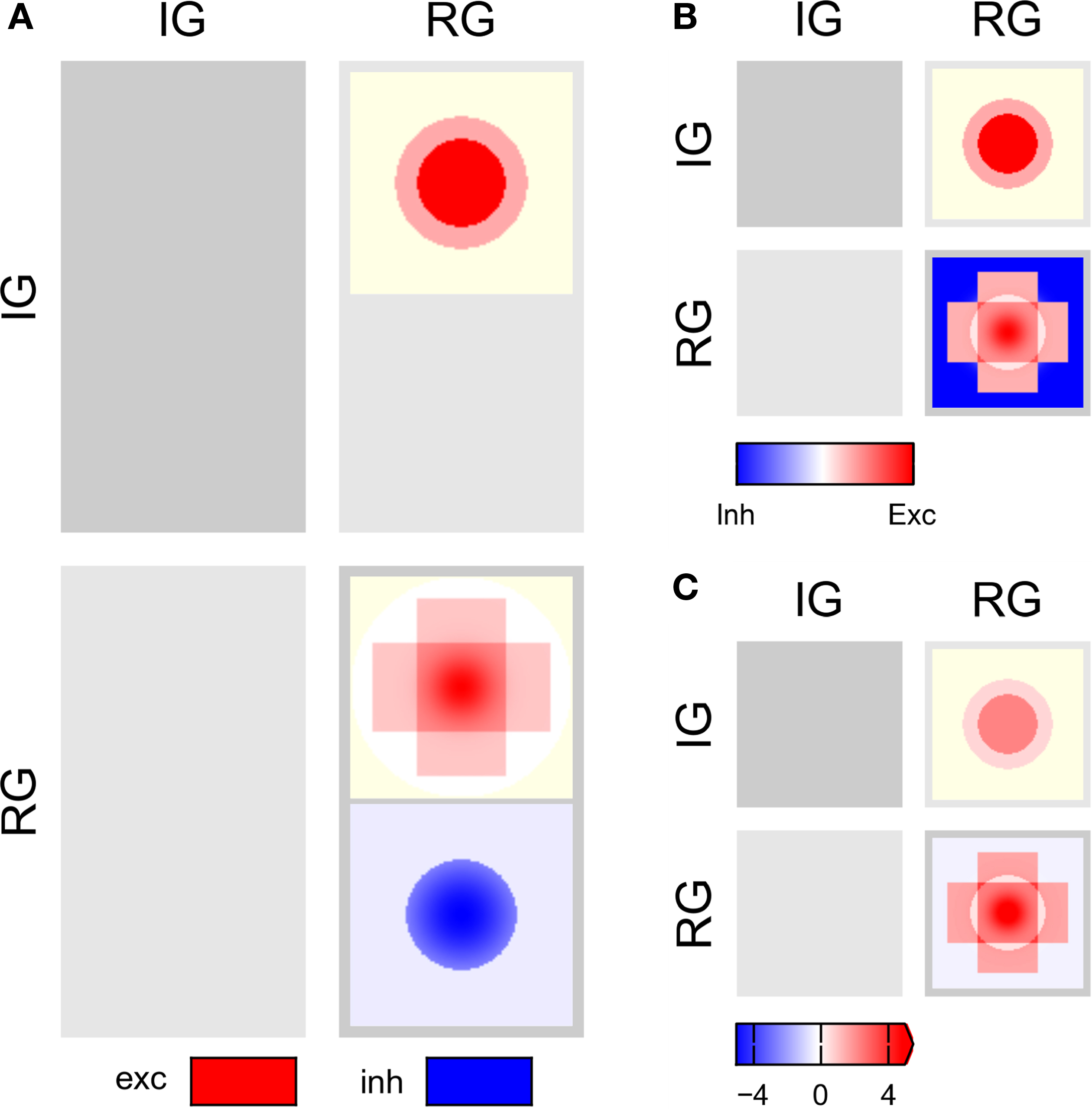
Figure 5. Aggregated CPTs for the Simple network. (A) Connections for each source/target pair of population groups are aggregated, but synapse types kept separate. (B) Connections aggregated across layers and synapse types. As for all CPTs aggregating across synapse types, the color scale ranges from blue (most inhibitory) via white (neutral) to most excitatory (red). (C) As in panel (B), but now using a global scale for colors in all patches. The arrow at the right end of the color bar indicates that the CPT contains values >5.
When using a global color scale, proper color bars are displayed at the bottom of the CPT. If the user has defined the limits of the color scale manually and some intensity values are outside these limits, this is indicated by an arrowhead at the respective end of the color bar, as illustrated in Figure 5
C. Individual color bars for each patch in a CPT with local color scales would lead to significant visual clutter. In this case, therefore, a plain legend is shown, mapping synapse types to colors.
Intensity
It is not a priori clear what measure one should use to indicate the strength of a projection. We have chosen to define the intensity of a projection as follows: The intensity  is the product of the probability of a connection being created, and the weight of the connection,
 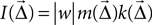 . If the weight is given as a distribution, the mean is used. This choice is motivated by Binzegger et al. (2004)
, who chose line width in this manner. As an alternative, one may also consider the probability of connection alone, given by
. If the weight is given as a distribution, the mean is used. This choice is motivated by Binzegger et al. (2004)
, who chose line width in this manner. As an alternative, one may also consider the probability of connection alone, given by  , as the intensity.
is the product of the probability of a connection being created, and the weight of the connection, . If the weight is given as a distribution, the mean is used. This choice is motivated by Binzegger et al. (2004)
, who chose line width in this manner. As an alternative, one may also consider the probability of connection alone, given by , as the intensity.The actual effect of incoming spikes on the membrane potential may depend significantly on the state of the neuron. Input through inhibitory synapses, e.g., will have larger effects when the neuron is depolarized and thus further from the synaptic reversal potential, and NMDA synapses will be ineffective unless the neuron is sufficiently depolarized. To capture this in a – if simplistic – fashion, we propose a third alternative definition of the intensity in terms of an estimate of the total charge moved across the membrane in response to one incoming spike. Let

be the synaptic current, where w is the synaptic weight, g(t) describes the time course of the synaptic conductance in response to a single input spike as a function of time alone, m(V) a function describing a voltage dependence of the synapse, while Erev is the reversal potential. m(V) will be unity for most synapse types except NMDA. The total charge deposited (tcd) due to a single input spike at t = 0 is then

We now assume that a single input spike evokes only small changes in membrane potential, so that we may fix V = V0 when computing Q. We thus approximate the total charge deposited as

and finally define the intensity as product of charge deposited and probability of connection:

Note that the synaptic weight w is included in Qtcd. Examples of CPTs based on Itcd will be given in the section “CPT for a simplified Hill-Tononi network”.
Aggregated Connectivity Pattern Tables
CPTs as described above represent each projection individually. CPTs for large networks may be quite large. Structuring the CPTs by population groups provides some overview, but in many cases it will be of interest to condense information. To this end, we define several types of aggregated CPTs:
By group For each synapse type, intensities for all population pairs in a pair of source and target populations groups are summed (cf. Figures 5
A and 6
A).
By synapse For each pair of source and target populations, intensities are summed across synapse types (cf. Figure 6
B).
By group and synapse As aggregation by group, but summed across synapse types, too (cf. Figures 5
B and 6
C).
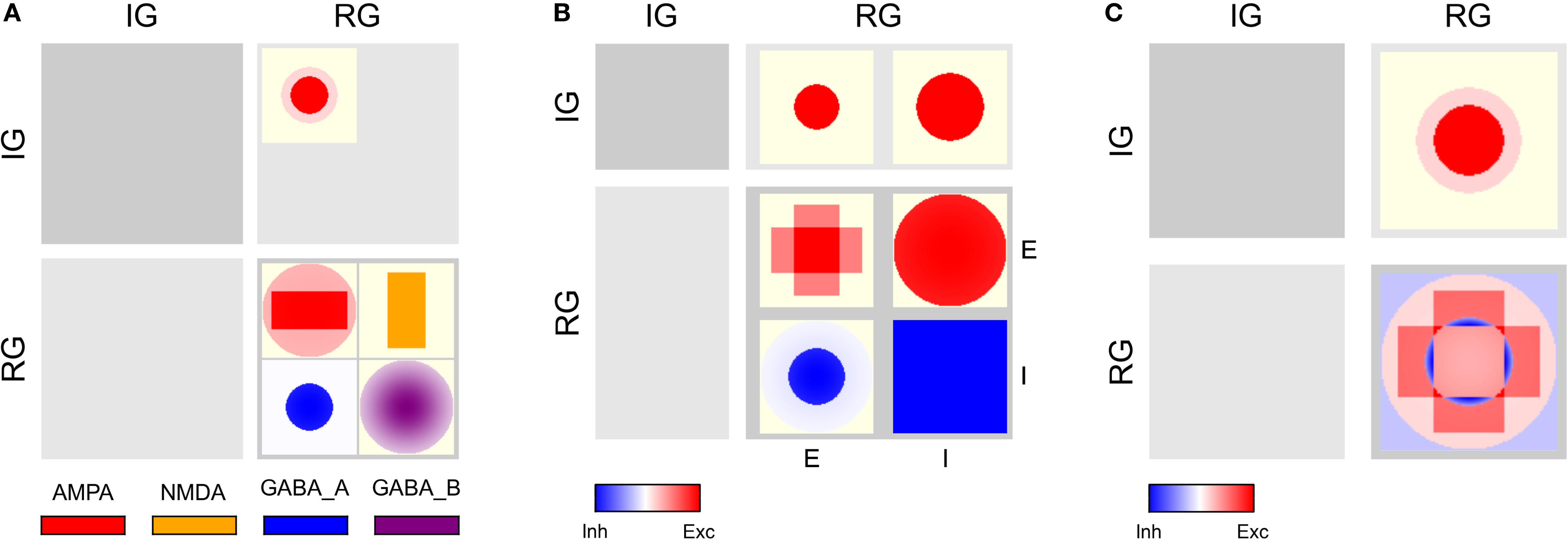
Figure 6. Aggregated CPTs for the Complex network show in Figure 4
. (A) Connectivity aggregated across groups, but not synapse types. (B) Connectivity aggregated across synapse types for each source/target pair of populations, i.e., combining either AMPA and NMDA or GABAA and GABAB. (C) Connectivity aggregated across groups and synapse types.
Aggregated CPTs are displayed in the same way as full CPTs, with the following additions:
12. When summing across synapse types, intensity  is first computed for each synapse type individually. Intensities are then weighted with +1 for excitatory (AMPA, NMDA) and −1 for inhibitory (GABAA, GABAB) synapse types. Different weights may be used.
is first computed for each synapse type individually. Intensities are then weighted with +1 for excitatory (AMPA, NMDA) and −1 for inhibitory (GABAA, GABAB) synapse types. Different weights may be used.13. The resulting intensity is shown on a blue-white-red color scale as follows:
(a) I < 0 is shown in blue with saturation ∼|I|.
(b) I = 0 is shown in white.
(c) I > 0 is shown in red with saturation ∼I.
(d) When using local color scales, the red and blue parts of the scale are scaled independently: fully saturated red may correspond to I = 10, while fully saturated blue corresponds to I = −0.5 (cf. Figure 5
B).
(e) When using a global color scale, red and blue scales are coupled by default, i.e., lower and upper limits of the color scale have the same absolute value (cf. Figure 5
C). The user can set different limits.
14. When grouping by population groups, no population labels are shown.
CPT: Examples
We shall now briefly review the Simple and Complex example networks to elucidate some properties of connectivity pattern tables, before we turn to a large network model taken from the literature.
Simple network CPT
The full CPT for the Simple network is shown in Figure 3
with local and global color scales. The left column is empty, as the IG population group receives no input. The patches in the right column show the projections onto the RG population group. This column is split in two sub-columns, marked E and I at the bottom, each representing projections onto one of the populations in the RG group.
The top row shows projections onto the RG group from the IG group: the left patch represents the projection onto the E population, the right onto the I population, corresponding to rows 1–2 in Table 1
, respectively. Both projections are excitatory and have constant intensity within a circular mask.
The bottom row of the CPT shows projections from the RG group onto itself. It is split into two sub-rows, representing projections from E and I populations, respectively. The E→E projection is the sum of the two rectangular projections defined by rows 3–4 in Table 1
, as stipulated by design guideline 3. The E→I projection has a narrow Gaussian intensity profile in a mask filling almost the entire extent of the population (row 5), while the I→E projection has a wider Gaussian profile inside a narrower mask (row 6). The I→I projection has constant intensity filling the full extent of the population (row 7). Projections emanating from the E population are excitatory (red), those from the I population inhibitory (blue).
Figure 3
B shows the same CPT with a global color scale. This reveals that the projection from the IG group to the RG/E population is stronger than to the RG/I population, and that the highest intensity is at the center of the RG/E→I projection. The RG/I→I projection is very weak, but does not vanish: if the latter were the case, the patch would be off-white, not light blue.
Figure 5
A shows the CPT for the Simple network aggregated by population groups: Projections to and from populations E and I in the RG group are now combined. The IG→RG projection is purely excitatory, whence we have only a single patch with two superimposed circles. Inside the RG layer, we have excitatory as well as inhibitory projections, and thus two patches. The upper (red) patch combines projections from the E population to the E and I populations – note the Gaussian at the center of the cross. The lower (blue) patch combines the Gaussian and flat projections from the I population to the E and I populations. The flat part is shown as a very light shade of blue only, as it is much weaker than the Gaussian center. Note that the two patches are not combined, as they represent two different synapse types, excitatory and inhibitory.
In Figure 5
B projections are combined by group and synapse type resulting in a 2 × 2 matrix of patches. The IG→RG projection is purely excitatory and thus shows the red part of the color scale only. The aggregated recurrent projection, in contrast, combines excitatory and inhibitory projections and thus extends to the blue part of the color scale, too. The flat inhibitory surround is shown in saturated blue even though it is very weak, because the red and blue color scales are decoupled. Figure 5
C shows the same aggregated CPT, but with a global scale limited to [−5, +5]. Now the weakness of the inhibitory surround becomes apparent.
Complex network CPT
The full CPTs for the Complex network shown in Figure 4
differ from the Simple network as follows: For each source/target pair, there is space for two patches side-by-side, although synapses of both applicable types occur only for the projections from RG/E (AMPA, NMDA) and RG/I (GABAA, GABAB) to RG/E. Figure 6
A shows projections combined by source/target pairs: For each pair, we have a square of four patches, with the excitatory synapse types on top, inhibitory below. Aggregating across synapse types for each source/target population pair gives the aggregated CPT in Figure 6
B, while Figure 6
C shows the aggregation across synapses and populations.
CPT for a simplified Hill-Tononi network
To demonstrate the applicability of connectivity pattern tables to “real life” network models, we present connectivity pattern tables of a simplified version of a large thalamocortical model investigated by Hill and Tononi (2005)
. This model comprises five population groups: retina (Ret), thalamus (Tp), reticular nucleus (Rp), and horizontally and vertically tuned primary visual cortex (Vp_h, Vp_v); we left out the secondary pathway with groups Ts, Rs, Vs_h, Vs_c, and Vs_v. The populations in each population group are summarized in Table 3
. Each population spans an extent of 8° × 8° of visual angle. Figure 1
illustrates the model: Panel A shows the overall architecture between population groups, while panel B presents the detailed connectivity between populations in group Vp_v. The large number of connections makes this figure difficult to read, and it does not provide any information about the spatial profile of the projections. Figure 1
C was a first attempt to include these spatial profiles, but contains only projections onto one population (Nordlie et al., 2009
). The figures in all three panels were created manually.
The full CPT for this model, shown in Figure 7
, provides complete connectivity information. Reading from top to bottom, we find focused retinal input to relay cells and interneurons in the thalamus. Interneurons in thalamus inhibit themselves, while relay cells make oriented and non-oriented projections to the cortical areas, as well as axon collaterals to Rp. Rp in turn inhibits both populations in Tp via GABAA and GABAB synapses, while self-inhibiting via GABAB only. Further down in the Tp and Rp columns, we note the corticothalamic feedback from layer 5/6 pyramidal cells to Tp and Rp. Towards the bottom right of the CPT, we find a matrix of 2 × 2 blocks representing intracortical connectivity. The two blocks on the main diagonal show connectivity within the Vp_h and Vp_v groups, respectively, while the off-diagonal blocks show the projections from Vp_h onto Vp_v and vice versa. The latter projections are exclusively inhibitory. One also sees easily that excitatory connections within a single layer generally are much wider than from one layer to another, and that GABAB projections are much more focused than GABAA projections.
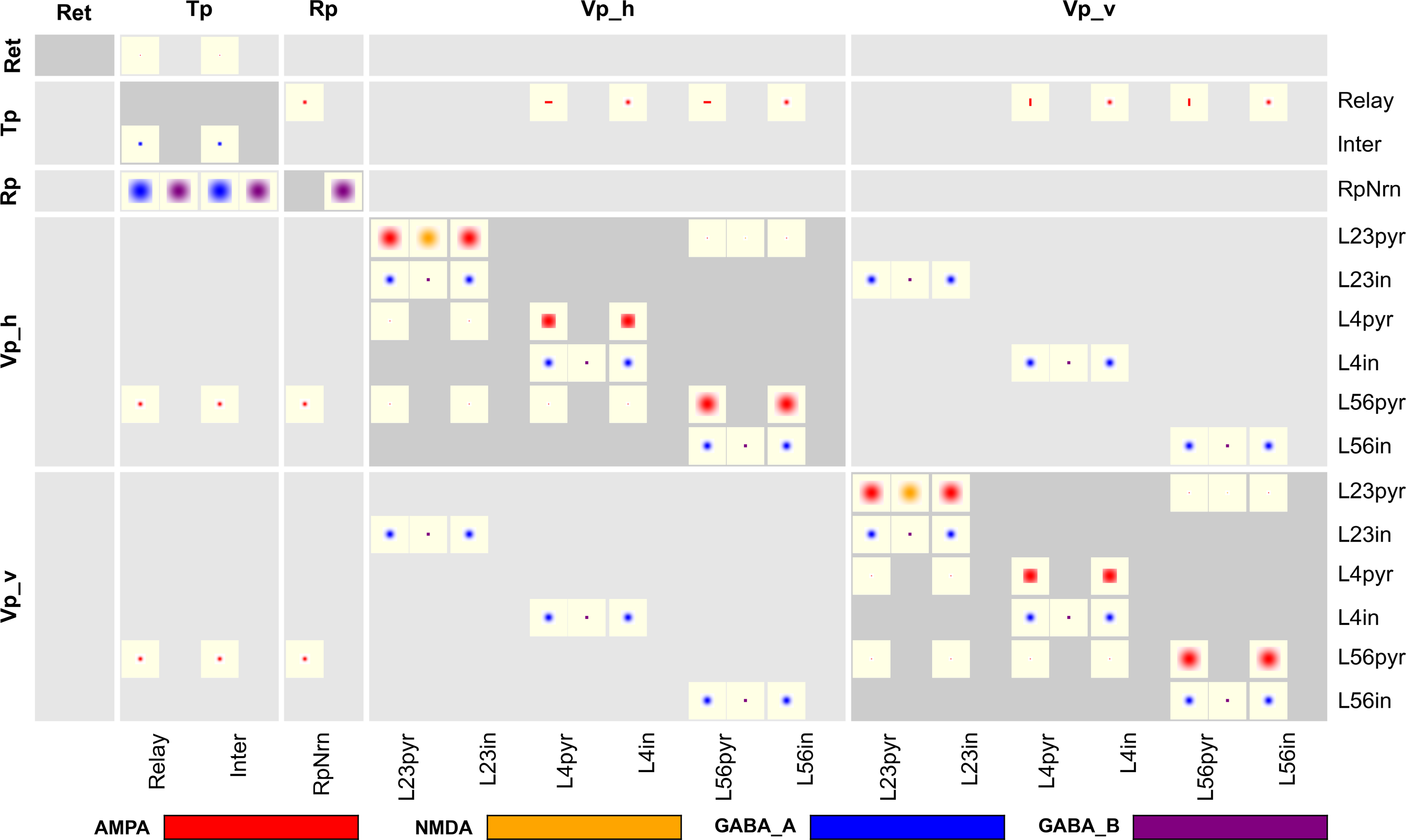
Figure 7. Full CPT for the Hill-Tononi model reduced to the primary pathway (Hill and Tononi, 2005
). Layers are retina (Ret), thalamus (Tp; two populations: relay cells and interneurons), reticular nucleus (Rp), and horizontal and vertically tuned primary visual cortex (Vp_h, Vp_v); the latter two layers have six populations each, representing pyramidal cells and interneurons in layers 2/3, 4, and 5/6. Synapse types are AMPA, NMDA, GABAA, and GABAB, with the same color code as in Figure 4
. Note the rectangular projections from population Tp/Relay to Vp_h and Vp_v.
Figure 8
presents aggregated CPTs for our version of the Hill-Tononi model. In panel A, projections are summed across synapses and in panel B across populations, while panels C and D show CPTs aggregated across synapses and populations using local and global color scales, respectively. The latter CPTs bring out the overall connectivity in the network comparable to Figure 1
A, but contain much more information.
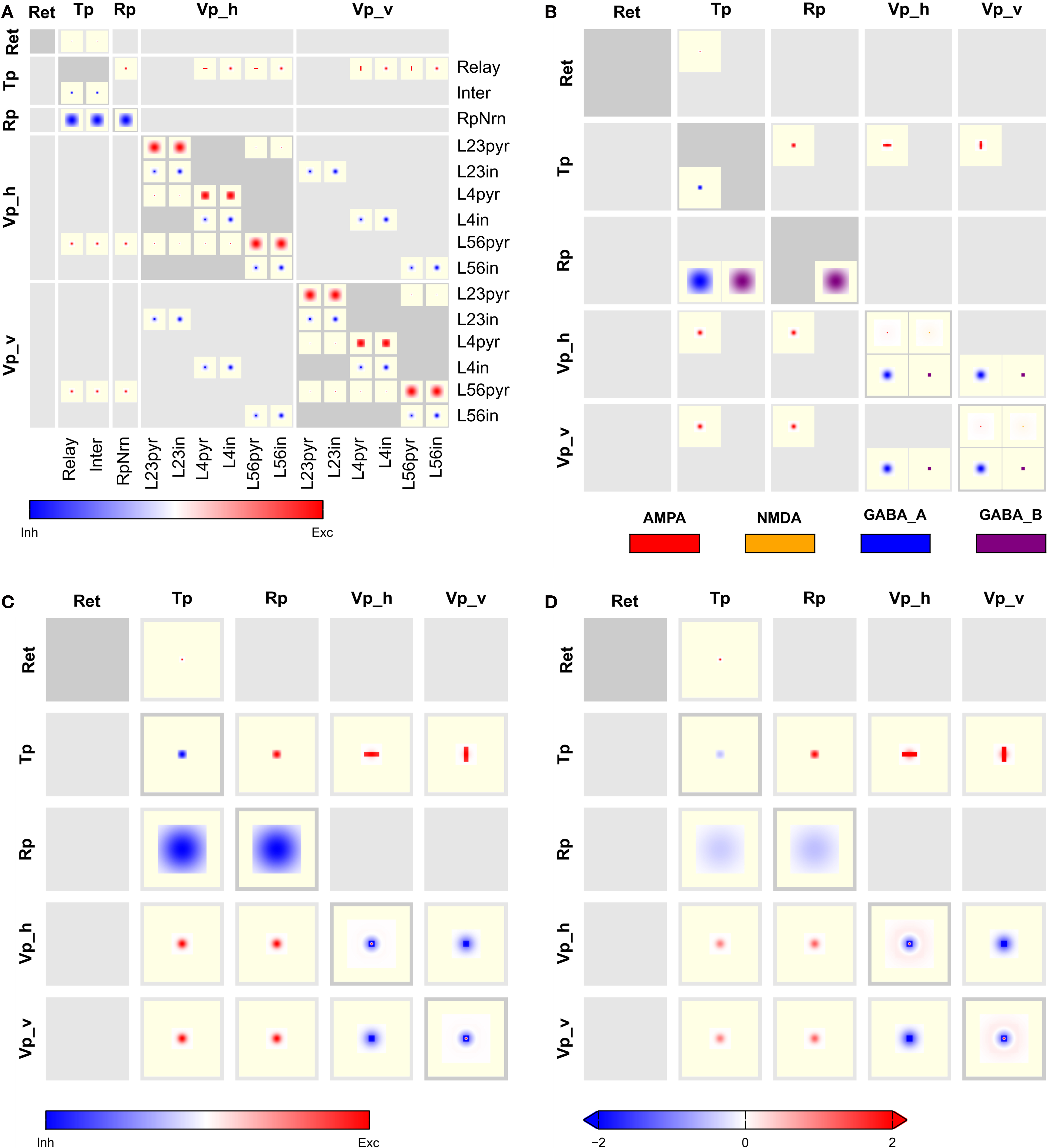
Figure 8. Aggregated CPTs for the Hill-Tononi model from Figure 7
. (A) Connectivity aggregated across synapse types for each population pair. (B) Connectivity combined across populations in each group, but not across synapse types. (C) As in panel (B), but also aggregated across synapse types. (D) As in panel (C), but with a global color scale limited to [−2,2].
Figure 9
, finally, illustrates how CPTs may be used to reveal differences in effective connectivity as networks are in different operating regimes. In this figure, we show intensity Itcd defined in terms of total charge deposited according to Eq. 4. Figure 9
A shows connectivity for a network in which all populations are in a “down” state (Vm = –70 mV), while Figure 9
B shows connectivity in the same network in an “up” state (Vm = –50 mV). A comparison of the CPTs reveals significantly stronger inhibition within cortex at intermediate distances in the “up” state. CPTs may thus give new insights into network properties under different circumstances.
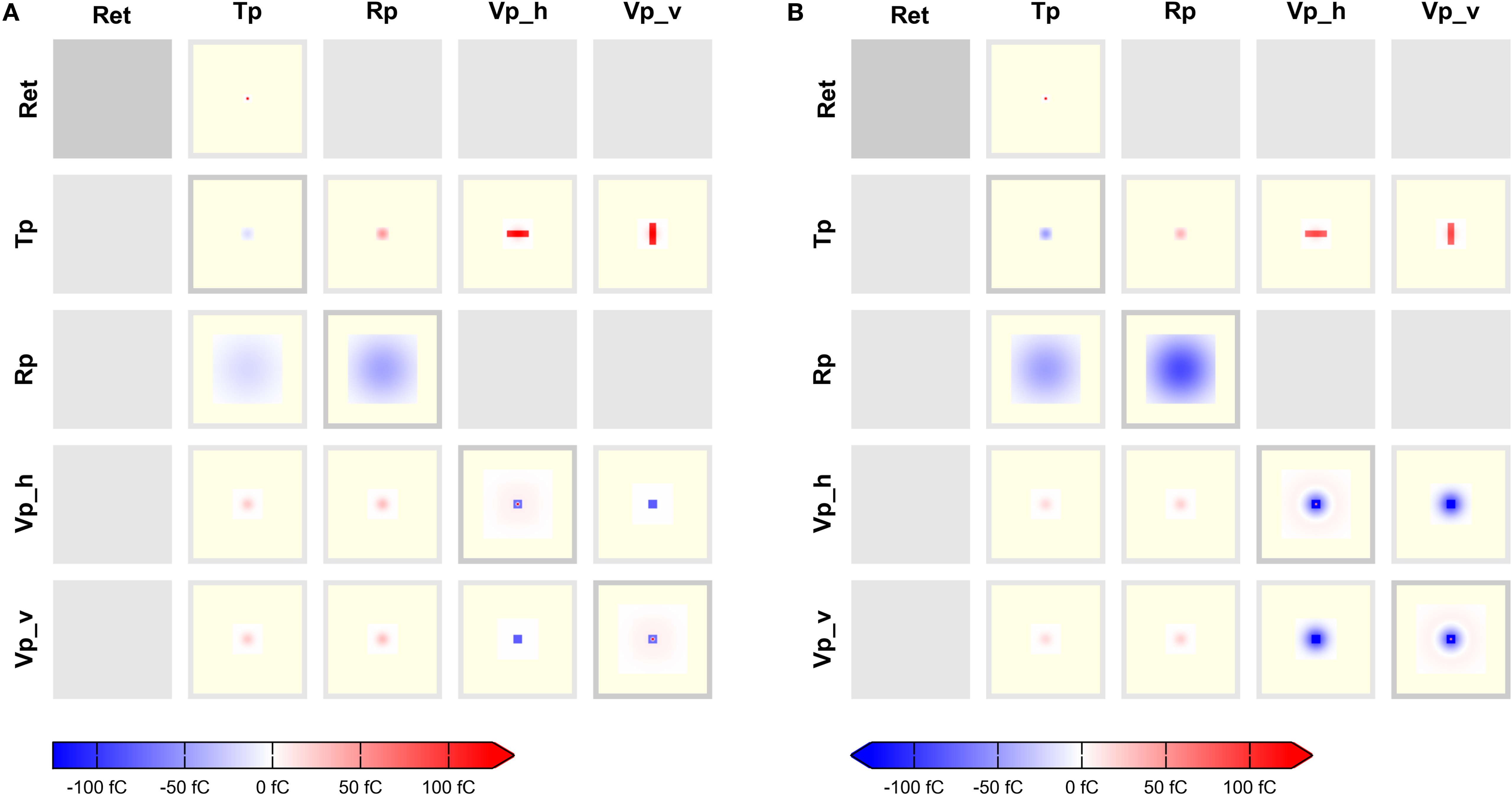
Figure 9. Aggregated CPTs based on total charge deposited. The CPTs shown here are equivalent to Figure 8
D, but intensity is now Itcd defined in terms of total charge deposited in femtocoulomb, cf. Eq. 4 for membrane potential (A) Vm = –70 mV and (B) Vm = –50 mV, respectively. The color scale is the same for both figures. Note the difference in mid-range inhibition in intracortical connections.
We have created the ConnPlotter, a Python package, to allow scientists to generate connectivity pattern tables easily. Our most important aim was to facilitate automatic generation of CPTs directly from the same script code used to create the model for simulation. At present, the ConnPlotter tool can visualize network definitions written for the NEST Topology module (Plesser and Austvoll, 2009
). The ConnPlotter package is available as supplementary material to this paper under an open source license.
In this section, we shall briefly present the ConnPlotter tool and show how networks can be specified in a way that allows visualization with ConnPlotter and simulation using the NEST Topology module. A comprehensive tutorial for ConnPlotter is included as Supplementary Material to this paper. First we shall introduce some NEST Topology concepts.
Nest Topology Concepts
Neuronal networks can be described from different perspectives, as discussed in the section “Populations, groups, and projections”. Connectivity pattern tables present a network as one or several groups of populations. Each population has an extent, but aside from their location, all neurons in a population are considered equal when creating connections.
The Topology module, in contrast, describes a network as one or several two-dimensional layers, each with a spatial extent. Each layer element has a location within the layer, and may consist of one or more neurons of the same or different types. The Simple network introduced in the section “The simple and complex example network” would be constructed in the Topology module as two layers, IG and RG. Each element of layer IG is a single Poisson generator, while each element of layer RG consists of an E and an I neuron. Connections are specified by giving the source and target layers, as well as the source and target neuron types for a projection. If no source or target neuron type is given, all neurons in each element are treated equally.
ConnPlotter matches the Topology module view of the network to the connectivity pattern view as follows:
• Layers are treated as population groups.
• Populations are inferred from the source and target layer and neuron specifications: If any projection in a network has source (or target) layer RG and neuron E, then RG/E is inferred as a population.
• Layers with single-neuron elements are treated as population groups with a single population, which may be anonymous.
• The extent of a population is identical to the extent of the layer to which it belongs.
Thus, the Simple network has layers IG and RG, corresponding to population groups IG and RG. Group IG has a single anonymous population, RG has the populations E and I.
Specifying Networks
We will use the Simple network to illustrate how to specify networks for NEST Topology and ConnPlotter. For details on NEST Topology network specifications, see Austvoll (2009)
. Networks are specified by three lists: the model list (see “Simulating networks”), the layer list and the connection list.
The layer list defines all layers in the network, especially size, extent and elements. For the Simple network, the layer list is
The tuples in the list contain the layer name first, followed by a dictionary specifying layer properties, in this case a 40 × 40 grid of elements spanning an area of 1 × 1 in arbitrary units.
The connection list specifies all projections in the network. We show only two entries of the Simple network connection list here for brevity:
Each entry is a tuple containing source layer, target layer, and a dictionary specifying projection details. The combination of a layer with the neuron type specified for sources or targets in the dictionary defines a population in the sense of connectivity patterns, as discussed in the section “NEST topology concepts”. In the last tuple in the code snippet above,
RG appears both as source and target layer. The sources and targets entry in the dictionary indicate that the projection is from neuron of type E to neurons of type I, thus defining populations RG/E and RG/I. The connection_type entry instructs the NEST Topology module to select neurons targets for each source neuron.Visualizing Networks
A network is visualized as a connectivity pattern table by creating a
ConnectionPattern object and then calling its plot method: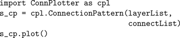
This yields the full CPT shown in Figure 3
A. Population groups (layers) are ordered in the CPT as in the layer list, while populations are ordered alphabetically from left to right and top to bottom.
The remaining CPTs of the Simple model were drawn with subsequent calls of the
plot() methods with different arguments:Figure 3
B Full CPT with global color scale:

Figure 5
A Aggregated by population group (i.e., by layer), local color scales:

Figure 5
B Aggregated by group and synapse type, local color scales:

Figure 5
C Aggregated by group and synapse type, global color scale limited to [−5,5]:

Each of these method invocations will open a new figure window. CPTs are written directly to a file if one is given; in this case, one may also specify the total width of the CPT figure in millimeters:

The appearance of CPTs, e.g., font properties and background colors, can be adjusted to a considerable degree. ConnPlotter can be configured freely to handle networks with other synapse types than plain excitatory and inhibitory (same
synapse_model for all projections, positive and negative weights) or AMPA, NMDA, GABAA, and GABAB. Please see the Tutorial included as Supplementary Material and the online help for details.Simulating Networks
To simulate a network using NEST, we need to complement the layer and connection lists with a model list that maps native NEST neuron models to the models used in the network. For the Simple network, we have
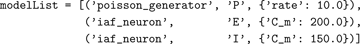
Each list element is a tuple containing the name of the native NEST model, the model name used in the network, and a dictionary providing parameters for the model.
Once these three lists are defined, we can simulate the network in NEST using the PyNEST interface (Eppler et al., 2008
) by iterating over the lists to create models, layers and connections. The only challenge is that we need to turn the layer names given in the layer list into Python variable names. We achieve this by use of the
exec statement. Any network can then be created using the following code: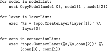
We have proposed here connectivity pattern tables as a new approach to visualizing neuronal network connectivity. CPTs are a natural extension to complex neuronal network models of similar visualization techniques used in neuroanatomy and -physiology (Felleman and Essen, 1991
; Scannell et al., 1999
; Dantzker and Callaway, 2000
; Sporns et al., 2000
; Briggs and Callaway, 2007
; Helmstaedter et al., 2008
; Weiler et al., 2008
), and artificial neural network research (Hinton et al., 1986
). They are complementary to the box-and-arrow network diagrams commonly found in the computational neuroscience literature (Nordlie et al., 2009
). We believe that CPTs have considerable advantages compared to existing styles of network visualization:
1. CPTs provide significantly more information, as the full spatial structure and relative strength of projections are revealed, not only their existence. The aggregated CPTs of the Hill-Tononi model in Figures 8
C,D provide much more detail about the connectivity in the model than the corresponding box-and-arrow diagram in Figure 1
A.
2. CPTs showing intensity defined in terms of total charge deposited reveal differences in effective connectivity in different networks states, as illustrated in Figure 9
. This information is not available otherwise.
3. CPTs are clutter-free by construction: there are no lines connecting boxes and thus no confusing line crossings. Compare, e.g., the full CPT for the Hill-Tononi model in Figure 7
with the box-and-arrow diagram in Figure 1
B, which represents only the connectivity within population group Vp_v.
4. CPTs can be created automatically from the same network specification used to generate the actual network for simulation. This allows scientists to routinely explore their network architectures visually while working with them, as well as to easily create up-to-date figures for publication.
5. CPTs at different levels of detail can be created automatically, allowing inspection or presentation of different aspects of network connectivity.
This should make CPTs a useful tool in the hand of computational neuroscientists, facilitating the interactive development of models, the detection of errors in model specifications, and the effective communication of network connectivities in presentations and publications. In practice, we observed that CPTs with local color scales are most useful in “debugging” network definition scripts, as it is easy to detect missing or extraneous connections, or connections patterns of wrong shape or synapse type. For presentation purposes, and especially for the comparison of CPTs showing state-dependent connectivity based on the total charge deposited, a global color scale with suitably chosen limits appears most valuable.
Our ConnPlotter package demonstrates that CPTs can indeed be created automatically, as stated above, and should allow scientists to generate CPTs for their models with reasonable ease. This said, we would like to remark that we consider ConnPlotter to be usable and reasonably stable, but by no means a complete tool for generating CPTs. Further development of the tool will depend on the reception of the connectivity pattern tables in the community.
A number of open issues and limitations remain. Most of these relate to the scientific interpretation of connectivity, rather than to technical aspects. We consider the following issues particularly relevant.
Intensity We propose three alternative definitions of the intensity of a projection: probability only, probability times weight (default) and probability times total charge deposited; in the latter case, the intensity also depends on the membrane potential in the target population. The first two definitions reflect mostly the static architecture of the network, the latter may be used to illustrate the effective connectivity in a network in different states, such as “up” and “down” states in cortex.
If different populations have different densities of neurons, considering just probability, weight, or total charge deposited when defining the intensity of a projection may give misleading impressions of the relative impact of different projections. In such cases, it may be useful to include the source and/or target population density in the definition of intensity.
Divergence/Convergence We have assumed so far that all projections are divergent, i.e., that connection targets are chosen according to mask and kernel for each neuron in the source population. Models describing connections as convergent can be handled in two ways: (i) CPTs are created as before, but each patch is interpreted as showing how to select source neurons, not target neurons. (ii) The convolutions described by mask and kernel are inverted, so that the convergent description becomes a divergent one. CPTs are then drawn using the divergent mask and kernel.
The latter approach has two advantages. First, it can be used in cases where some projections are described as divergent, some as convergent, as in the original model by Hill and Tononi (2005)
. That model describes all projections as divergent, except for the rectangular thalamocortical projections. In our implementation, we inverted these projections to divergent projections. The second advantage is that CPTs defining intensity in terms of total current deposited can be drawn only for divergent projections, since the membrane potential of the target population determines the effective strength of synaptic input.
Patchy projections Some cortical neurons show patchy connection patterns (Douglas and Martin, 2004
): connections are clustered in space. To represent such patchy projections fully, one would have to visualize the distribution of the patch centers as well as the distribution of connections around these centers. It is not a priori clear how to integrate both types of information into a single figure.
Subcortical networks CPTs are tailored to layered networks as are typical for cortex and parts of the thalamus. Applying CPTs to other types of networks, e.g., models of the basal ganglia, may require modified designs.
Dependent kernels CPTs visualize projections defined by convolutions, cf. section “Populations, groups, and projections”, which implies that the same mask and kernel applies everywhere between two populations. Projection rules which depend not only on the displacement between, but also on the actual location of source and target neurons, e.g., their retinal eccentricities, cannot be presented fully using CPTs. One might, though, draw separate CPTs illustrating kernels for various eccentricities.
Some authors, notably Troyer et al. (1998)
, have presented models in which the projections from population B to population C depend on the correlations between connections from population A to population B. Thus, the effective kernel for the B→C projection is a convolution of the A→B kernel with a nominal B→C kernel. CPTs for such dependent kernels are outside the scope of the design guidelines given here.
Aggregation by synapse When projections are aggregated by synapse, intensities for different synapse types are simply weighted with a scalar factor, by default +1 for excitatory and −1 for inhibitory synapses. It is by no means clear that this will give the best rendition of the combined effect of the projections, in particular for non-linear synapses.
Coordinate systems We have assumed here that all layers use the same 2D coordinate system, so that distances between source and target neurons can be calculated easily. This assumption can be relaxed, as long as a transformation is provided that maps locations between source and target layers. Similarly, one could employ mixed coordinate systems, in which, e.g., one axis represents location in the visual field and the other stimulus orientation. Masks and kernels would then have to be defined in terms of this coordinate system.
As real brains are three-dimensional structures, it would be advantageous to be able to visualize connectivity in three dimensions. We believe that this would be possible in a meaningful way only as part of an interactive tool.
Connectivity for one-dimensional networks could, on the other hand, easily be displayed using CPTs. In this case, one would show in each patch the pertaining intensity as a one-dimensional function plot.
Boundary conditions Our design guidelines, and the current implementation of ConnPlotter, silently assume that projection kernels are cut-off at the edge of a populations extent.
Delay Connection delays are entirely ignored in CPTs: we simply lack the third dimension to represent time. One option would be to visualize the distribution of delays by drawing CPTs in which the delay defines the intensity.
Simulator support At present, ConnPlotter is tied closely to the NEST Topology module. The basic concepts of the Topology module are quite general, though, and match the “Populations” and “Projections” of the PyNN simulator wrapper quite well (Davison et al., 2008
). ConnPlotter should thus be easily adaptable to, e.g., PyNN. CPTs using intensity defined in terms of total charge deposited (cf. Eq. 4) require that the simulator provides access to the value of  either directly or indirectly.
either directly or indirectly.We found in the work with connectivity pattern tables and the ConnPlotter tool that the field lacks a sufficiently established nomenclature for components of neuronal networks. In particular, construction and connection of networks are often described from quite different perspectives, as discussed in the sections “Populations, groups, and projections” and “NEST topology concepts”. While the construction perspective to a large degree builds on terminology from neuroanatomy (e.g., cortical layers and columns), the connection view of networks seems to have received little attention in the past (Austvoll, 2007
), whence there is no established terminology. We are optimistic that the increasing attention to model exchange and systematic model description (Cannon et al., 2007
; Gleeson et al., 2008
; Nordlie et al., 2009
), and in particular the current effort by the INCF to develop a standard language for neuronal network model descriptions, will give rise to a well-established vocabulary within a few years.
The brain is an extremely complex organ, requiring explanation at many levels. Our knowledge about all aspects of the nervous system is growing at an accelerating pace thanks to ever more sophisticated experimental methods. Craver (2007
, p. 33f) points out that the human mind cannot handle the wealth and complexity of knowledge we thus assemble. We depend on tools to retrieve, across levels of description, the particular information relevant to the subject of our investigation and to render it in a suitable way to gain new insight. This has led neuronanatomists to create databases with interactive front-ends, allowing users to extract relevant information and to visualize it in a problem-related manner.
As neuronal network models increase in complexity, network modelers will similarly require tools to access and represent model features in problem-specific ways. Connection pattern tables are a humble first step towards such tools. Extending ConnPlotter to an interactive tool for model visualization in three dimensions would permit the representation of networks without a clear layer structure. Provided that network models are specified at a sufficiently high level of abstraction, future interactive visualization tools could interactively switch between different representations of model aspects. One might, e.g., reveal the connectivity of some classes of neurons in great detail, but other projections only as coarse projection patterns. If, finally, such tools were to allow scientists to manipulate models, they would significantly extend our ability to explore complex network models.
The authors declare that the research was conducted in the absence of any commercial or financial relationships that could be construed as a potential conflict of interest.
We are grateful to the reviewers for their constructive criticism, especially the suggestion to define intensity in terms of total charge deposited. We would like to thank Marc-Oliver Gewaltig for many discussions about network representations over the recent years, Sean Hill for help in re-implementing the Hill-Tononi model, and our colleagues in the NEST Initiative for encouraging responses to our ideas. We are grateful to Honda Research Institute Europe and to the Research Council of Norway (Grant 178892/V30 eNeuro) for financial support. Hans Ekkehard Plesser acknowledges a Center of Excellence grant from the Norwegian Research Council to the Center for Biomedical Computing at Simula Research Laboratory.
The Supplementary Material for this article can be found online at http://www.frontiersin.org/neuroinformatics/paper/10.3389/neuro.11/039.2009/
Austvoll, K. (2009). Topology User Manual. NEST Initiative. http://www.nest-initiative.org/index.php/Software:Documentation
Clottes, J., and Féruglio, V. (2009). The Cave of Chauvet-Pont-d’Arc. Available at: http://www.culture.gouv.fr/culture/arcnat/chauvet/en/index.html
, last accessed 8 October 2009.
Gleeson, P., Crook, S., Barnes, S., and Silver, A. (2008). Interoperable model components for biologically realistic single neuron and network models implemented in NeuroML. In Frontiers in Neuroinformatics. Conference Abstract: Neuroinformatics 2008. Stockholm, International Neuroinformatics Coordinating Facility.
Hulsey, K. (2002). Technical Illustration—A Historical Perspective. Available at: http://www.khulsey.com/history.html
, last accessed 1 September 2009.
Writing, (2008). The Columbia Encyclopedia, 6th Edn. Columbia University Press, retrieved 5 October 2009 from Encyclopedia.com: http://www.encyclopedia.com/doc/1E1-writing.html
.