Muscle co-contraction modulates damping and joint stability in a three-link biomechanical limb

Introduction

Forward models of musculoskeletal dynamics replicate the natural relationship between muscle contraction and limb movement. Forward models are necessary for numerical optimization of motor control strategies (Todorov, 2004) and for exercising theoretical models of neuromotor control (e.g., Conforto et al., 2009; Harischandra et al., 2010). At least one commercial package (LifeMOD¹) is currently available for constructing anatomically precise forward models of specific body parts and such models are routinely applied to the inverse problem of estimating isolated muscle and joint forces from observed limb movements (Erdemir et al., 2007). However this level of anatomical detail is excessive when exploring basic theoretical principles of neuromotor control. In such cases the dynamical character of limb movement is of primary importance and the use of simplified anatomical models is justified. We present a planar model of an idealized biomechanical limb (Figure 1) that evokes naturalistic limb movements in response to muscle contractions and co-contractions yet remains amenable to customization by individual researchers².

FIGURE 1

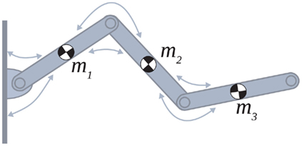
Figure 1. Schematic of the simulated biomechanical limb where each joint is flanked by an opposing pair of muscle actuators (arrows). Each limb segment was modeled as a long, thin, rigid body of length L_i and mass m_i.

Co-contraction (the simultaneous contraction of antagonist muscles) is known to stabilize limb movements (Milner and Cloutier, 1995; Milner, 2002; Zakotnik et al., 2006; Lametti et al., 2007) and is regarded as a distinct component of the motor command in many theoretical models of motor control (Feldman and Levin, 1995; Bhushan and Shadmehr, 1999; Gribble and Ostry, 1999; Todorov, 2000; Gribble, 2003; Neilson and Neilson, 2005). However traditional planar limb models typically lump opposing muscles into unitary joint actuators that do not accommodate co-contraction. The present model overcomes this limitation by actuating each joint with an antagonistic pair of muscle actuators that may be activated independently.

Co-contraction alters the biomechanical operating ranges of muscle and tendon by increasing both muscle damping (viscosity) and musculotendon stiffness (elasticity). Winters and Stark(1985, 1988) show that dynamic limb impedance (resistance to perturbation) is accurately predicted by an eighth-order model of antagonist Hill-based muscles. Such models (after Hill, 1938) include a series elastic (SE) element that represents the passive elasticity of muscle tissue and tendon (see Winters and Stark, 1987; Zajac and Winters, 1990; Pandy, 2001; Winter, 2005; Erdemir et al., 2007, for reviews). In these models the series elastic stiffness increases (becomes less compliant) non-linearly with stretch which results in increased joint stiffness under co-contraction (Winters et al., 1988).

Despite this, musculotendon series elasticity is typically an order of magnitude stiffer than contractile muscle tissue and we treat it as negligible in the present model. This simplification permits insights into the dynamics through a formal stability analysis, although it comes at the loss of co-contraction mediated changes in musculotendon stiffness. Nonetheless, the model retains sufficient kinematic realism to make it a useful platform for exercising neuromotor models of low to moderate speed movements where series elasticity has little impact.

In the present paper we derive the full biomechanical limb model followed by a numerical stability analysis of an isolated pair of antagonistic muscles using the method of numerical continuation. The stability analysis reveals the dynamic character of opponent muscles and illuminates the effects of co-contraction from a dynamical systems viewpoint. In particular, it reveals that strongly co-contracting muscles can exhibit multiple distinct stable (multistable) equilibrium positions depending on the biomechanical properties of the muscles involved. In biomechanical parlance, monostability satisfies equifinality whereby a limb always returns to same equilibrium position following a perturbation (Bizzi et al., 1978; Kelso and Holt, 1980; Schmidt et al., 1986; Feldman and Latash, 2005). We analytically derive the nullclines of the opponent muscle system and formally prove that monostability is guaranteed for the special case of opponent muscles with identical properties. Two numerical experiments are presented which validate these findings in the full biomechanical limb. Experiment 1 demonstrates the effects of co-contraction on limb damping and Experiment 2 demonstrates the emergence of multiple equilibrium postures with strong co-contraction.

Methods

Skeletal and musculotendon kinematics were modeled as a series of independent transforms following Zajac (1989) and Pandy (2001). The forward dynamics were implemented using the Newton-Euler method following Otten (2003). The muscle dynamics were implemented using the Voigt muscle model (Figure 2A) where the force-length and force-velocity properties of muscle tissue were approximated by simple mathematical forms (Figures 2B,C) that captured the general shape of curves reported in the physiological literature.

FIGURE 2

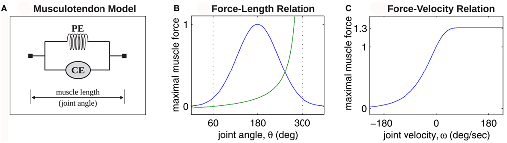
Figure 2. (A) Voigt model of muscle elasticity. Contractile element (CE) represents the lumped contraction forces of the muscle sarcomeres. Parallel elastic element (PE) represents the lumped elastic forces of muscle tissue. Series elasticity of muscle and tendon is assumed to be negligible and muscle length is considered a linear function of joint angle. (B) Force-length relationships for CE (blue line) with θ_min = 60°, θ₀ = 180°, θ_max = 300°, k_l = − (θ_max − θ₀)²/ln(0.1), and PE (green line) with k_pe = 0.1. Vertical axis is normalized with respect to F_max. (C) Force-velocity relationship for CE with k_v = 1. Maximal muscle force asymptotes at 1.313 F_max.

Contemporary models of forward dynamics are usually derived from the Lagrangian formulation of the overall energy in the system implemented using kinematic chains of rigid links (see Craig, 1989; Spong et al., 2006). However the equations of motion are typically non-trivial and are often derived using a symbolic algebra solver in practice (see Westervelt et al., 2007, for a modern tutorial on this approach). The Newton-Euler method, on the other hand, is the more straightforward approach for modeling small systems such as ours (Otten, 2003). Although it does suffer from the problem of numerical drift whereby rounding errors accumulate over time resulting in a slow dislocation of the limb joints. We therefore extended the method to incorporate spring-like binding forces within the limb joints to constrain numerical drift and maintain the geometric integrity of the limb over the long term (see Appendix B). It should be noted that contemporary methods using kinematic chains do not suffer from numerical drift so our solution does not apply to those methods.

Forward Dynamics of Skeletal Mechanics

Each limb segment was modeled as a long thin rigid body of mass m_i and length L_i where the subscript (i = 1, 2, 3) identifies the individual segments. The motion of the center of mass of each body was described by position angular orientation θ_i, translational velocity and angular velocity ω_i = dθ_i/dt.

The motions of all bodies were solved simultaneously according to the Newton-Euler method where Newton’s law,

governed the translational acceleration of each limb segment (treated as a point mass) in response to internal joint forces and , gravitational force and an external damping force Likewise Euler’s law,

governed the angular acceleration α_i = dω_i/dt of each limb segment (treated as a rigid body with moment of inertia ) in response to internal wrenching torques τ_Pi and τ_Qi as well as an external torque τ_Ei and a damping torque τ_Di = − k_τω_i.

Equations (1) and (2) were rearranged as a set of first-order ordinary differential equations and integrated numerically in MATLAB. Full details of the forward model are provided in Appendix A. Our extensions to the conventional method are presented in Appendix B. All parameters of the forward model are listed in Table 1.

TABLE 1

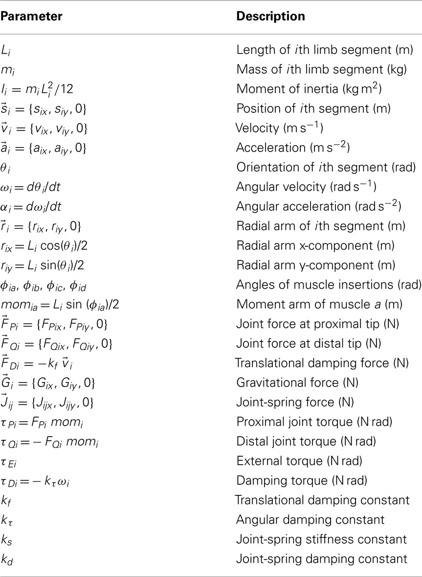
Table 1. Description of all parameters related to the forward dynamics.

Muscle Contraction Dynamics

Muscle was modeled by an active contractile element (CE) in parallel to a passive elastic element (PE) according to the Voigt model (Figure 2A). The net force imparted by the muscle was thus

where a(t) ∈ [0, 1] denotes the instantaneous level of muscle activation, F_max denotes maximal muscle force, denotes joint angle and denotes joint opening velocity. Muscle length was treated as a linear function of joint angle, as justified by cadaver studies (Grieve et al., 1978). Notice we use hat notation to distinguish joint angle and joint opening velocity from limb segment orientation θ and limb segment angular velocity ω.

The CE force-length relationship (blue line in Figure 2B) was modeled by a Gaussian curve,

centered on resting muscle length as is conventional (see Winters and Stark, 1987; Zajac, 1989). The PE force-length relationship (green line in Figure 2B) was approximated by a hyperbolic curve,

where and specified the limits of joint movement and the constant k_pe specified the slope. The CE force-velocity relationship (Figure 2C) was approximated by an exponential hyperbolic tangent,

with a single slope parameter, k_v, rather than piecewise hyperbolics after Hill (1938). See Table 2 for a list of all parameters related to muscle dynamics.

TABLE 2

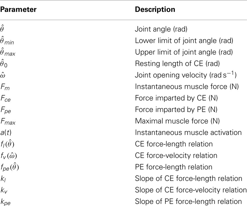
Table 2. Description of parameters related to muscle dynamics.

Stability Analysis of Opposing Muscles

We analyzed the angular motion of an isolated limb segment actuated by a pair of opposing muscles to gain insights into the effects of co-contraction. The muscles imposed opposing torques,

and

on the limb segment where F denotes contractile muscle force (3) and mom denotes the moment arm of the muscle. These torques were substituted into Euler’s law (2) and integrated numerically as a set of first-order ordinary differential equations.

The damping effects of co-contraction were investigated by comparing the motions of the isolated limb under differing conditions of muscle co-activation but identical net joint torques. Phase portraits of the motion (θ_a versus ω_a) were computed for conditions of nil muscle activation (a_a = a_b = 0), 25% muscle activation (a_a = a_b = 0.25), and 50% muscle activation (a_a = a_b = 0.5) where the latter represents the upper limit of co-contraction in physiological conditions. Each phase portrait portrays all possible motions of the limb segment for a given set of muscle activations. The flow of the vector field in the phase portrait can be characterized by the nullclines of the dynamic variables which corresponds to those cross sections through phase space where growth of one or more variables is zero. Equilibrium points occur where the nullclines intersect and the growth of all variables is zero. Linearizing the flow around equilibrium points allows their stability to be quantified by their eigenvalues. The real part of the eigenvalue quantifies the rate of convergence to the equilibrium point (damping) whereas the imaginary part of the eigenvalue quantifies the rotational component (oscillation frequency) of the vector field around the equilibrium point. When a parameter change causes the real part of the eigenvalue to cross zero from below, stability of the equilibrium point is lost as fluctuations grow exponentially. This is known as a local bifurcation of a continuous dynamical system and is classified as either a saddle-node, transcritical, pitchfork, or Hopf bifurcation according to the nature of the ensuing flow (see Strogatz, 2000; Breakspear and Jirsa, 2007, for reviews).

Preliminary analysis of these nullclines also suggested that gross asymmetries in the force-length properties of the opponent muscles may cause the equilibrium position of the joint to bifurcate into a co-existing pair of non-unique equilibrium positions under high levels of co-contraction. Phase portraits were thus computed for opponent muscles in which the resting length of the CE force-length property θ₀ had been shifted away from the midpoint of the muscle’s range of extension by the arbitrary amount of 1 rad under various conditions of balanced co-contraction (a_a = a_b) and imbalanced co-contraction (a_a varied while a_b held fixed). Parameter space was explored by numerical continuation of the observed bifurcation points was performed using the CL_MATCONT numerical toolkit (Dhooge et al., 2003).

Numerical Experiment 1: Effect of Co-Contraction on Damping

The effect of co-contraction mediated muscle damping was verified in the full biomechanical limb by comparing the motion of identical limbs under conditions of medium (near 20%), strong (near 50%), and extreme (near 80%) co-contraction (Table 3) with identical net muscle activations across conditions. Extreme co-contraction represents the theoretical limit of co-contraction in the mathematical sense and does not occur in nature. Muscle activations were held constant for the duration of the simulation (10 s) with the limb initially hanging at rest from the base pivot. All other parameters were held fixed (m_i = 1, L_i = 1, k_f = 0, k_τ = 0, k_s = 1, k_d = 1, G_ix = 0, G_iy = − 9.81, F_max,1 = 4000, F_max,2 = 2000, F_max,3 = 1000, k_pe = 0.1, k_l = − π²/ln(0.1), k_v = 0.2, ɸ_a = − 0.2, ɸ_b = 0.2, ɸ_c = 0.2, ɸ_d = − 0.2, θ_min = 0.3π, θ_max = 1.6π, θ₀ = 0.95π).

TABLE 3

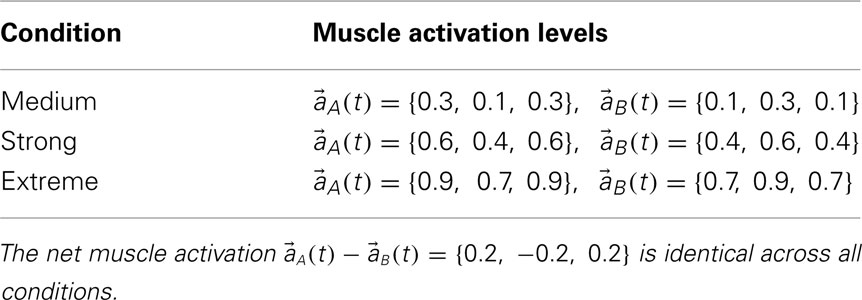
Table 3. Muscle activation levels for the conditions of medium, strong, and extreme co-contraction used in Experiments 1 and 2.

Numerical Experiment 2: Effect of Asymmetric Muscles

The effect of co-contraction mediated multistability in asymmetric muscles was verified in the full biomechanical limb model by comparing the final postures adopted (at t = 30 s) by n = 200 simulation runs of identical limbs undergoing medium, strong, and extreme co-contraction from random initial postures (always at rest). The same set of initial postures were used in both co-conditions and muscle asymmetries were imposed by shifting the CE resting length of opposing muscles to All other parameters were the same as those in Experiment 1.

Results

Stability Analysis of Opposing Muscles

Analysis of the isolated limb segment revealed co-contraction modulated muscle damping effects emerged natively from the muscle model. Furthermore, a wide range of muscle activations were found to yield bistable equilibria when the opponent muscles were configured with asymmetric CE force-length properties.

Figure 3 reveals the differing levels of damping exhibited by the isolated limb segment under conditions of 0, 25, and 50% co-contraction. Damping was entirely absent under 0% co-contraction (Figure 3A) as seen by the closed orbits around the equilibrium position. The lack of damping was confirmed quantitatively by noticing that the real part of the eigenvalues of the equilibrium position were zero (λ_1,2 = 0 ± 0.174i). By comparison, progressively more damping was observed in the 25% co-contraction (Figure 3B) and 50% co-contraction (Figure 3C) conditions, as quantified by progressively larger negative values in the real parts of the eigenvalues (λ_1,2 = − 0.0657 ± 0.161i and λ_1,2 = − 0.1314 ± 0.114i respectively).

FIGURE 3

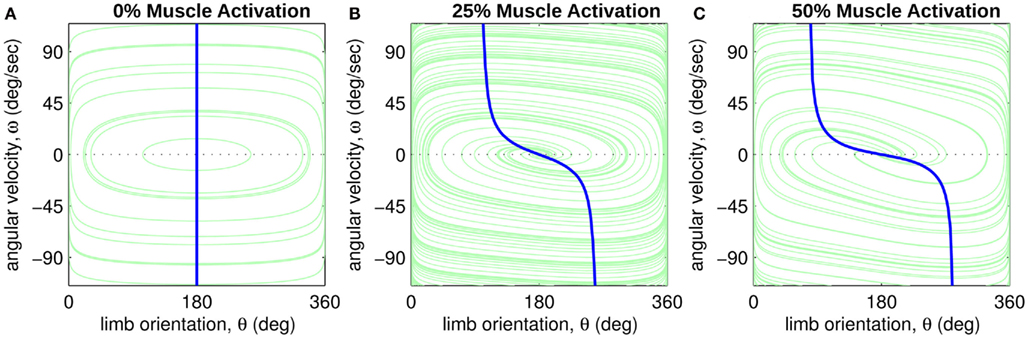
Figure 3. Phase portraits of the motion of an isolated limb segment actuated by an opposing pair of symmetric muscles under conditions of (A) nil co-activation (a_a = a_b = 0), (B) 25% co-activation (a_a = a_b = 0.25) and (C) 50% co-activation (a_a = a_b = 0.5). The latter approximates the biological limit of muscle co-contraction in nature. All other musculoskeletal parameters are identical in all three conditions (m = 5, L = 1, ɸ = 0.2, F_max = 1, k_l = −π²/In(0.1), k_v = 2, k_pe = 0.1, , , ). Horizontal axis in each panel represents the angular position of the limb segment (θ) and is synonymous with both joint angle and muscle length. Vertical axis represents the angular velocity of the limb segment (ω) and is synonymous with muscle lengthening velocity. Faint green lines indicate randomly selected motion trajectories. Heavy blue line in each panel indicates the nullcline of ω. Its zero-crossings denote the equilibrium positions of the limb segment (θ = 180 degrees in all panels). The curvature of the nullcline qualitatively characterizes the degree of damping in the vector field. Damping is also quantified by the eigenvalues at the equilibrium point (see text) which confirm that damping is absent under nil co-activation and increases with higher levels of co-activation.

Figure 4A reveals the existence of bistable equilibrium positions in the same joint when the muscles were configured with asymmetric CE force-length properties (θ_a0 = θ_b0 = π − 1) and subjected to 50% co-contraction. Since the nullcline of is always in the present model, we need only consider the nullcline of to understand the motion of the joint. Figure 4B shows the nullclines for the asymmetrically actuated limb under differing levels of balanced co-contraction (a_a = a_b = 0, …, 1). It reveals a supercritical pitchfork bifurcation in the equilibrium positions as co-contraction exceeds the critical value of a_a = a_b = 0.17 (indicated by the branch point BP). The pitchfork bifurcation occurs when the slope of the nullcline at the central stable equilibrium point changes sign resulting in a nullcline with three distinct zero crossings. In the supercritical case, these three zero crossings correspond to a central unstable equilibrium point flanked by a pair of stable equilibrium points.

FIGURE 4

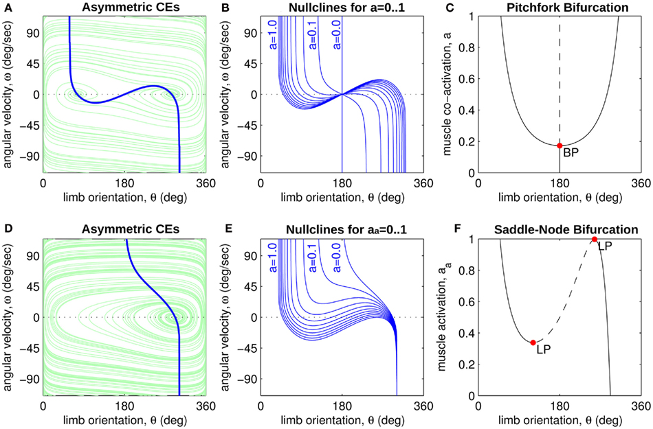
Figure 4. (A) Phase portrait of an isolated limb segment actuated by opposing muscles with asymmetric CE force-length properties at 50% co-activation (a_a = a_b = 0.5). All other parameters are identical to those of Figure 3. One unstable equilibrium point is observed at and two stable equilibrium points are observed at and respectively. (B) Nullclines for the same limb segment after manipulating muscle co-activation (a = a_a = a_b) from 0 to 1 in steps of 0.1. (C) Bifurcation plot showing the onset of bistability in the equilibrium positions through a pitchfork bifurcation as muscle co-activation is increased. Solid lines indicate stable equilibrium points, dashed lines indicate unstable equilibrium points. The branch point (BP) marks the onset of bistability (a = 0.172). (D) Same as (A) except here a_a = 0., a_b = 0.5 and only a single stable equilibrium point (þeta = 292°) is observed. (E) Same as (B) except here a_b = 0.5 is held fixed while a_a is manipulated from 0 to 1. (F) Bifurcation plot showing the emergence of bistability through a saddle-node bifurcation as muscle activation a_a is increased while a_b = 0.5 is held fixed. The limit points (LP) mark the onset (a_a = 0.338) and offset (a_a = 0.998) of bistability.

Similarly, Figures 4D–F describe the motion of the asymmetrically actuated limb when a_b = 0.5 is held fixed while a_b is manipulated. Here we observe a saddle-node bifurcation that yields bistable equilibrium positions when muscle activations are within the critical range 0.338 < a_a < 0.998. The saddle-node (or fold) bifurcation occurs when the turning points in the nullcline fold back far enough to support multiple zero crossings, specifically, one unstable equilibrium flanked by two stable equilibria.

Figure 5A shows the bistability map for the asymmetric joint with θ₀ = π − 1. It reveals the extent of muscle activations that yield bistable equilibrium positions in this case. The cusp point (CP) corresponds to the branch point in Figure 4C and it marks the furthest extent of the bistable region. Its position (always on the line a_a = a_b) depends upon the CE resting length parameter θ₀. Figure 5B plots the migration of the cusp point as θ₀ is manipulated. Here we see that the bistability emerges at 100% co-contraction levels when θ₀ = 3.00 rad (point A) while it emerges at 50% co-contraction levels when θ₀ = 2.86 rad (point B). Bistability therefore emerges in the biological operating range of co-contraction when the CE resting lengths of the opposing muscles are shifted away from the muscle midpoint by as little as (π − 2.86) radians (16.1°).

FIGURE 5

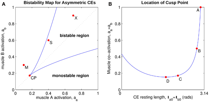
Figure 5. (A) Bistability map for the isolated limb segment with asymmetric CE force-length properties (θ₀ = π − 1). Solid lines indicate the transition boundary between bistable and monostable regions. Dotted line indicates balanced co-contraction (a_a = a_b). Cusp point (CP) marks the furthest extent of the bistable region (a_a = a_b = 0.171). Points M, S, and X correspond to the conditions of medium, strong, and extreme co-contraction applied in Experiments 1 and 2. (B) Shows the migration of the cusp point along the line of balanced co-contraction when the CE resting length parameter is manipulated between θ₀ = θ_a0 = θ_b0 = 0 (the limit of joint flexion) and θ₀ = θ_a0 = θ_b0 = π (the midpoint of muscle). Point A (θ₀ = 3.00, a = 1) marks the emergence of bistability at 100% co-contraction levels. Point B (θ₀ = 2.86, a = 0.5) marks the emergence of bistability at 50% co-contraction levels. Point C (θ₀ = π − 1, a = 0.171) corresponds to point CP in the previous panel. Point D (θ₀ = 1.68, a = 0.154) marks the maximal extent of the bistable region.

In comparison, bistability emerges at 17.1% co-contraction levels when θ₀ = π − 1 (point C) which is the value used in our simulations. This happens to be close to the maximal extent of bistability which emerges at only 15.4% co-contraction levels when θ₀ = 1.68 rad (point D) and corresponds to shifting θ₀ by (π − 1.68) radians (83.7°) from the muscle midpoint – which is an extreme shift.

Numerical Experiment 1

Co-contraction modulated damping effects were confirmed in the full biomechanical limb. Figures 6A–C show the trajectories of the limb under conditions of medium, strong, and extreme co-contraction. Figure 6D tracks the vertical position of the limb tip for each condition where limb damping is observed to increase with higher levels of co-contraction. The limb converged to the same equilibrium position in all conditions, confirming that multistability did not apply when the opponent muscles were symmetrically matched.

FIGURE 6

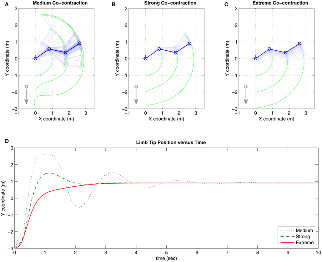
Figure 6. Results of Numerical Experiment 1. (A–C) Show the trajectories of the full biomechanical limb under conditions of medium, strong, and extreme co-contraction in the presence of gravity (denoted by G). Here, medium contraction is close to 20% activation capacity. Strong co-contraction is close to 50% capacity and thus approximates the biological limit of co-contraction. Extreme co-contraction is close to 80% capacity and approximates the mathematical limit of co-contraction. Limb position is sampled at 0.1 s intervals in all three panels. (D) Tracks the vertical position of the limb tip for each co-contraction condition. Damping in the full biomechanical limb is observed to increase with higher levels of co-contraction, consistent with the findings for the isolated limb segment. See Movie S1 in Supplementary Material for an animated version of this figure.

Numerical Experiment 2

Co-contraction modulated multistability was confirmed in the full biomechanical limb with asymmetric CE force-length properties. Figure 7A shows the random initial limb postures used in all conditions. Figures 7B–D show the final limb postures for medium, strong, and extreme co-contraction respectively. All limbs undergoing medium co-contraction converged to the same posture (Figure 7B) and are indistinguishable. In contrast, limbs undergoing extreme co-contraction (Figure 7D) converged to one of six distinct stable postures which clearly demonstrated that all joints were operating in the bistable regime, whereas limbs undergoing strong co-contraction (Figure 7C) converged to one of only two distinct equilibrium postures. Nonetheless, all joint angles in this condition diverged noticeably from those observed under medium co-contraction suggesting all were operating in the bistable regime even though only some had converged to distinct equilibrium positions.

FIGURE 7

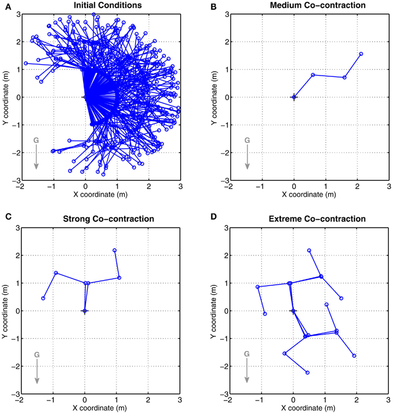
Figure 7. Results of Numerical Experiment 2. (A) Shows the random initial limb postures for all simulation runs (n = 200) of the full biomechanical limb. (B–D) Show the final limb postures adopted by all runs under conditions of medium, strong, and extreme co-contraction respectively. Opposing muscles have asymmetric CE force-length properties (θ_a0 = θ_b0 = π − 1) otherwise all parameters are the same as Figure 6. All limbs undergoing medium co-contraction converged to same final posture whereas those undergoing strong and extreme co-contraction converged to non-unique final postures. These observations are consistent with the findings of bistability in the isolated limb segment. See Movie S2 in Supplementary Material for an animated version of this figure.

Not all of the possible combinations of (bi)stable joint solutions yield stable limb postures in Figures 7C,D. This is particularly noticeable in Figure 7D where two of the eight possible postural combinations of bistable joints are rendered unstable by the action of gravity. Critical slowing of the limb is evident in the vicinity of these “missing” postures (see Movie S2 in Supplementary Material) confirming that the system is close to a stable regime even though stability is not achieved in this case.

Conditions for Monostability

By dynamical system theory the limb joint is guaranteed to be monostable when the velocity nullcline is monotonically decreasing and thus has only one zero-crossing (as is the case in Figure 3). Here, we derive an analytical expression for the equilibrium position of the isolated limb segment for the special case of identical antagonist muscles. We then use that expression to prove that monostability is guaranteed in the special case. This proof does not preclude the possibility that monostability may also hold when antagonistic muscles are similar but not identical.

The equilibrium position of the limb segment is given by the intersection of the nullclines of and but since the nullcline of is always for our system we need only consider the zero crossings of the nullcline of Solving Euler’s law of motion for the case where and substituting muscle equations (3–6) allows the nullcline to be expressed as

where

are defined for brevity. Observe that at the zero crossings of (9) and all force-velocity relations have f_v(0) = 1 by definition thus the zero crossings of the nullcline are obtained by solving the expression

where θ_a + θ_b = 2π. We now use this expression to prove the following theorem.

Theorem. The nullcline (9) of an isolated limb segment actuated by an identical pair of opposing Voigt muscles always has exactly one root for any given pair of fixed muscle activations, a_a and a_b. Thus monostability of the limb segment is guaranteed for all possible muscle activations.

PROOF. The roots of nullcline (9) are given by equation (10). When the opponent muscles (denoted “a” and “b”) have identical muscuoloskeletal properties (mom_a = mom_b, F_max,a = F_max,b, k_la = k_lb, k_pea = k_peb, ) then equation (10) reduces to

where can be expressed in terms of by substituting as follows,

Similarly, can be expressed in terms of by substituting as follows,

Substituting (12) and (13) into (11) yields

where

and

are defined for convenience. From this point onward we omit the muscle subscript (a) from the notation for brevity. Notice that corresponds to a Gaussian curve centered on with a peak amplitude of (a_a − a_b)/k_pe. Notice also that corresponds to the difference of two hyperbolics which asymptotes vertically to +∞ at and to −∞ at with a zero crossing at Functions and are both continuous on the interval

We argue geometrically that functions and always intersect exactly once on the interval for any value of (a_a − a_b) and therefore equation (11) always has exactly one solution. It follows from the definition of (11) that nullcline (9) always has exactly one root when the opposing muscles are symmetric.

Case 1: a_a = a_b

Here thus equation (14) reduces to

which simplifies to the unique solution

after rearranging and canceling redundant terms. Thus nullcline (9) has exactly one root when a_a = a_b.

Case 2: a_a > a_b

Here is a continuous, non-negative function that is monotonically increasing on the interval and monotonically decreasing on the interval whereas is a continuous, monotonically decreasing function that is non-negative on the interval and non-positive on the interval

Since and are both non-negative in the interval wherein is monotonically increasing and is monotonically decreasing from its upper bound of +∞ to its lower bound of zero then there must exist exactly one solution in where is satisfied.

On the other hand, is always positive and is always non-positive on the interval Hence there are no solutions in this interval that satisfy Consequently, exactly one solution to equation (14) exists in this case across the entire interval Thus nullcline (9) has exactly one root when a_a > a_b.

Case 3: a_a < a_b

Similar to case 2 except here is a continuous, non-positive function that is monotonically decreasing on the interval and monotonically increasing on the interval whereas is unchanged.

Following the same reasoning as above, no solutions to exist in the interval and exactly one solution exists in the interval Consequently, exactly one solution to equation (11) exists in this case across the entire interval Thus nullcline (9) has exactly one root when when a_a < a_b.

Discussion

Our objective was to provide a simplified anatomical forward model of limb movement that replicates the fundamental dynamical relationships between muscle co-contraction and limb movement. Limb anatomy was reduced to a planar three-link rigid body limb where each joint is actuated by an opposing pair of simplified muscle actuators having force-length-velocity properties that approximate those of natural muscle systems. Stability analysis of a pair of antagonist muscle actuators confirmed that co-contraction increases muscle damping as anticipated. The stability analysis also revealed that co-contraction induces bistable equilibrium when the force-length properties of the opponent CEs are sufficiently asymmetric. Both findings were verified in the full biomechanical limb model where overall limb damping increased with co-contraction (Numerical Experiment 1) and multiple co-existing stable equilibrium postures were evoked when co-contraction was high (Numerical Experiment 2).

The effect of co-contraction on muscle damping is best understood by inspecting equation (3) of the muscle model and observing that muscle activation a(t) modulates both the force-length and force-velocity properties of the contractile element. Muscle activation therefore modulates both isometric muscle force and muscle damping to the same extent however the opposing isometric muscle forces cancel to produce nil joint torque whereas the damping forces of both muscles unite against the common muscle movement.

On the other hand, the effect of co-contraction on joint stability is best understood in terms of the velocity nullcline for a single pair of opposing muscles. Increased co-contraction induces turning points in the velocity nullcline when the force-length curves of the opponent muscles are sufficiently asymmetric. Above a critical level of co-contraction these turnings can become large enough for the nullcline to support multiple zero crossings. In such cases, the unique stable equilibrium bifurcates to yield a pair of non-identical stable equilibria. The critical level of co-contraction at which bistability emerges is determined by the degree of asymmetry in the force-length properties of the antagonist muscles. Bistability does not emerge when the antagonist muscles have identical properties.

Implications for Motor Control Theory

While co-contraction is known to modulate both muscle damping and musculotendon stiffness, it has not previously been implicated with bistable equilibria to the best of our knowledge. Indeed, mainstream theoretical accounts of biological motor control (e.g. Feldman, 1966; Feldman and Levin, 1995) typically assume that co-activations of antagonist muscles implicitly translate into monostable equilibrium positions. However our findings suggest that such an assumption may not always be justified. Existing theoretical accounts may therefore need to accommodate the additional complexities of either controlling or avoiding bistability in the muscle apparatus to achieve unambiguous forward control of the joint.

Whether co-contraction mediated bistability occurs in nature remains an open question. Our analysis suggests that bistable postures can emerge at biologically plausible levels of co-contraction (50% maximal isometric force) when the CE resting length parameters are offset from the muscle midpoint by as little as 16.1°. This critical offset value corresponds to a peak-to-peak discrepancy in the force-length curves of the antagonist muscles of 32.2° (twice the offset). This critical value happens to be exceeded by the peak-to-peak discrepancies in human elbow (40°), knee (40°), and ankle (60°) reported by Winters and Stark (1985). So it is not unreasonable to consider that bistable antagonist muscle systems may indeed exist in nature.

Implications for Neurorobotics

The increasing use of biomimetic actuators in robotic systems (e.g. Ayers et al., 2002; Safak and Adams, 2002) complements the neurorobotic doctrine that the brain cannot be studied separately from the body (Chiel and Beer, 1997). The central nervous system’s ability to use muscle co-contraction to actively control limb damping highlights the tight integration between the functionality of the motor control system and the contractile dynamics of muscle tissue. However not all muscle properties have equivalent functional relevance to the motor control system so only the most relevant muscle properties need be incorporated into biomimetic actuators.

Our biomechanical model demonstrates that simplified actuators with idealized forms of CE force-length-velocity properties are sufficient to permit active control of joint damping through co-contraction. More specifically, it is crucial that the force-velocity property of the actuator be modulated by its activation level for co-contraction modulated damping effects to occur. Musculotendon series elasticity, for example, is not necessary for this purpose. As we have shown, care must be taken with the force-length property of the actuator to avoid gross non-linearities in the dynamics of opposing actuators which can introduce non-unique equilibria into the forward dynamics that merely complicate the problem of joint control. Thankfully, numerical stability analysis allows the monostable operating limits of antagonist actuators to be ascertained from the contractile dynamics of a single biomimetic actuator.

Limitations

The contractile dynamics of the present biomechanical model were simplified by the use of the Voigt muscle model which lacks a series elastic element. This simplification made it possible to derive an analytical solution to the equilibrium position of antagonist muscles and to prove that monostability is guaranteed for identical muscles. However musculotendon series elasticity is known to have a significant impact on muscle stiffness during rapid movement (Winters and Stark, 1985; Winters et al., 1988). The physiological accuracy of the present model is therefore limited to low and moderate speed movements where dynamic changes in muscle stiffness are negligible.

Conclusion

Our analysis of antagonistic Voigt muscles highlights that even simple muscle systems can exhibit unexpected multistable behaviors. Insights into these complex behaviors were gleaned through the application of formal methods from dynamical system theory where knowledge of the nullclines of the dynamic variables allowed us to predict the stability of the equilibrium positions of co-contracting muscles and to map the conditions under which co-contraction induces bistable joint postures. Bistability complicates the problem of achieving unambiguous control over the forward dynamics. Its existence has practical implications for the design of non-linear biomimetic actuators and theoretical implications for accounts of biological motor control that presume antagonist muscle systems are universally monostable. Further numerical analysis using more elaborate antagonist muscle models is required to assess the impact of musculotendon series elasticity on the emergence of bistability. Empirical research is ultimately required to establish whether bistable antagonist muscle dynamics can be observed in nature.

Conflict of Interest Statement

The authors declare that the research was conducted in the absence of any commercial or financial relationships that could be construed as a potential conflict of interest.

Acknowledgments

We gratefully acknowledge the financial support provided by the Australian Government (ARC Thinking Systems Grant TS0669860), Brain Sciences UNSW, and the Black Dog Institute. NF also acknowledges the financial support of Fonds Québécois de la Recherche sur la Nature et les Technologies (FQRNT). We also thank Dr Tjeerd Boonstra for his valuable comments and suggestions.

Supplementary Material

The Movies S1 and S2 for this article can be found online at http://www.frontiersin.org/neurorobotics/10.3389/fnbot.2011.00005/abstract

Footnotes

1. ^LifeMOD is a registered trademark of Biomechanics Research Group, Inc.
2. ^The MATLAB source code is available from the authors on request. MATLAB is a registered trademark of The Mathworks, Inc.

References

Ayers, J., Davis, J., and Rudolph, A. (2002). Neurotechnology for Biomimetic Robots. Cambridge: The MIT Press.

Bhushan, N., and Shadmehr, R. (1999). Computational nature of human adaptive control during learning of reaching movements in force fields. Biol. Cybern. 81, 39–60.

Pubmed Abstract | Pubmed Full Text | CrossRef Full Text

Bizzi, E., Dev, P., Morasso, P., and Polit, A. (1978). Effect of load disturbances during centrally initiated movements. J. Neurophysiol. 41, 542.

Pubmed Abstract | Pubmed Full Text

Breakspear, M., and Jirsa, V. (2007). “Neuronal dynamics and brain connectivity,” in Handbook of Brain Connectivity, Volume 12 of Understanding Complex Systems, eds V. Jirsa and A. McIntosh (Berlin: Springer), 3–64.

Chiel, H., and Beer, R. (1997). The brain has a body: adaptive behavior emerges from interactions of nervous system, body and environment. Trends Neurosci. 20, 553–557.

Pubmed Abstract | Pubmed Full Text | CrossRef Full Text

Conforto, S., Bernabucci, I., Severini, G., Schmid, M., and D’Alessio, T. (2009). Biologically inspired modelling for the control of upper limb movements: from concept studies to future applications. Front. Neurorobotics 3:3. doi:10.3389/neuro.12.003.2009

CrossRef Full Text

Craig, J. (1989). Introduction to Robotics: Mechanics and Control, Vol. 74. New York: Addison-Wesley.

Dhooge, A., Govaerts, W., Kuznetsov, Y., Mestrom, W., and Riet, A. (2003). “CL_MATCONT: a continuation toolbox in matlab,” in Proceedings of the 2003 ACM Symposium on Applied Computing, New York, 161–166.

Erdemir, A., McLean, S., Herzog, W., and van den Bogert, A. J. (2007). Model-based estimation of muscle forces exerted during movements. Clin. Biomech. (Bristol, Avon) 22, 131–154.

Pubmed Abstract | Pubmed Full Text | CrossRef Full Text

Feldman, A. (1966). Functional tuning of the nervous system with control of movement or maintenance of a steady posture. II. Controllable parameters of the muscle. Biophysics 11, 565–578.

Feldman, A. G., and Latash, M. L. (2005). Testing hypotheses and the advancement of science: recent attempts to falsify the equilibrium point hypothesis. Exp. Brain Res. 161, 91–103.

Pubmed Abstract | Pubmed Full Text | CrossRef Full Text

Feldman, A. G., and Levin, M. F. (1995). The origin and use of positional frames of reference in motor control. Behav. Brain Sci. 18, 723–744.

CrossRef Full Text

Gribble, P. L. (2003). Role of cocontraction in arm movement accuracy. J. Neurophysiol. 89, 2396–2405.

Pubmed Abstract | Pubmed Full Text | CrossRef Full Text

Gribble, P. L., and Ostry, D. J. (1999). Compensation for interaction torques during single-and multijoint limb movement. J. Neurophysiol. 82, 2310.

Pubmed Abstract | Pubmed Full Text

Grieve, D. W., Pheasant, S., and Cavanagh, P. R. (1978). “Prediction of gastrocnemius length from knee and ankle joint posture,” in Biomechanics VI: Proceedings of the Sixth International Congress of Biomechanics (Copenhagen: University Park Press), 405.

Harischandra, N., Cabelguen, J., and Ekeberg, O. (2010). A 3D Musculo-Mechanical model of the salamander for the study of different gaits and modes of locomotion. Front. Neurorobotics. 4:112. doi:10.3389/fnbot.2010.00112

CrossRef Full Text

Hill, A. V. (1938). The heat of shortening and the dynamic constants of muscle. Proc. R. Soc. Lond. B Biol. Sci. 126, 136–195.

CrossRef Full Text

Kelso, J., and Holt, K. (1980). Exploring a vibratory systems analysis of human movement production. J. Neurophysiol. 43, 1183.

Pubmed Abstract | Pubmed Full Text

Lametti, D. R., Houle, G., and Ostry, D. J. (2007). Control of movement variability and the regulation of limb impedance. J. Neurophysiol. 98, 3516–3524.

Pubmed Abstract | Pubmed Full Text | CrossRef Full Text

Milner, T. (2002). Adaptation to destabilizing dynamics by means of muscle cocontraction. Exp. Brain Res. 143, 406–416.

Pubmed Abstract | Pubmed Full Text | CrossRef Full Text

Milner, T. E., and Cloutier, C. (1995). “The effect of antagonist muscle co-contraction on damping of the wrist joint during voluntary movement,” in IEEE 17th Annual Conference Engineering in Medicine and Biology Society, New York, Vol. 2.

Neilson, P. D., and Neilson, M. D. (2005). An overview of adaptive model theory: solving the problems of redundancy, resources, and nonlinear interactions in human movement control. J. Neural Eng. 2:S279–312.

Pubmed Abstract | Pubmed Full Text | CrossRef Full Text

Otten, E. (2003). Inverse and forward dynamics: models of multi-body systems. Philos. Trans. R Soc. Lond. B Biol. Sci. 358, 1493–1500.

Pubmed Abstract | Pubmed Full Text | CrossRef Full Text

Pandy, M. G. (2001). Computer modeling and simulation of human movement. Annu. Rev. Biomed. Eng. 3, 245–273.

Pubmed Abstract | Pubmed Full Text | CrossRef Full Text

Schmidt, R., McGown, C., Quinn, J., and Hawkins, B. (1986). Unexpected inertial loading in rapid reversal movements: violations of equifinality. Hum. Mov. Sci. 5, 263–273.

CrossRef Full Text

Spong, M., Hutchinson, S., and Vidyasagar, M. (2006). Robot Modeling and Control. Hoboken, NJ: John Wiley & Sons.

Strogatz, S. (2000). Nonlinear Dynamics and Chaos: With Applications to Physics, Biology, Chemistry, and Engineering. Boulder: Westview Press.

Todorov, E. (2000). Direct cortical control of muscle activation in voluntary arm movements: a model. Nat. Neurosci. 3, 391–398.

Pubmed Abstract | Pubmed Full Text | CrossRef Full Text

Todorov, E. (2004). Optimality principles in sensorimotor control (review). Nat. Neurosci. 7, 907.

Pubmed Abstract | Pubmed Full Text | CrossRef Full Text

Westervelt, E., Grizzle, J., Chevallereau, C., Choi, J., and Morris, B. (2007). Feedback Control of Dynamic Bipedal Robot Locomotion. Boca Raton: CRC Press.

Winter, D. A. (2005). Biomechanics and Motor Control of Human Movement, 3rd Edn. Hoboken, NJ: John Wiley & Sons.

Winters, J., and Stark, L. (1985). Analysis of fundamental human movement patterns through the use of in-depth antagonistic muscle models. IEEE Trans. Biomed. Eng. 826–839.

Pubmed Abstract | Pubmed Full Text | CrossRef Full Text

Winters, J., and Stark, L. (1987). Muscle models: what is gained and what is lost by varying model complexity. Biol. Cybern. 55, 403–420.

Pubmed Abstract | Pubmed Full Text | CrossRef Full Text

Winters, J., and Stark, L. (1988). Estimated mechanical properties of synergistic muscles involved in movements of a variety of humans joints. J. Biomech. 21, 1027–1041.

Pubmed Abstract | Pubmed Full Text | CrossRef Full Text

Winters, J., Stark, L., and Seif-Naraghi, A. H. (1988). An analysis of the sources of musculoskeletal system impedance. J. Biomech. 21, 1011–1025.

Pubmed Abstract | Pubmed Full Text | CrossRef Full Text

Zajac, F., and Winters, J. (1990). “Modeling musculoskeletal movement systems: joint and body segmental dynamics, musculoskeletal actuation, and neuromuscular control,” Multiple Muscle Systems: Biomechanics and Movement Organization (New York: Springer-Verlag), 121–148.

Zajac, F. E. (1989). Muscle and tendon: properties, models, scaling, and application to biomechanics and motor control. Crit. Rev. Biomed. Eng. 17, 359–411.

Pubmed Abstract | Pubmed Full Text

Zakotnik, J., Matheson, T., and Durr, V. (2006). Co-Contraction and passive forces facilitate load compensation of aimed limb movements. J. Neurosci. 26, 4995–5007.

Pubmed Abstract | Pubmed Full Text | CrossRef Full Text

Safak, K., and Adams, G. (2002). Modeling and simulation of an artificial muscle and its application to biomimetic robot posture control. Rob. Auton. Syst. 41, 225–243.

CrossRef Full Text

Appendix A

Derivation of the Forward Dynamics

Equations (1) and (2) can be rearranged as a set of first-order ordinary differential equations,

and integrated numerically to obtain the evolution of each limb segment’s position orientation θ_i, translational velocity and angular velocity ω_i from a given set of initial conditions

By convention, the system of equations (A1–A4) is closed by joint constraints that enforce matched accelerations of adjoining limb segments (i and j), namely

where represents the acceleration of the distal tip of the ith limb segment and represents the acceleration of the proximal tip of the jth limb segment (j = i + 1). The vectors and denote the proximal and distal radial arm vectors of the ith segment

So-called contact constraints similarly clamp the acceleration of the contact point with the external world to zero, namely

Equations (A5) and (A6) can be expanded to yield the constraints in the form of ordinary differential equations,

that are compatible with equations (A1–A4). Here i = 0, 1, 2 and j = i + 1 with individual terms having i = 0 being ignored.

Following Otten (2003), the unknown internal joint forces in equation (A3) were solved at each step of the integration by expressing equations (A3, A4, A7, A8) in matrix form AX = B and computing the inverse X = A^−1B where X represents the unknowns. Specifically,

where

and

See Table 1 for descriptions of all parameters.

Musculoskeletal Mechanics

Muscle paths were assumed to project linearly from attachment sites located at the midpoint of each limb segment and follow an approximately circular path around the joint shell. The transformation of muscle contraction force F to joint torque τ,

is determined exclusively by the moment arm (mom) of the joint reaction force. The joint reaction force is equal and opposite to the muscle contraction force and its moment arm was a fixed property of the limb anatomy, namely mom = (1/2)L sin(ɸ) where ɸ denotes the angle of insertion of the muscle line-of-action at the attachment site and denotes the limb segment’s radial arm vector.

Each limb segment had four muscle insertions (denoted a,b,c,d) where insertions a and b were connected to the opposing muscles of the proximal joint respectively and insertions c and d were connected to the opposing muscles of the distal joint. The net torque on the limb segment due to all four muscle torques was thus

where the torques τ_c and τ_d have negative sign because the radial arm vector to the distal joints has opposite direction to that of the proximal joint Substituting τ_net directly into the forward model of the skeleton as an external torque (τ_E in equation A9) enables the muscles to drive the skeleton and thus completes the forward model.

Appendix B

Constraining Numerical Drift

The conventional implementation of the Newton-Euler method (Appendix A) is prone to numerical drift whereby accumulated rounding errors lead to a slow dislocation of the joints over time. We overcame this problem by introducing small spring forces in the joints (Figure A1) that explicitly bound adjoining limb segments together and counteracted any dislocation as it occurred. Numerical error was thus constrained to the legal degrees of freedom of the limb in a manner that is commensurate with the connective tissues in biological joints however these joint forces are not proposed as models of the connective tissues per se.

Joint-springs (our terminology) were modeled as a damped linear spring suspended between two point masses representing the limb segments. Each joint-spring exerted a binding force of

on the tips of the adjacent limbs segments (i and j), where constant k_s denotes the stiffness of the joint-spring and k_d is the spring damping constant. By Newton’s law, this binding force induces an acceleration of at the tip of the proximal limb segment (Q1 in Figure A1) and an acceleration of at the tip of the distal limb segment (P2 in Figure A1).

These joint binding forces were incorporated into the forward model by relaxing the conventional joint constraint (A5) to accommodate the correcting accelerations induced by the joint-springs, namely

Likewise for the contact constraint (A6) which was redefined as

Notice these revised constraints are equivalent to the conventional constraints when the joint-spring accelerations and are zero. Equations (A13) and (A14) were incorporated into equation (A9) by redefining the coefficients

Pilot studies revealed that joint-springs were highly effective at preventing the dislocation of limb joints over time with 95.9% of joint gaps (sampled every 0.01 s) in 24 h of simulated limb motion being less than 1 mm.

FIGURE A1

Figure A1. Adjoining limb segments were bound at the joints by damped spring forces that counteracted numerical drift in the Newton-Euler method. The joint-spring shown here exerts a binding force of Newtons at point Q1 and an equal and opposite force on point P2. The magnitude of the spring force J is proportional to size of the joint gap. Similarly, the magnitude of the damping force (not shown) is proportional to the rate at which of the joint gap changes.