Statistical Phylogenetic Tree Analysis Using Differences of Means

We propose a statistical method to test whether two phylogenetic trees with given alignments are significantly incongruent. Our method compares the two distributions of phylogenetic trees given by two input alignments, instead of comparing point estimations of trees. This statistical approach can be applied to gene tree analysis for example, detecting unusual events in genome evolution such as horizontal gene transfer and reshuffling. Our method uses difference of means to compare two distributions of trees, after mapping trees into a vector space. Bootstrapping alignment columns can then be applied to obtain p-values. To compute distances between means, we employ a “kernel method” which speeds up distance calculations when trees are mapped in a high-dimensional feature space, e.g., splits or quartets feature space. In this pilot study, first we test our statistical method on data sets simulated under a coalescence model, to test whether two alignments are generated by congruent gene trees. We follow our simulation results with applications to data sets of gophers and lice, grasses and their endophytes, and different fungal genes from the same genome. A companion toolkit, Phylotree, is provided to facilitate computational experiments.

Introduction

Estimating differences between phylogenetic trees is one of the fundamental questions in computational biology. Conflicting phylogenies arise when, for example, different phylogenetic reconstruction methods are applied to the same data set, or even with one reconstruction method applied to multiple different genes. Gene phylogenies may be codivergent by virtue of congruence (identical trees) or insignificant incongruence. Otherwise, they may be significantly incongruent Maddison (1997). All of these outcomes are fundamentally interesting. Congruence of gene trees (or subtrees) is often considered the most desirable outcome of phylogenetic analysis, because such a result indicates that all sequences in the clade are orthologs (homologs derived from the same ancestral sequence without a history of gene duplication or lateral transfer), and that discrete monophyletic clades can be unambiguously identified, perhaps supporting novel or previously described taxa. In contrast, gene trees that are incongruent are often considered problematic because the precise resolution of speciation events seems to be obscured. Thus, it would also be very useful to identify significant incongruencies in gene trees because these represent non-canonical evolutionary processes (e.g., Maddison and Knowles, 2006; Edwards et al., 2007; Liu et al., 2008). In this paper we propose a statistical hypothesis test which tells whether two phylogenetic trees are significantly incongruent to each other by comparing two distributions for phylogenetic trees, instead of comparing two point estimations. More specifically we will compare two distributions of trees using difference of means. Our statistical hypotheses are:

H₀: Phylogenetic trees T₁ and T₂ are congruent.

H₁: Phylogenetic trees T₁ and T₂ are incongruent.

Usually a statistical test on the above hypotheses considers point estimates of the trees obtained by a tree reconstruction method, such as maximum likelihood (ML) estimates (Felsenstein, 1981; Galtier et al., 2005) or the neighbor-joining method (Saitou and Nei, 1987). See Schardl et al. (2008) and references within for an overview. Variation of reasonable tree estimates can be assessed, for example, by using the bootstrap or jackknife method.

There are several techniques to test if gene trees are codiverged. For example, the Bayesian estimation methods (e.g., Ane et al., 2007; Edwards et al., 2007; Liu and Pearl, 2007), the Templeton test implemented in paup* (Swofford, 1998; e.g., Ge et al., 1999), the partition-homogeneity test (PHT) also implemented in paup* (e.g., Voigt et al., 1999), Kishino–Hasegawa (KH) test (Kishino and Hasegawa, 1989), Shimodaira–Hasegawa (SH) test (Shimodaira and Hasegawa, 1999), and the likelihood ratio test (LRT; e.g., Vilaa et al., 2005) are statistical methods to see if there is a “significant” level of incongruence between the trees [these methods are also called partition likelihood support (PLS; Lee and Hugall, 2003)]. However, there is a limitation in many methods for comparing two phylogenetic trees: It is implicitly assumed that the two given trees are actually correctly estimated phylogenies. In reality, trees are estimated from observed data (e.g., fossil record, sequence data), and tree uncertainty is the rule instead of the exception. Holmes (2005) summarized a framework for statistical hypothesis testing on trees, including methods using distributions of phylogenetic trees, such as posterior distribution or bootstrap sampling distribution of trees. Holmes (2005) briefly described a statistical method to compare two bootstrap sampling distributions trees, using the mean and variance of each distribution. Here we expand these methods to use posterior means, instead of tree-valued tree estimators, to estimate trees. We propose using posterior means to estimate trees, and we apply the bootstrap method to assess variation in the posterior means.

This paper is organized as follows: In Section “Materials and Methods,” we state our method. In Section “Results,” we show simulation studies with data generated by the software Mesquite (Maddison and Knowles, 2006) and we compared our method with the method described in Example 3 of Section 4.4.1 in Holmes (2005) as well as SH test. In Section “Discussion,” we apply our method to well-known gopher-louse data sets from Hafner and Nadler (1990) and grass-endophyte data sets from Schardl et al. (2008). We end with a discussion.

Materials and Methods

Preliminaries

Let 𝒯_n be the space of trees on the set X = {1,…,n}. Thus each tree T ∈ 𝒯_n has n leaves and each leaf is distinctly labeled with an element in X. When analyzing and comparing phylogenies, often tree features are used. The notion of tree features can be expressed formally as a map into a normed space:

Definition 1: Given a map into a normed space v:𝒯_n → ℝ^m for some m, the vector v(T) is the feature vector of T ∈ 𝒯_n.

The difference between trees T₁,T₂ ∈ 𝒯_n can be quantified as the distance ||v(T₁) − v(T₂)||, where ||·|| is any norm. In this paper we will focus on L₂ norms.

A notable example of our framework is the dissimilarity map distance.

Definition 2: For T ∈ 𝒯_n, let be the vector of pairwise distances between leaves i and j in T. The dissimilarity map distance is

where ||·|| represents the L₂ norm (Euclidean length).

In our computational experiments, we will use the dissimilarity map distance. Dissimilarity map distance was studied in Buneman (1971). One can also consider a variation where all edge lengths are set to 1. The arising dissimilarity map distance is called the path difference (Steel and Penny, 1993) and only depends on tree topologies.

Testing for Congruence of Two Trees

In our framework, given are D₁,D₂, each a collection of n aligned homologous sequences. We assume D₁,D₂ were generated by models of sequence evolution on unknown trees T₁,T₂ ∈ 𝒯_n. After mapping trees into a vector space, we define our statistical hypotheses:

For convenience, we describe our approach as comparing two gene trees T₁,T₂ ∈ 𝒯_n from the same set of species. One can also compare a phylogeny for host species and a phylogeny for corresponding parasites, as we do in Section “Experiments with Real Data Sets.”

Random fluctuations in sequence evolution can cause reconstructed gene trees for D₁ and D₂ to look at least slightly different, even if the true underlying trees are equal. Thus we need a way to tell if the difference between two estimated trees is “significant.”

One classical approach to assess variability in reconstructed trees is the bootstrap (Felsenstein, 1981). The bootstrap generates new hypothetical sequence alignments, by sampling (with replacement) columns of aligned sequence. Then trees can be re-estimated for each hypothetical alignment. One common application of the bootstrap is to measure support for each clade; clades that appear in most bootstrap replicate trees are regarded as likely clades in the true tree.

Here we propose a bootstrap procedure to assess significance of the distance between two trees. Our method is based on the triangle inequality. Namely, if are estimators for v(T₁),v(T₂), then the triangle inequality says

which gives a lower bound on the distance between the true trees T₁,T₂ ∈ 𝒯_n. Here the test statistics is Under the null hypothesis we have ||v(T₁) − v(T₂)|| = 0. So the inequality in Eq. 2 becomes We cannot compute the right-hand side of the inequality directly, because T₁,T₂ ∈ 𝒯_n are unknown. Instead, we use the bootstrap to estimate the distributions of the terms and . An outline of our bootstrap procedure is in the Supplementary Material.

Difference of Means

The bootstrap procedure we have proposed can be applied with any tree estimator, such as neighbor-joining or ML. Since we are presuming tree uncertainty is high, and Bayes estimator trees are more accurate than neighbor-joining or ML (Huggins et al., 2010), we prefer a Bayes estimator approach.

Given an alignment D, generated by sequence evolution on an unknown tree T ∈ 𝒯_n, Bayesian MCMC sampling methods will approximately sample from the posterior distribution P(T | D) ∼ P(D | T)P(T) (Yang and Rannala, 1997). For two posterior distributions P(T₁|D₁) and P(T₂|D₂) of trees T₁,T₂ ∈ 𝒯_n given observed data sets D₁,D₂, respectively, let be a sample with sample size N₁ drawn from P(T₁|D₁), and similarly let be a sample with sample size N₂ drawn from P(T₂|D₂). Then we can use as an estimator for v(T₁), and similarly as an estimator for v(T₂). The difference of means is

and is an estimator for ||v(T₁) − v(T₂)||.

A Kernel Method for Estimating

Some feature space maps produce very high-dimensional feature vectors v(T₁),v(T₂) for trees T₁,T₂ ∈ 𝒯_n, yet the distance ||v(T₁) − v(T₂)|| can be computed quickly without explicitly writing down the feature vectors for T₁ and T₂. Notable examples include Robinson–Foulds distance and quartet distance. In such cases, it would be desirable if the difference of means could be estimated, by sampling trees and computing the distances between samples (without writing down any feature vectors). This is indeed possible, using a kernel method:

Proposition 1: Let x₁,x₂,y₁,y₂ ∈ ℝ^m be four pairwise independent random variables, where x₁ and x₂ are drawn according to a distribution P, and y₁, y₂ are drawn according to a distribution Q such that 𝔼(x₁) = 𝔼(x₂) = μ_x and 𝔼(y₁) = 𝔼(y₂) = μ_y . Then

A proof of Proposition 1 is provided in Supplementary Material. Using the proposition and a subroutine which computes the norm in Definition 2, the length can be estimated from the samples .

Results

Simulations

In this section we estimate posterior distributions of phylogenetic trees via MCMC-based software MrBayes (Huelsenbeck and Ronquist, 2001) and apply the difference of means method to test whether two phylogenetic trees are incongruent, i.e., the hypotheses in Eq. 1. For our exploratory simulation study, we compare two gene trees generated under coalescent models (Maddison and Knowles, 2006). For two gene trees generated under two respective species trees, there are two different congruences that could be tested. Namely, (a) whether underlying species trees are congruent, and (b) whether gene trees are congruent. Our method is designed for (b); however, it is not designed for (a) and we do not propose a test for (a) in this paper. Simulated data sets were generating using the software Mesquite (Maddison and Knowles, 2006) with parameters chosen similar to Maddison and Knowles (2006), to emulate real data and test the effectiveness of our method. Mesquite takes two parameters; the species depth in terms of number of generations and the population size in terms of number of individuals. Three simulation sets were generated, determined by the species depths of 100,000, 600,000, and 1,000,000. The effective population size was fixed to 100,000 for all data sets. For each simulation set, two species trees, species tree 1 and 2, with eight species were generated using the pure birth Yule process in Mesquite. Sequence alignments were generated by determined under HKY85 model with transition–transversion ratio of 3.0, a discrete gamma distribution with four categories and shape parameters 0.8. In all our simulations, we set the stationary probability distribution π = (0.3, 0.2, 0.2, 0.3) for A, C, G, T, respectively, the 3:2 AT:GC ratio was maintained through all trees, and our sequences were generated with 1000 base pairs. The coalescence gene trees generated had branch lengths in terms of the coalescence model and therefore a scaling factor of 3·10⁻⁸ was used to yield sequences with sequence divergence similar to real data. Table 1 shows sequence divergences. The sequence divergence was calculated in two ways: (i) the average percent pairwise difference between all sequences (Maddison and Knowles, 2006), and (ii) the minimum of the pairwise percent differences among sequences (Guindon and Gascuel, 2003).

TABLE 1

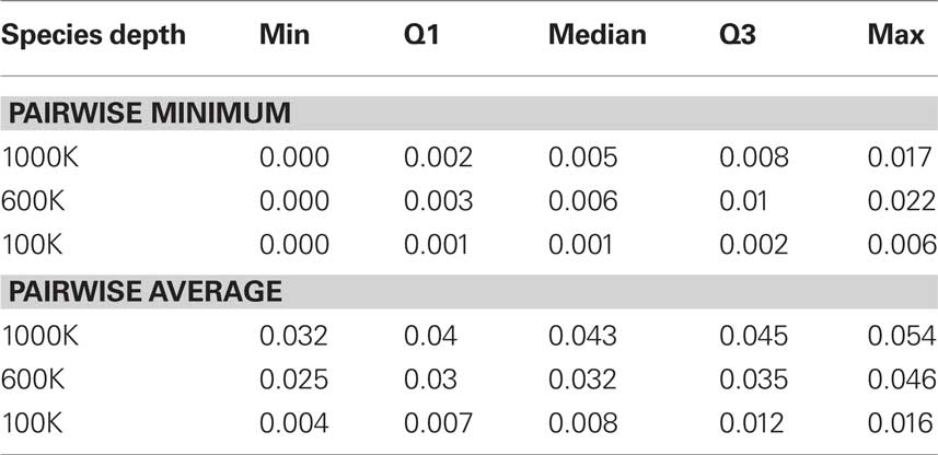
Table 1. Q1 means the first quartile and Q3 means the third quartile. By “min” we mean the smallest number and “max” means the largest number among a sample. Sequence divergences were calculated in two ways: (i) the pairwise minimum percentage of sequence divergence and (ii) the average pairwise percentage of sequence divergence.

In order to estimate posterior distributions we used the MCMC-based software MrBayes with the following parameters: (i) for the model: HKY85 + Gamma, shape parameter: 0.8, transition–transversion ratio: 3.0; and (ii) for MCMC runs: number of runs: 1, number of chains: 2, chain length: 100,000, sample frequency: 1,000, burn-in: 25%. For bootstrap sampling we sampled 100 bootstrap samples with sample size of 1,000 columns since the simulated sequences are generated with 1,000 base pairs.

We generated simulated data sets in three different ways; (i) two separate sequence data sets generated from the same gene tree, (ii) sequence data sets generated from two different gene trees under the same species tree, (iii) sequence data sets generated by two sequence data sets generated from two different gene trees whose species trees are also different. We tested 10 gene trees for each species depth (i.e., 30 different gene trees in total) generated under the same species tree. One can find the species trees we used in Figure 2. We used two sets of sequences generated under the HKY model with the same tree for each test. We have the three species depths of 1000,000, 600,000, and 100,000, with fixed population size of 100,000. Notice that we do not observe any Type I errors with our testing method, however, in within-species comparisons at species depth of 1,000,000 the p-values were high in general. Also notice that with pairs of gene trees where each pair of gene trees are generated from different species trees under the coalescence model, the p-values were less than 0.001 for all pairs of genes from 1,000,000 and 600,000 species depth. However, in the case of species depth 100,000 we see that only one pair (Species1_g0/Species2_g7) has a p-value less than 0.05 (see Table S4 in Supplementary Material).

FIGURE 1

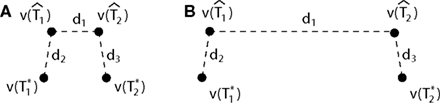
Figure 1. A diagram showing two cases of the differences of means method. is the estimator of T₁ and is the estimator of T₂. is a tree sampled from the distribution for T₁ and is a tree sampled from the distribution for T₂. In (A), the triangle inequality in Eq. 2 under the assumption of the null hypothesis does not hold, namely . In (B), the triangle inequality Eq. 2 under the assumption of the null hypothesis holds, namely .

FIGURE 2

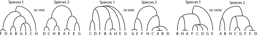
Figure 2. The three pairs of species trees used in our simulations. The dissimilarity maps normalized by between the two species trees used to generate gene trees for our simulations are 0.4333 for 1,000,000 species depth, 0.2672 for 600,000 species depth, and 0.046 for 100,000 species depth.

p-values and distance between true trees appear strongly correlated. We fitted correlations between p-values and distance between true trees as well as correlation between p-values and the difference of means for the posterior distributions given the original sequence data sets, using a function called loess (Figure 3A). The fitted lines show negative correlation between the p-values and the distance between true trees and also negative correlation between the p-values and the difference of means. Note that the fitted lines for distances between true trees and for differences of means in Figure 3A any p-values below the α-level (0.05 in our case) are within their confidence intervals. Actually they are within their confidence intervals up to the p-value equals to 0.3. This means the differences of means with posterior distributions given the original sequence data sets are good measurements for distance between true trees for our statistical tests. This is particularly important since we usually do not know the true trees with biological data sets. For complete results of our simulations see Tables S1 and S3 in Supplementary Material. We appear to have Type II errors, since the distance between the true gene trees are very close to each other (see Table S4 in Supplementary Material). Also, since the bound provided in Eq. 2 is not tight for some cases, the bound coming from Eq. 2 is conservative, i.e., it tends to give higher p-values. Thus we have some power loss in our method.

FIGURE 3

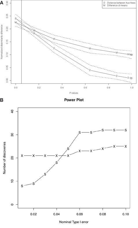
Figure 3. (A) Correlation between p-values and dissimilarity map distances, for the data sets. For each data set, the plotted “D” point represents the distance between the true trees , and the plotted “M” point represents the distance between the posterior means given the sequence data. The number of data sets is 84. For more details see the Supplementary Material. We fitted the data in R (R Development Core Team, 2004) using loess for local regression. The dotted lines are for 95% confidence intervals of the fitted lines. The vertical solid line is the p-value cutoff α = 0.05. (B) Power comparison of our method vs. the “paired SH test” described in the main text. The “X” line plots the number of discoveries for our method; the “S” line is for the SH test.

TABLE 2

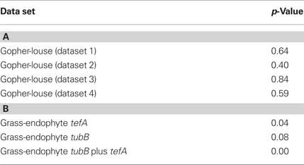
Table 2. (A) p-Values for subsets of the well-known gopher-louse data set in Hafner and Nadler (1990). All p-values are high, so no significant incongruence is found. (B) p-Values for grass-endophyte data sets from Schardl et al. (2008). After removing cases of apparent host jumps, the data comprises 20 taxa of grasses and 20 taxa of endophytes. The first two rows compare grass phylogeny to gene trees for tefA and tubB in endophytes; the last row uses the concatenation of tefA and tubB.

TABLE 3

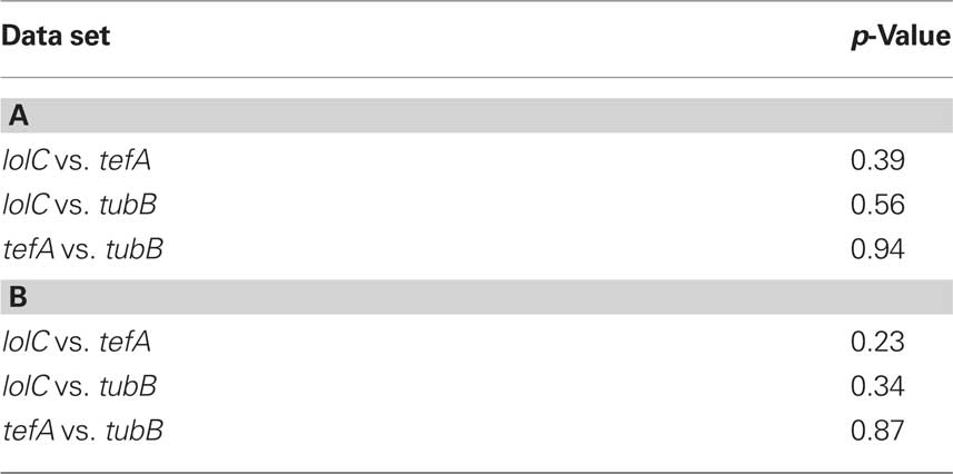
Table 3. (A) The results with our statistical method with the endophyte data sets from lolC, tubB, tefA genes. There are 17 taxa in each data set. (B) The results with our statistical method with the endophyte data sets from lolC, tubB, tefA genes after removing E2368. There are 16 taxa in each data set.

We also compared our method with two others: the statistical hypothesis testing described in Example 3 of Section 4.4.1 in Holmes (2005), and an application of the SH test (Shimodaira and Hasegawa, 1999). For the method in Holmes (2005), to compute the ML trees we used Raxml (Stamatakis, 2006), and to compute p-values we used R (Feinerer and Hornik, 2009). We used a bootstrap sample size of 1,000. In our simulations, the method in Holmes (2005) had higher power than ours, but it exhibited a 13% of Type I error, while our method committed no Type I errors (see Tables S1 and S3 in Supplementary Material for details).

For SH test we used paup* (Swofford, 1998). The bootstrap sample size was chosen to be 100 (the same as our method), and the number of random tree topologies was chosen to be 1000. Note that SH is designed to test whether a given tree T₁ is contained in the confidence region for an unknown tree T₂. In our framework, both T₁ and T₂ are unknown. Thus we applied the SH procedure twice: once to test whether the ML estimate is in the confidence region for T₂, and once to test whether is in the confidence region for T₁. If both tests reject, then we declare that the overall procedure rejects T₁ = T₂. We call this the “paired SH test.” To run the paired SH test at level α, each of the two individual SH tests is run at level α.

With these parameters, neither SH nor our method exhibited any false positives when the nominal Type I error rate was set to α ≤ 0.1. For α ≥ 0.05, SH had slightly more power, but our method was much more powerful than SH for small α. See Figure 3B for a power comparison of our method against SH; also Tables S1 and S3 in Supplementary Material contain detailed p-value information for each test.

Experiments with Real Data Sets

We tested our method with a well-known gopher-louse data set (Hafner and Nadler, 1990), see Table 2. This data set contains 17 taxa of lice and 15 taxa of gophers. In order to satisfy the requirement for an equal number of leaves for tree comparison we constructed four individual data sets reflecting all possible pairings of the two gopher species involved in the possible host jumps with their apparent parasitic louse species: (dataset 1) Thomomys talpoides–Thomomydoecus barbarae, Thomomys bottae–Thomomydoecus minor; (dataset 2) Thomomys talpoides–Geomydoecus thomomyus, Thomomys bottae–Thomomydoecus minor; (dataset 3) Thomomys talpoides–Thomomydoecus barbarae, Thomomys bottae–Geomydoecus actuosi; (dataset 4) Thomomys talpoides–Geomydoecus thomomyus, Thomomys bottae–Geomydoecus actuosi.

The posterior distributions were estimated using MrBayes with the following parameters: (i) for the model: GTR + Gamma + Invariant sites; (ii) for MCMC: number of runs: 1, number of chains: 2, chain length: 100,000, sample frequency: 1,000, burn-in: 25%; and (iii) for bootstrap sampling: 100 bootstrap samples with sample size of 379 columns which is the length of sequence alignments in the data sets.

We also tested our Method with the data sets from Schardl et al. (2008). After removing cases of apparent host jumps, the data sets contain sequences from 20 taxa of grasses and 20 taxa of endophytes. Sequences were aligned with the aid of PILEUP implemented in SEQWeb Version 1.1 with Wisconsin Package Version 10 (Genetics Computer Group, Madison, WI). PILEUP parameters were adjusted empirically; a gap penalty of 2 and a gap extension penalty of 0 resulted in reasonable alignment of intron–exon junctions and intron regions of endophyte sequences, and of intergenic spacer and intron regions of cpDNA sequences. Alignments were scrutinized and adjusted by eye, using tRNA or protein coding regions as anchor points. For phylogenetic analysis of the symbionts, sequences from tubB (encoding β-tubulin) and tefA (encoding translation elongation factor 1-α) were concatenated to create a single, contiguous sequence of approximately 1400 bp for each endophyte, of which 357 bp was exon sequence and the remainder was intron sequence. For phylogenetic analysis of the hosts, sequences for both cpDNA intergenic regions (trnT-trnL and trnL-trnF) and the trnL intron were aligned individually then concatenated to give a combined alignment of approximately 2200 bp. Analysis was also performed using the sequences from tubB and tefA separately.

The posterior distributions were estimated using MrBayes with the following parameters: (i) for the model: GTR + Gamma + Invariant sites; (ii) for MCMC: number of runs: 1, number of chains: 2, chain length: 100,000, sample frequency: 1,000, burn-in: 25%; and (iii) for bootstrap sampling: 100 bootstrap samples, number of bootstrap columns equals length of original alignment.

These results are interesting in comparison with the prior finding of significant relationship between the phylogenies of the grasses and their endophytes (Schardl et al., 2008). The previous analysis indicated a significant relationship between ages of corresponding nodes in endophyte and grass phylogenies, addressing whether divergences of grass and endophyte clades tended to occur at approximately the same time. In contrast, results of the analysis above suggest that the grass and endophyte phylogenies are significantly different (Table 2). We conclude that such a relationship of node ages does not necessarily imply similar phylogenetic histories. This is reasonable because the relationships of grasses and their endophytes is expected to be one of diffuse cospeciation at best. Individual species of endophyte may be associated with genera or tribes of grasses, but rarely with individual species. This contrasts with the gopher–gopher louse situation, where evidence suggests a much stricter coevolutionary relationship (Table 2).

We chose an additional biological data set to compare phylogenies of genes that occur together in endophyte genomes. Whereas tefA and tubB are housekeeping genes present in all isolates, lolC is a secondary metabolism gene sporadically present in endophyte isolates (Spiering et al., 2002). It has been suggested that such sporadically occurring secondary metabolism genes may be distributed in fungi largely by horizontal gene transfer (Walton, 2000). To investigate this possibility in the case of lolC, we used our approach to test whether the phylogenies of these three genes were significantly different. The most likely trees obtained by MCMC showed related but non-identical topologies (Figure 4; note placement of genes from Epichloe festucae and Epichloe brachyelytri). Our test found no significant difference between the phylogenies, although the p-values appear stochastically smaller than the p-values observed for simulated data under the null. This perhaps reflects the conservative nature of our test. Removing either Epichloe festucae or Epichloe brachyelytri altered the results only slightly (Table 3). These results indicate that lolC evolution was largely or exclusively by decent, and disfavored horizontal transfer as an explanation for the sporadic distribution of this gene.

FIGURE 4

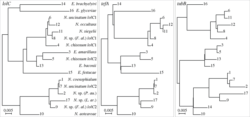
Figure 4. Trees with maximum likelihood identified by MCMC search on aligned intron sequences from the lolC, tefA, and tubB genes of Epichloe and Neotyphodium species. Some Neotyphodium species are interspecific hybrids that have multiple genomes from different ancestors. The genes from the different genomes are distinguished, for example, as lolC1 and lolC2. The same number labeling leaves on the three trees indicates genes from the same genome from the same fungal isolate.

Toolkit for Computational Experiments

To facilitate computations for our experiments, we developed a set of programs, collectively called Phylotree. Phylotree is organized as a collection of scripts for running a complete computational experiment starting from sequence alignments, then sampling phylogenetic trees and computing distances between phylogenetic trees and their distributions (see Section “Materials and Methods”). Supported distance measures include path difference, dissimilarity map distance, Robinson–Foulds distance. Available scripts allow for selecting the number of columns and the number of bootstrap samples, linking taxa in the alignments and provide flexibility for using different sampling methods (e.g., MrBayes or BEAST) and distance measures. This is free software, and will be distributed under the terms of the GNU General Public License. One can download the software at http://csurs7.csr.uky.edu/phylotree/. The login information can be obtained at http://cophylogeny.net/research.php..

Discussion

In this paper we presented a method to determine if two phylogenetic trees with given alignments are significantly incongruent. Our method computes the difference of means of posterior distributions of trees, which has the advantage of using entire tree distributions, as opposed to single tree estimators.

In this paper we used the triangle inequality (d₁ ≤ d₂ + d₃ in Figure 1) to derive a bootstrap procedure to compute p-values (we included the box plots for p-values and the ROC curve for our method, see Figures S1 and S2 in Supplementary Material). However, our bootstrap procedure appears to be very conservative, producing p-values whose null distribution is stochastically much larger than uniform U(0,1). Thus in order to increase the power we might want to consider different criteria for computing p-values. One approach may be to define to be the average of bootstraps , rather than the initial tree estimates. Another possibility is to replace the triangle inequality with a max condition [e.g., in Figure 1 use the condition d₁ ≤ max(d₂,d₃)]. We explored this in the Supplementary Material, and it seems that the max condition provides much more power, but is somewhat anti-conservative.

In this paper we used the dissimilarity map as a feature space. However, there are other common tree features which can be used to define different feature spaces. Examples of distances derived from tree features include (normalized) Robinson–Foulds distance (Robinson and Foulds, 1981); quartet distance (Estabrook et al., 1985); and the path difference metric (Steel and Penny, 1993). Of course, in all the above examples, we could choose any vector space norm, such as L_p for any p. The important point is that there are many different useful features (i.e., choices of maps into a normed space) which can be used to analyze trees, and many such as splits and quartets have already been used for quite some time. Moreover, with the kernel method presented above we can efficiently calculate distances between distributions of trees using the Robinson–Foulds and quartet distance. Thus it is interesting to use different feature spaces for our statistical method, and we leave this for future work.

Conflict of Interest Statement

The authors declare that the research was conducted in the absence of any commercial or financial relationships that could be construed as a potential conflict of interest.

Acknowledgments

David Haws, Elissaveta Arnaoudova, Jerzy W. Jaromczyk, Christopher L. Schardl, Ruriko Yoshida are supported by NIH R01 grant 5R01GM086888. Elissaveta Arnaoudova, Jerzy W. Jaromczyk, and Neil Moore developed the software Phylotree. Peter Huggins is supported by the Lane Fellowship in Computational Biology at Carnegie Mellon University. We thank anonymous referees for useful comments which improve this paper.

Supplementary Material

The Supplementary Material for this article can be found online at http://www.frontiersin.org/neuroscience/systems biology/paper/10.3389/fnins.2010.00047

References

Ane, C., Larget, B., Baum, D. A., Smith, S. D., and Rokas, A. (2007). Bayesian estimation of concordance among gene trees. Mol. Biol. Evol. 24, 412–426.

Pubmed Abstract | Pubmed Full Text | CrossRef Full Text

Buneman, P. (1971). “The recovery of trees from measures of similarity,” in Mathematics of the Archaeological and Historical Sciences, eds F. Hodson, D. Kendall, and P. Tautu (Edinburgh: Edinburgh University Press), 387–395.

Edwards, S., Liu, L., and Pearl, D. (2007). High-resolution species trees without concatenation. Proc. Natl. Acad. Sci. U.S.A. 104, 5936–5941.

Pubmed Abstract | Pubmed Full Text | CrossRef Full Text

Estabrook, G., McMorris, F., and Meaeham, C. (1985). Comparison of undirected phylogenetic trees based on subtrees of four evolutionary units. Syst. Zool. 34, 193–200.

CrossRef Full Text

Feinerer, I., and Hornik, K. (2009). wordnet: WordNet Interface. R package version 0.1-5. http://CRAN.R-project.org/package=wordnet

Felsenstein, J. (1981). Evolutionary trees from DNA sequences. J. Mol. Evol. 17, 368–376.

Pubmed Abstract | Pubmed Full Text | CrossRef Full Text

Galtier, N., Gascuel, O., and Jean-Marie, A. (2005). “An introduction to Markov models in molecular evolution,” in Statistical Methods in Molecular Evolution, ed. R. Nielsen (New York: Springer), 3–24.

Ge, S., Sang, T., Lu, B., and Hong, D. (1999). Phylogeny of rice genomes with emphasis on origins of allotetraploid species. Proc. Natl. Acad. Sci. U.S.A. 96, 14400–14405.

Pubmed Abstract | Pubmed Full Text | CrossRef Full Text

Guindon, S., and Gascuel, O. (2003). A simple, fast, and accurate algorithm to estimate large phylogenies by maximum likelihood. Syst. Biol. 52, 696–704.

Pubmed Abstract | Pubmed Full Text | CrossRef Full Text

Hafner, M. S., and Nadler, S. A. (1990). Cospeciation in host parasite assemblages: comparative analysis of rates of evolution and timing of cospeciation events. Syst. Zool. 39, 192–204.

CrossRef Full Text

Holmes, S. (2005). “Statistical approach to tests involving phylogenies,” (Chapter 4) in Mathematics of Phylogeny and Evolution, ed. O. Gascuel (New York: Oxford University Press), 91–117.

Huelsenbeck, J., and Ronquist, F. (2001). Mrbayes: Bayesian inference in phylogenetic trees. Bioinformatics 17, 754–755.

Pubmed Abstract | Pubmed Full Text | CrossRef Full Text

Huggins, P., Li, W., Haws, D., Friedrich, T., Liu, J., and Yoshida, R. (2010). Bayes estimators for phylogenetic reconstruction. Syst. Biol. (in press).

Kishino, H., and Hasegawa, M. (1989). Evaluation of the maximum likelihood estimate of the evolutionary tree topologies from DNA sequence data. J. Mol. Evol. 29, 170–179.

Pubmed Abstract | Pubmed Full Text | CrossRef Full Text

Lee, M. S. Y., and Hugall, A. F. (2003). Partitioned likelihood support and the evaluation of data set conflict. Syst. Biol. 52, 15–22.

Pubmed Abstract | Pubmed Full Text | CrossRef Full Text

Liu, L., and Pearl, D. (2007). Species trees from gene trees: reconstructing Bayesian posterior distributions of a species phylogeny using estimated gene tree distributions. Syst. Biol. 56, 504–514.

Pubmed Abstract | Pubmed Full Text | CrossRef Full Text

Liu, L., Pearl, D., Brumfield, R., and Edwards, S. (2008). Estimating species trees using multiple-allele DNA sequence data. Evolution 62, 2080–2091.

Pubmed Abstract | Pubmed Full Text | CrossRef Full Text

Maddison, W. (1997). Gene trees in species trees. Syst. Biol. 46, 523–536.

Maddison, W., and Knowles, L. (2006). Inferring phylogeny despite incomplete lineage sorting. Syst. Biol. 55, 21–30.

Pubmed Abstract | Pubmed Full Text | CrossRef Full Text

R Development Core Team. (2004). R: A Language and Environment for Statistical Computing. Vienna: R Foundation for Statistical Computing. http://www.R-project.org.

Robinson, D. F., and Foulds, L. R. (1981). Comparison of phylogenetic trees. Math. Biosci. 53, 131–147.

CrossRef Full Text

Saitou, N., and Nei, M. (1987). The neighbor joining method: a new method for reconstructing phylogenetic trees. Mol. Biol. Evol. 4, 406–425.

Pubmed Abstract | Pubmed Full Text

Schardl, C. L., Craven, K. D., Speakman, S., Lindstrom, A., Stromberg, A., and Yoshida, R. (2008). A novel test for host-symbiont codivergence indicates ancient origin of fungal endophytes in grasses. Syst. Biol. 57, 483–498.

Pubmed Abstract | Pubmed Full Text | CrossRef Full Text

Shimodaira, H., and Hasegawa, M. (1999). Multiple comparisons of log-likelihoods with applications to phylogenetic inference. Mol. Biol. Evol. 16, 1114–1116.

Spiering, M., Wilkinson, H., Blankenship, J., and Schardl, C. (2002). Expressed sequence tags and genes associated with loline alkaloid expression by the fungal endophyte neotyphodium uncinatum. Fungal Genet. Biol. 36, 242–254.

Pubmed Abstract | Pubmed Full Text | CrossRef Full Text

Stamatakis, A. (2006). RAxML-VI-HPC: maximum likelihood-based phylogenetic analyses with thousands of taxa and mixed models. Bioinformatics 22, 2688–2690.

Pubmed Abstract | Pubmed Full Text | CrossRef Full Text

Steel, M., and Penny, D. (1993). Distributions of tree comparison metrics-some new results. Syst. Biol. 42, 126–141.

Swofford, D. L. (1998). PAUP*. Phylogenetic Analysis Using Parsimony (* and Other Methods). Sunderland, MA: Sinauer Associates.

Vilaa, M., Vidal-Romani, J. R., and Björklund, M. (2005). The importance of time scale and multiple refugia: incipient speciation and admixture of lineages in the butterfly Erebia triaria (Nymphalidae). Mol. Phylogenet. Evol. 36, 249–260.

Pubmed Abstract | Pubmed Full Text | CrossRef Full Text

Voigt, K., Cicelnik, E., and O’Donnel, K. (1999). Phylogeny and PCR identification of clinically important zygomycetes based on nuclear ribosomal-DNA sequence data. J. Clin. Microbiol. 37, 3957–3964.

Pubmed Abstract | Pubmed Full Text

Walton, J. (2000). Horizontal gene transfer and the evolution of secondary metabolite gene clusters in fungi: an hypothesis. Fungal Genet. Biol. 30, 167–171.

Pubmed Abstract | Pubmed Full Text | CrossRef Full Text

Yang, Z., and Rannala, B. (1997). Bayesian phylogenetic inference using DNA sequences: a Markov chain Monte Carlo method. Mol. Biol. Evol. 14, 717–724.

Pubmed Abstract | Pubmed Full Text