Watersheds in disordered media

1. Introduction

Although both start in the mountains of Switzerland, the Rhine and Rhone rivers diverge while flowing toward different seas. While the Rhine empties into the North Sea, the Rhone drains into the Mediterranean. Similarly, all over the world one finds rivers with close sources but distant mouths. For example, the Colorado and the Rio Grande even open toward different oceans. When looking at a landscape, how to identify the regions draining toward one side or the other? When rain falls or snow melts on a landscape, the dynamics of the surface water is determined by the topography of the landscape. Water flows downhill and overpasses small mounds by forming lakes which eventually overspill. A drainage basin is then defined as the region where water flows toward the same outlet. Its shape and extension strongly depend on the topography. The line separating two adjacent basins is the watershed line, which typically wanders along the mountain crests [1].

Since watersheds provide information about the dynamics of surface water, they play a fundamental role in water management [2–4], landslides [5–8], and flood prevention [8–10]. Watersheds are also of relevance in the political context they have been used to demarcate borders between countries such as the one between Argentina and Chile [11]. Thus, the understanding of their statistical properties and resilience to changes in the topography of the landscape are two important questions that we will review here. In general, for every landscape, several outlets can be defined, each one with a corresponding drainage basin. Sets of small drainage basins eventually drain toward the same outlet forming a even larger basin. Such hierarchy results in a larger number of watersheds. However, without loss of generality, the study of watershed lines can be simplified by splitting the landscape into only two large basins, each one draining toward opposite boundaries. Figure 1 shows how this watershed can be identified by flooding the landscape from the valleys (see Supplemental video). Two sinks are initially defined (the lower-left and upper-right boundaries in the example). While flooding the landscape, each time two lakes (A and B) draining toward opposite sinks are about to connect, one imposes a physical barrier between the two. In the end, the watershed line is the line formed by the barriers that separate these two lakes.

FIGURE 1

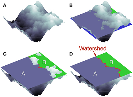
Figure 1. Watershed dividing a landscape into two parts. The landscape (A) is flooded from the valleys such that all regions lower than a certain height are covered with water (B). As the water level rises, lakes merge under the constraint that no lake can connect two predefined opposite boundaries of the landscape (C). In this example, we have taken the lower-left and the upper-right boundaries. Thus, a watershed line emerges separating the two final lakes (D). These lakes (A and B) are the drainage basins of this landscape.

The concept of watersheds is also of interest in other fields like, e.g., in medical image processing [12]. There, computed tomography scans need to be segmented to identify different tissues. The pictures are discretized into pixels and a number is assigned to each one of them according to the intensity. The segmentation procedure consists in clustering neighboring pixels following the order of increasing intensity gradient, splitting the image into different parts (tissues). The equivalent to the watershed line corresponds to the line separating two different tissues [13, 14].

It was recently shown that watersheds can be described in the context of percolation theory in terms of bridges and cutting bond models [15], with numerical evidence that they are Schramm-Loewer Evolution (SLE) curves in the continuum limit [16]. This association explains why watersheds on uncorrelated landscapes as well as other statistical physics models, such as, optimal path cracks [17–19], fuse networks [20], and loopless percolation [15], belong to the same universality class of optimal paths in strongly disordered media.

2. The Landscape

The motion of surface water is defined by the topology of the landscape, usually characterized by the spatial distribution of heights. Although this distribution is a continuous function for real landscapes, it is typically coarse-grained and represented as a digital elevation map (DEM) of regular cells (e.g., a square lattice of sites or bonds) to which average heights can be associated. This process is exemplarily shown in Figures 2A–C. In fact, modern procedures of analyzing real landscapes numerically process Grayscale Digital Images where the gray intensity of each pixel is transformed into a height, resulting in a DEM. As such, discretized maps have been useful to delimit spatial boundaries in a wide range of problems, from tracing watersheds and river networks in landscapes [21–25] to the identification of cancerous cells in human tissues [13, 26], and the study of spatial competition in multispecies ecosystems [27, 28].

FIGURE 2

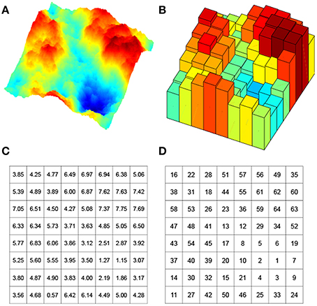
Figure 2. The process of generating a ranked surface. The landscape in (A) is coarse-grained to the low-resolution system of 8 × 8 cells shown in (B), and then represented as a discretized map of local heights, as depicted in (C). By ranking these heights in crescent order, one obtains the ranked surface in (D). In fact, the landscape shown in (A) is a high resolution synthetic map obtained from a fractional Brownian motion simulation based on the Fourier filtering method (see Section 7).

To study watersheds theoretically one can generate artificial landscapes. Starting with a regular lattice, a numerical value is randomly assigned to each element, corresponding to its average height. If these values are spatially correlated, a correlated artificial landscape is obtained. Otherwise, the landscape is called an uncorrelated artificial landscape. Natural landscapes are characterized by long-range correlations [29]. In Section 7 we will review how to generate correlated artificial landscapes and their main properties.

The DEM can be further simplified by mapping them onto ranked surfaces, where every element (site or bond) has a unique rank associated with its corresponding value [15]. A ranked surface can be defined in the following way. Given a two-dimensional discretized map of size L × L, one generates a list containing the heights of its elements (sites or bonds) in crescent order, and then replaces the numerical values in the original map by their corresponding (integer) ranks. As depicted in Figure 2D, the result is a ranked surface.

3. How to Determine the Watershed

Traditional cartographic methods for basin delineation have relied on manual estimation from iso-elevation lines. Instead, modern procedures are now based upon automatic processing of images as the ones obtained from satellites [30, 31]. These images are typically coarse-grained into discretized maps with each cell i having a height h_i as explained in Section 2. A recently proposed algorithm to identify watersheds that became rather popular consists in the flooding procedure described in Figure 3 [31], considering two sinks such as, for example, two opposite boundaries. Cells in the discretized map are ranked according to their height, which leads to a ranked surface, and are sequentially occupied, following the rank, from the lowest to the highest. Neighboring occupied cells are then connected and considered part of the same drainage basin, except when during this process their connection would promote the agglomeration of the two basins draining toward different sinks. In this case, their connection is avoided, since they should belong to different basins. The edge between them is part of the watershed and, at the end, the set of such edges forms one single watershed line that splits the landscape into two drainage basins (see Figure 3).

FIGURE 3

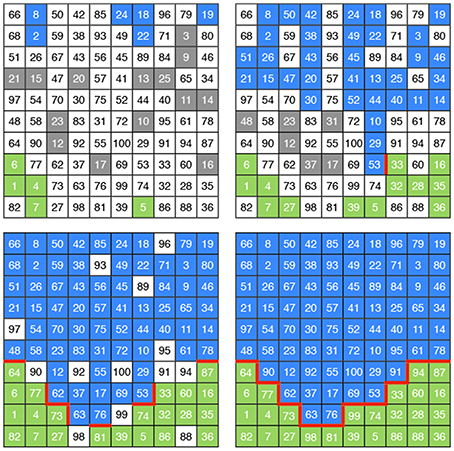
Figure 3. Flooding algorithm to determine the watershed. Two sinks are considered: the top row and the bottom one. Cells in the discretized map are occupied following the rank, from the lowest to the highest. Neighboring occupied cells are considered connected and part of the same basin (gray cells). The basins connected to the top row (blue) correspond to the ones draining toward the top sink. Similarly, the ones connected to the bottom row (green) drain toward the bottom sink (upper-left panel). If two neighbors of the next cell in the rank belong to basins of different sinks, the edges in contact with the cells are marked as elements of the watershed (red-thick edges). The process proceeds iteratively until all cells are flooded (bottom panels). At the end (bottom-right panel), the watershed splits the discretized map into two basins (blue and green).

The flooding procedure implies visiting every cell in the discretized map. Fehr and co-workers [32] have devised a more efficient identification algorithm where only a fractal subset needs to be visited. The algorithm is based on Invasion Percolation (IP) [33] and consists in the following procedure. One initially defines two sinks (for example, the bottom and top rows of the discretized map) and considers that the (non-invaded) cell with the lowest height on the perimeter of the (already) invaded region is the next cell to be invaded. If when starting from one cell a sink is invaded, the initial cell and the entire invaded region is considered to belong to the catchment basin of that sink. Consider that the invasion is initially started from the cell in the bottom-right corner. Since this cell is part of the basin of the bottom sink, the invaded region has only one cell. One proceeds with a new invasion from the next cell upwards (cell 35 in Figure 4) and a new invasion cluster is grown until a sink is reached. Sequentially, all other cells are considered in the same way. The watershed is then identified as the line splitting the landscape into two catchment basins. The efficiency is significantly improved if, once the first cell-edge belonging to the watershed has been identified, the exploration continues from the cells in the neighborhood of this edge (see Figure 4). Thus, instead of visiting all cells, only a subset of N_exp cells needs to be explored. For uncorrelated random landscapes, the size of this subset scales with the linear size of the DEM L as N_exp ~ L^D, with D = 1.8 ± 0.1 [32].

FIGURE 4

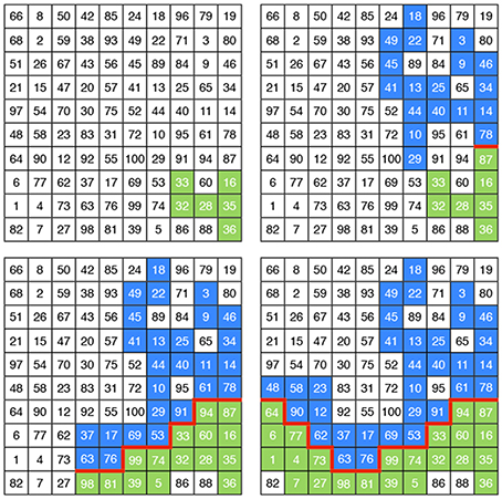
Figure 4. Algorithm based on Invasion Percolation. As in Figure 3, two sinks are considered: the top and the bottom rows. One starts from the bottom-right corner (cell 36). Since this site is in the bottom row, it is already part of the bottom sink (green). Proceeding upwards, following the most right column, the next unexplored cell is considered (cell 35). The basin to which this cell belongs grows by adding the smallest-height cell on its perimeter, until one sink is reached (cells 16, 28, 32, and 33 in the upper-left panel, reaching 36). Proceeding further to the top, the cell 87 is added to the (green) basin (connecting to 16). When the cell 78 is considered and the corresponding basin grown, a new (blue) basin is found draining toward the upper sink (upper-right panel). The cell-edge between cell 87 and 78 is considered part of the watershed (red-thick edge). Proceeding by iteratively identifying the basin of the cells in the neighborhood of the watershed edges, the full watershed is identified (bottom panels). Since the same initial ranked surface is considered, the final watershed is equal to the one obtained in Figure 3.

4. Fractal Dimension

Breyer and Snow [35] have studied 12 basins in the United States and concluded that their watershed lines are self-similar objects [36, 37]. A self-similar structure is characterized by its fractal dimension d_f, which is defined here through the scaling of the number M of edges belonging to the watershed with the linear size L of the discretized map,

$\begin{array}{cc}M~L^{d_f}.& \left(1\right)\end{array}$

They obtained fractal dimensions in the range 1.05−1.12. Fehr and co-workers [32], with the method described in Section 3 confirmed this self-similar behavior over more than three orders of magnitude and measured the fractal dimension for watersheds in several real landscapes, as summarized in Table 1.

TABLE 1

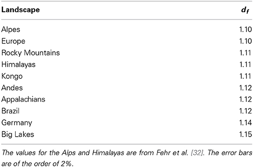
Table 1. Fractal dimension of watersheds for natural landscapes obtained from satellite imagery [30] in [34].

For uncorrelated artificial landscapes the watershed fractal dimension has been estimated to be d_f = 1.2168 ± 0.0005 [32, 38, 39]. This value has drawn considerable attention since it was also found in several other physical models such as optimal paths in strong disorder and optimal path cracks [17–19, 40, 41], bridge percolation [15, 38, 42], and the surface of explosive percolation clusters [43, 44]. The conjecture that all these models might belong to the same universality class has opened a broad range of possible implications and applications of the properties of watersheds. As discussed in Schrenk et al. [15], the relation between most of such models can be established when they are described within the framework of ranked surfaces (see also Section 2).

5. Watersheds in Three and Higher Dimensions

Up to now, we have focused on the watershed line that divides the landscape into drainage basins for water on the surface. However, in reality, water also penetrates the soil and flows underground. Thus, the concept of watersheds and ranked surfaces can be extended to three dimensions. The soil can be described as a porous medium consisting of a network of pores connected through channels. When a fluid penetrates through this medium, a threshold pressure p_k can be defined for each channel k such that the channel can only be invaded when p ≥ p_k, where p is the fluid pressure. In general, a channel k is closed when p_k > p, and open otherwise. This system can be mapped into a three dimensional ranked volume, where the lattice elements are the channels and the rank is defined by the increasing order of the threshold pressure. The sequence in the rank corresponds to the order of channel openings when the fluid pressure is quasistatically raised from zero. Analogously to the ranked surfaces, one can split the space in two regions, draining toward opposite boundaries.

The watershed in three dimensions is a surface of fractal dimension d_f = 2.487 ± 0.003 [39]. An example for a simple-cubic ranked volume is shown in Figure 5. In general, for lattices of size L^d, where d is the spatial dimension, the watershed blocks connectivity from one side to the other. Thus, the watershed fractal dimension must follow d − 1 ≤ d_f ≤ d, i.e., with increasing dimension d_f also increases [15].

FIGURE 5

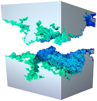
Figure 5. Watershed in three dimensions. Example of a watershed for an uncorrelated three-dimensional space, namely, a simple-cubic lattice of 128³ sites. To obtain the watershed, sites are sequentially occupied under the constraint that groups of connected sites in contact with the top boundary cannot merge with the ones connected to the bottom boundary. In three dimensions, the fractal dimension is d_f = 2.487 ± 0.003 [39].

6. Impact of Perturbation on Watersheds

The stability of watersheds is also a subject of interest. For example, changes in the watershed might affect the sediment supply of rivers [45]. Also, the understanding of the temporal evolution of drainage networks provides valuable insight into the biodiversity between basins [46]. Geographers and geomorphologists have found that the evolution of watersheds is typically driven by local changes of the landscape [47]. These events can be triggered by various mechanisms like erosion [46, 48, 49], natural damming [8], tectonic motion [50–52], as well as volcanic activity [53]. Although rare, these local events can have a huge impact on the hydrological system [47–49, 54]. For example, it was shown that a local height change of less than two meters at a location close to the Kashabowie Provincial Park, some kilometers North of the US-Canadian border, can trigger a displacement in the watershed such that the area enclosed by the original and the new watersheds is about 3730 km² [55].

The stability of watersheds is also relevant in the political context. For example, Chile and Argentina share a common border with more than 5000 kilometers, which was the source of a long dispute between these countries [11]. A treaty established this border as being the watershed between the Atlantic and Pacific Oceans for several segments. In 1902, the Argentinian Francisco Moreno contributed significantly to elucidate the technical basis for dispute. He proved that during the quarternary glaciations, the watershed line changed. In particular, several Patagonian lakes currently draining to the Pacific Ocean were in fact originally part of the Atlantic Ocean basin. Consequently, he argued, instead of belonging to Chile they should be awarded to Argentina.

Douglas and Schmeeckle [45] have performed fifteen table top experiments to study the mechanisms of drainage rearrangements. In spite of being diverse, the mechanisms triggering the evolution of watersheds are all modifications of the topography [8, 46, 50]. In that perspective, the effect of such events can be investigated by applying small local perturbations to natural and artificial landscapes and analyzing the changes in the watershed [34, 55]. Specifically, one starts with a discretized landscape and computes the original watershed. A local event is then induced by changing the height of a site k, h_k → h_k + Δ, where Δ is the perturbation strength, and the new watershed is identified. The impact of perturbations on watersheds in two and three dimensions will be discussed in the following.

6.1. Impact of Perturbations in Two Dimensions

Fehr and co-workers [55] have normalized the perturbation strength by the height difference between the highest and lowest height of the landscape. For each landscape, they have sequentially perturbed every site of the corresponding discretized map, such that each perturbed landscape differs from the original only in one single site. The effect of those perturbations affecting the watershed has been quantified by the properties of the region enclosed by the original and the new watersheds. For that region, they have measured its area, corresponding to the number of sites, N_s, in the discretized map and the distance R between its original and new outlets, defined as the points where water escapes from this region. Note that, there are only two outlets involved in this procedure: one related to the original landscape and the other to the new one. Since Δ is strictly positive, the outlet in the new landscape corresponds always to the perturbed site k.

Scale-free behavior has been found for the distribution P(N_s) of the number of enclosed sites N_s, the probability distribution P(R) of the distance R between outlets, and the dependence of the average 〈 N_s〉 on R [34, 55]. Specifically,

$\begin{array}{cc}P(N_s)~N_s^{-\beta },& \left(2\text{a}\right)\end{array}$

$\begin{array}{cc}P(R)~R^{-\rho },& \left(2\text{b}\right)\end{array}$

$\begin{array}{cc}\langle N_s\rangle ~R^{\sigma },& \left(2\text{c}\right)\end{array}$

where the measured exponents are summarized in Table 2. The power-law decay (2b) and the relation (2c) imply that a localized perturbation can have a large impact on the shape of the watershed even at very large distances, hence having a non-local effect. Additionally, the analysis of the fraction of perturbed sites affecting the watershed revealed a power-law scaling with the strength Δ. This finding supports the conclusion that changes in the watershed can be even triggered by anthropological small perturbations [55].

TABLE 2

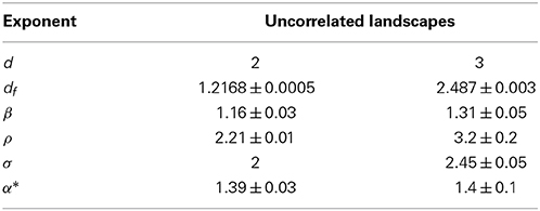
Table 2. Exponents for the impact of perturbations on watersheds, calculated for uncorrelated artificial landscapes in two and three dimensions, from [34, 39, 55, 56].

For the region enclosed by the original and the new watersheds, an invasion percolation (IP) cluster can be obtained by imposing a pressure drop between the outlet in the new watershed and the one in the original one, always invading along the steepest descent of the entire cluster perimeter. The size distribution P(M_IP|R) of these clusters, for each fixed distance R between outlets, has been shown to scale as,

$\begin{array}{cc}P(M_{\text{IP}}|R)~M_{IP}^{-(1+{\alpha }^{*})},& \left(3\right)\end{array}$

where α* ≈ 1.39. This exponent corresponds to the one found for the size distribution of point-to-point IP-clusters [57]. In that process, invasion clusters are obtained in a random medium by invading from one point to another at a certain distance. By contrast, in the watershed case the invasion is always started from the outlet on the new watershed. This difference between starting at any point or in the outlet justifies the additional factor of unity in the scaling [Equation (3)], since the probabilities need to be rescaled by the size of the IP-cluster [55].

6.2. Impact of Perturbations in Three Dimensions

The impact of perturbations on watersheds has been also analyzed in three dimensions [34]. Similar to 2D, a perturbation is induced by changing the value of a site k, h_k → h_k + Δ, where Δ is the perturbation strength. The number of sites N_s enclosed by the original and new watersheds corresponds to a volume. Power-law scaling in terms of Equations (2a)–(2c) has also been observed with the exponents summarized in Table 2. The value of α* is similar to the one found in two dimensions. According to Lee [58], the size distribution of the point-to-point IP-cluster is independent on the dimensionality of the system. Therefore, the numerical agreement between α* for different spatial dimensions supports the relation with invasion percolation.

7. Watersheds on Long-range Correlated Landscapes

Results discussed heretofore were obtained on random uncorrelated landscapes. However real landscapes are characterized by spatial long-range correlated height distributions. Numerically, such distributions can be generated from fractional Brownian motion (fBm) [36, 59], using the Fourier filtering method [19, 55, 60–70]. This method allows to control the nature and the strength of correlations, which are characterized by the Hurst exponent H. The uncorrelated distribution of heights is solely obtained for H = − d/2, i.e., H = −1 and H = −3/2 in two and three dimensions, respectively. A detailed description of this method can be found, e.g., in Oliveira et al. [19], Peitgen and Saupe[59].

Fehr et al. [34, 55] used fractional Brownian motion (fBm) on a square lattice [71] to incorporate long-range correlations controlled by the Hurst exponent H. They calculated how the fractal dimension decreases with the Hurst exponent and found good quantitative agreement with the exponents obtained for natural landscapes, typically with 0.3 < H < 0.5, which is the known range of Hurst exponents for real landscapes on length scales larger than 1 km (see Pastor-Satorras and Rothman 29 and references therein). They also obtained α, β and ρ for several values of H, observing that both β and ρ increase with H, finding also good quantitative agreement. Thus, their model provides a complete quantitative description of the effects observed on natural landscapes.

8. Final Remarks

Here we solely discussed cases with one watershed, but the same theoretical framework can be straightforwardly extended to tackle other space partition problems. For example, the identification of the entire set of watersheds of a landscape with multiple outlets helps identifying the catchment areas contributing to each river or reservoir [72]. A systematic study of disordered media with multiple outlets is still missing. Examples of open questions are: How does the distribution of catchment basins or the number of triplets (points where two watersheds meet) depend on the number of outlets? And, how does the statistics of perturbations change in the presence of triplets? The division of a volume into several parts is also a problem of practical interest in the extraction of resources from porous soils [73]. Studies of such systems have mainly considered uncorrelated disordered media. The role of long-range correlation there is still an open problem.

Conflict of Interest Statement

The authors declare that the research was conducted in the absence of any commercial or financial relationships that could be construed as a potential conflict of interest.

Acknowledgments

We acknowledge financial support from the European Research Council (ERC) Advanced Grant 319968-FlowCCS, the Brazilian Agencies CNPq, CAPES, FUNCAP and FINEP, the FUNCAP/CNPq Pronex grant, the National Institute of Science and Technology for Complex Systems in Brazil, the Portuguese Foundation for Science and Technology (FCT) under contracts no. IF/00255/2013, PEst-OE/FIS/UI0618/2014, and EXCL/FIS-NAN/0083/2012, and the Swiss National Science Foundation under Grant No. P2EZP2-152188.

Supplementary Material

The Supplementary Material for this article can be found online at: https://www.frontiersin.org/Journal/10.3389/fphy.2015.00005/abstract

References

1. Gregory KJ, Walling DE. Drainage Basin form and Process: A Geomorphological Approach. London: Edward Arnold (1973).

Google Scholar

2. Vörösmarty CJ, Federer CA, Schloss AL. Potential evaporation functions compared on US watersheds: Possible implications for global-scale water balance and terrestrial ecosystem modeling. J Hydrol. (1998) 207:147. doi: 10.1016/S0022-1694(98)00109-7

CrossRef Full Text | Google Scholar

3. Kwarteng AY, Viswanathan, MN, Al-Senafy MN, Rashid T. Formation of fresh ground-water lenses in northern Kuwait. J Arid Environ. (2000) 46:137–55. doi: 10.1006/jare.2000.0666

CrossRef Full Text | Google Scholar

4. Sarangi A, Bhattacharya AK. Comparison of artificial neural network and regression models for sediment loss prediction from Banha watershed in India. Agric Water Manage. (2005) 78:195–208. doi: 10.1016/j.agwat.2005.02.001

CrossRef Full Text | Google Scholar

5. Dhakal AS, Sidle RC. Distributed simulations of landslides for different rainfall conditions. Hydrol Process. (2004) 18:757–76. doi: 10.1002/hyp.1365

CrossRef Full Text | Google Scholar

6. Pradhan B, Singh RP, Buchroithner MF. Estimation of stress and its use in evaluation of landslide prone regions using remote sensing data. Adv Space Res. (2006) 37:698–709. doi: 10.1016/j.asr.2005.03.137

CrossRef Full Text | Google Scholar

7. Lazzari M, Geraldi E, Lapenna V, Loperte A. Natural hazards vs. human impact: an integrated methodological approach in geomorphological risk assessment on the Tursi historical site, Southern Italy. Landslides (2006) 3:275–87. doi: 10.1007/s10346-006-0055-y

CrossRef Full Text | Google Scholar

8. Lee KT, Lin YT. Flow analysis of landslide dammed lake watersheds: a case study. J Am Water Resour Assoc. (2006) 42:1615–28. doi: 10.1111/j.1752-1688.2006.tb06024.x

CrossRef Full Text | Google Scholar

9. Burlando P, Mancini M, Rosso R. FLORA: a distributed flood risk analyser. IFIP Trans B (1994) 16:91.

Google Scholar

10. Yang D, Zhao Y, Armstrong R, Robinson D, Brodzik MJ. Streamflow response to seasonal snow cover mass changes over large Siberian watersheds. J Geophys Res. (2007) 112:F02S22. doi: 10.1029/2006JF000518

CrossRef Full Text | Google Scholar

11. United Nations. The Cordillera of the Andes Boundary Case (Argentina, Chile), 20 November 1902; 2006. Available online at: http://legal.un.org/riaa/cases/vol_IX/29-49.pdf

12. Dixon JK. Pattern recognition with partly missing data. IEEE T Syst Man Cyb. (1979) 9:617. doi: 10.1109/TSMC.1979.4310090

CrossRef Full Text | Google Scholar

13. Yan J, Zhao B, Wang L, Zelenetz A, Schwartz LH. Marker-controlled watershed for lymphoma segmentation in sequential CT images. Med Phys. (2006) 33:2452. doi: 10.1118/1.2207133

Pubmed Abstract | Pubmed Full Text | CrossRef Full Text | Google Scholar

14. Patil CM, Patilkulkarani S. An approach of iris feature extraction for personal identification. IEEE Proc ARTCom. (2009) 2009:796–99. doi: 10.1109/ARTCom.2009.14

CrossRef Full Text | Google Scholar

15. Schrenk KJ, Araújo NAM, Andrade Jr JS, Herrmann HJ. Fracturing ranked surfaces. Sci Rep. (2012) 2:348. doi: 10.1038/srep00348

Pubmed Abstract | Pubmed Full Text | CrossRef Full Text | Google Scholar

16. Daryaei E, Araújo NAM, Schrenk KJ, Rouhani S, Herrmann HJ. Watersheds are schramm-loewner evolution curves. Phys Rev Lett. (2012) 109:218701. doi: 10.1103/PhysRevLett.109.218701

Pubmed Abstract | Pubmed Full Text | CrossRef Full Text | Google Scholar

17. Andrade Jr JS, Oliveira EA, Moreira AA, Herrmann HJ. Fracturing the optimal paths. Phys Rev Lett. (2009) 103:225503. doi: 10.1103/PhysRevLett.103.225503

Pubmed Abstract | Pubmed Full Text | CrossRef Full Text | Google Scholar

18. Andrade Jr JS, Reis SDS, Oliveira EA, Fehr E, Herrmann HJ. Ubiquitous fractal dimension of optimal paths. Comput Sci Eng. (2011) 13:74. doi: 10.1109/MCSE.2011.16

CrossRef Full Text | Google Scholar

19. Oliveira EA, Schrenk KJ, Araújo NAM, Herrmann HJ, Andrade Jr JS. Optimal-path cracks in correlated and uncorrelated lattices. Phys Rev E. (2011) 83:046113. doi: 10.1103/PhysRevE.83.046113

Pubmed Abstract | Pubmed Full Text | CrossRef Full Text | Google Scholar

20. Moreira AA, Oliveira CLN, Hansen A, Araújo NAM, Herrmann HJ, Andrade Jr JS. Fracturing highly disordered materials. Phys Rev Lett. (2012) 109:255701. doi: 10.1103/PhysRevLett.109.255701

Pubmed Abstract | Pubmed Full Text | CrossRef Full Text | Google Scholar

21. Stark CP. An invasion percolation model of drainage network evolution. Nature (1991) 352:423. doi: 10.1038/352423a0

CrossRef Full Text | Google Scholar

22. Maritan A, Colaiori F, Flammini A, Cieplak M, Banavar JR. Universality classes of optimal channel networks. Science (1996) 272:984. doi: 10.1126/science.272.5264.984

Pubmed Abstract | Pubmed Full Text | CrossRef Full Text

23. Manna SS, Subramanian B. Quasirandom spanning tree model for the early river network. Phys Rev Lett. (1996) 76:3460. doi: 10.1103/PhysRevLett.76.3460

Pubmed Abstract | Pubmed Full Text | CrossRef Full Text | Google Scholar

24. Knecht CL, Trump W, ben-Avraham D, Ziff RM. Retention capacity of random surfaces. Phys Rev Lett. (2012) 108:045703. doi: 10.1103/PhysRevLett.108.045703

Pubmed Abstract | Pubmed Full Text | CrossRef Full Text | Google Scholar

25. Baek SK, Kim BJ. Critical condition of the water-retention model. Phys Rev E. (2012) 85:032103. doi: 10.1103/PhysRevE.85.032103

Pubmed Abstract | Pubmed Full Text | CrossRef Full Text | Google Scholar

26. Ikedo Y, Fukuoka D, Hara T, Fujita H, Takada E, Endo T, et al. Development of a fully automatic scheme for detection of masses in whole breast ultrasound images. Med Phys. (2007) 34:4378. doi: 10.1118/1.2795825

Pubmed Abstract | Pubmed Full Text | CrossRef Full Text

27. Kerr B, Neuhauser C, Bohannan BJM, Dean AM. Local migration promotes competitive restraint in a host-pathogen “tragedy of the commons.” Nature (2006) 442:75. doi: 10.1038/nature04864

Pubmed Abstract | Pubmed Full Text | CrossRef Full Text | Google Scholar

28. Mathiesen J, Mitarai N, Sneppen K, Trusina A. Ecosystems with mutually exclusive interactions self-organize to a state of high diversity. Phys Rev Lett. (2011) 107:188101. doi: 10.1103/PhysRevLett.107.188101

Pubmed Abstract | Pubmed Full Text | CrossRef Full Text | Google Scholar

29. Pastor-Satorras R, Rothman DH. Stochastic equation for the erosion of inclined topography. Phys Rev Lett. (1998) 80:4349. doi: 10.1103/PhysRevLett.80.4349

CrossRef Full Text | Google Scholar

30. Farr TG, Rosen PA, Caro E, Crippen R, Duren R, Hensley S, et al. The shuttle radar topography mission. Rev Geophys. (2007) 45:RG2004. doi: 10.1029/2005RG000183

CrossRef Full Text

31. Vincent L, Soille P. Watersheds in digital spaces: An efficient algorithm based on immersion simulations. IEEE T Pattern Anal. (1991) 13:583. doi: 10.1109/34.87344

CrossRef Full Text | Google Scholar

32. Fehr E, Andrade Jr JS, da Cunha SD, da Silva LR, Herrmann HJ, Kadau D, et al. New efficient methods for calculating watersheds. J Stat Mech. (2009) 2009:P09007. doi: 10.1088/1742-5468/2009/09/P09007

CrossRef Full Text

33. Wilkinson D, Willemsen JF. Invasion percolation: a new form of percolation theory. J Phys A. (1983) 16:3365. doi: 10.1088/0305-4470/16/14/028

CrossRef Full Text | Google Scholar

34. Fehr E, Kadau D, Araújo NAM, Andrade Jr JS, Herrmann HJ. Scaling relations for watersheds. Phys Rev E. (2011) 84:036116. doi: 10.1103/PhysRevE.84.036116

Pubmed Abstract | Pubmed Full Text | CrossRef Full Text | Google Scholar

35. Breyer SP, Snow RS. Drainage basin perimeters: a fractal significance. Geomorphology (1992) 5:143. doi: 10.1016/0169-555X(92)90062-S

CrossRef Full Text | Google Scholar

36. Mandelbrot B. How long is the coast of Britain? Statistical self-similarity and fractional dimension. Science (1967) 156:636. doi: 10.1126/science.156.3775.636

Pubmed Abstract | Pubmed Full Text | CrossRef Full Text | Google Scholar

37. Mandelbrot BB. The Fractal Geometry of Nature. New York, NY: Freeman (1983).

38. Cieplak M, Maritan A, Banavar JR. Optimal paths and domain walls in the strong disorder limit. Phys Rev Lett. (1994) 72:2320. doi: 10.1103/PhysRevLett.72.2320

Pubmed Abstract | Pubmed Full Text | CrossRef Full Text | Google Scholar

39. Fehr E, Schrenk KJ, Araújo NAM, Kadau D, Grassberger P, Andrade Jr JS, et al. Corrections to scaling for watersheds, optimal path cracks, and bridge lines. Phys Rev E. (2012) 86:011117. doi: 10.1103/PhysRevE.86.011117

Pubmed Abstract | Pubmed Full Text | CrossRef Full Text | Google Scholar

40. Porto M, Havlin S, Schwarzer S, Bunde A. Optimal path in strong disorder and shortest path in invasion percolation with trapping. Phys Rev Lett. (1997) 79:4060. doi: 10.1103/PhysRevLett.79.4060

CrossRef Full Text | Google Scholar

41. Buldyrev SV, Havlin S, López E, Stanley HE. Universality of the optimal path in the strong disorder limit. Phys Rev E. (2004) 70:035102(R). doi: 10.1103/PhysRevE.70.035102

Pubmed Abstract | Pubmed Full Text | CrossRef Full Text | Google Scholar

42. Cieplak M, Maritan A, Banavar JR. Invasion percolation and Eden growth: Geometry and universality. Phys Rev Lett. (1996) 76:3754. doi: 10.1103/PhysRevLett.76.3754

Pubmed Abstract | Pubmed Full Text | CrossRef Full Text | Google Scholar

43. Araújo NAM, Herrmann HJ. Explosive percolation via control of the largest cluster. Phys Rev Lett. (2010) 105:035701. doi: 10.1103/PhysRevLett.105.035701

Pubmed Abstract | Pubmed Full Text | CrossRef Full Text | Google Scholar

44. Schrenk KJ, Araújo NAM, Herrmann HJ. Gaussian model of explosive percolation in three and higher dimensions. Phys Rev E. (2011) 84:041136. doi: 10.1103/PhysRevE.84.041136

Pubmed Abstract | Pubmed Full Text | CrossRef Full Text | Google Scholar

45. Douglass J, Schmeeckle M. Analogue modeling of transverse drainage mechanisms. Geomorphology (2007) 84:22. doi: 10.1016/j.geomorph.2006.06.004

CrossRef Full Text | Google Scholar

46. Bishop P. Drainage rearrangement by river capture, beheading and diversion. Prog Phys Geog. (1995) 19:449. doi: 10.1177/030913339501900402

CrossRef Full Text | Google Scholar

47. Burridge CP, Craw D, Waters JM. An empirical test of freshwater vicariance via river capture. Mol Ecol. (2007) 16:1883. doi: 10.1111/j.1365-294X.2006.03196.x

Pubmed Abstract | Pubmed Full Text | CrossRef Full Text | Google Scholar

48. Garcia-Castellanos D, Estrada F, Jiménez-Munt I, Gorini C, Fernàndez M, Vergés J, et al. Catastrophic flood of the Mediterranean after the Messinian salinity crisis. Nature (2009) 462:778. doi: 10.1038/nature08555

Pubmed Abstract | Pubmed Full Text | CrossRef Full Text | Google Scholar

49. Linkevičiene R. Impact of river capture on hydrography and water resources: case study of Ūla and Katra catchments, south Lithuania. Holocene (2009) 19:1233. doi: 10.1177/0959683609345081

CrossRef Full Text | Google Scholar

50. Garcia-Castellanos D, Vergés J, Gaspar-Escribano J, Cloetingh S. Interplay between tectonics, climate, and fluvial transport during the Cenozoic evolution of the Ebro Basin (NE Iberia). J Geophys Res. (2003) 108:2347. doi: 10.1029/2002JB002073

CrossRef Full Text | Google Scholar

51. Dorsey RJ, Roering JJ. Quaternary landscape evolution in the San Jacinto fault zone, Peninsular Ranges of Southern California: Transient response to strike-slip fault initiation. Geomorphology (2006) 73:16.

Google Scholar

52. Lock J, Kelsey H, Furlong K, Woolace A. Late neogene and quaternary landscape evolution of the northern California coast ranges: evidence for Mendocino triple junction tectonics. Geol Soc Am Bull. (2006) 118:1232. doi: 10.1130/B25885.1

CrossRef Full Text | Google Scholar

53. Beranek LP, Link PK, Fanning CM. Miocene to Holocene landscape evolution of the western Snake River Plain region, Idaho: Using the SHRIMP detrital zircon provenance record to track eastward migration of the Yellowstone hotspot. Geol Soc Am Bull. (2006) 118:1027.

Google Scholar

54. Attal M, Tucker GE, Whittaker AC, Cowie PA, Roberts GP. Modeling fluvial incision and transient landscape evolution: Influence of dynamic channel adjustment. J Geophys Res. (2008) 113:F03013. doi: 10.1029/2007JF000893

CrossRef Full Text | Google Scholar

55. Fehr E, Kadau D, Andrade Jr JS, Herrmann HJ. Impact of perturbations on watersheds. Phys Rev Lett. (2011) 106:048501. doi: 10.1103/PhysRevLett.106.048501

Pubmed Abstract | Pubmed Full Text | CrossRef Full Text | Google Scholar

56. Stauffer D, Aharony A. Introduction to Percolation Theory. 2nd Edn. London: Taylor and Francis (1994).

Google Scholar

57. Araújo AD, Vasconcelos TF, Moreira AA, Lucena LS, Andrade Jr JS. Invasion percolation between two sites. Phys Rev E. (2005) 72:041404. doi: 10.1103/PhysRevE.72.041404

Pubmed Abstract | Pubmed Full Text | CrossRef Full Text | Google Scholar

58. Lee SB. Invasion percolation between two sites in two, three, and four dimensions. Physica A (2009) 388:2271. doi: 10.1016/j.physa.2009.03.002

Pubmed Abstract | Pubmed Full Text | CrossRef Full Text | Google Scholar

59. Peitgen HO, Saupe D, editors. The Science of Fractal Images. New York, NY: Springer (1988).

60. Morais PA, Oliveira EA, Araújo NAM, Herrmann HJ, Andrade Jr JS. Fractality of eroded coastlines of correlated landscapes. Phys Rev E. (2011) 84:016102. doi: 10.1103/PhysRevE.84.016102

Pubmed Abstract | Pubmed Full Text | CrossRef Full Text | Google Scholar

61. Sahimi M. Long-range correlated percolation and flow and transport in heterogeneous porous media. J Phys I France (1994) 4:1263. doi: 10.1051/jp1:1994107

CrossRef Full Text | Google Scholar

62. Sahimi M, Mukhopadhyay S. Scaling properties of a percolation model with long-range correlations. Phys Rev E. (1996) 54:3870. doi: 10.1103/PhysRevE.54.3870

Pubmed Abstract | Pubmed Full Text | CrossRef Full Text | Google Scholar

63. Makse HA, Havlin S, Schwartz M, Stanley HE. Method for generating long-range correlations for large systems. Phys Rev E. (1996) 53:5445. doi: 10.1103/PhysRevE.53.5445

Pubmed Abstract | Pubmed Full Text | CrossRef Full Text | Google Scholar

64. Prakash S, Havlin S, Schwartz M, Stanley HE. Structural and dynamical properties of long-range correlated percolation. Phys Rev A. (1992) 46:R1724. doi: 10.1103/PhysRevA.46.R1724

Pubmed Abstract | Pubmed Full Text | CrossRef Full Text | Google Scholar

65. Kikkinides ES, Burganos VN. Structural and flow properties of binary media generated by fractional Brownian motion models. Phys Rev E. (1999) 59:7185. doi: 10.1103/PhysRevE.59.7185

Pubmed Abstract | Pubmed Full Text | CrossRef Full Text | Google Scholar

66. Stanley HE, Andrade Jr JS, Havlin S, Makse HA, Suki B. Percolation phenomena: a broad-brush introduction with some recent applications to porous media, liquid water, and city growth. Physica A (1999) 266:5. doi: 10.1016/S0378-4371(99)00029-1

CrossRef Full Text | Google Scholar

67. Makse HA, Andrade Jr JS, Stanley HE. Tracer dispersion in a percolation network with spatial correlations. Phys Rev E. (2000) 61:583. doi: 10.1103/PhysRevE.61.583

Pubmed Abstract | Pubmed Full Text | CrossRef Full Text | Google Scholar

68. Araújo AD, Moreira AA, Makse HA, Stanley HE, Andrade Jr JS. Traveling length and minimal traveling time for flow through percolation networks with long-range spatial correlations. Phys Rev E. (2002) 66:046304. doi: 10.1103/PhysRevE.66.046304

Pubmed Abstract | Pubmed Full Text | CrossRef Full Text | Google Scholar

69. Araújo AD, Moreira AA, Costa Filho RN, Andrade Jr JS. Statistics of the critical percolation backbone with spatial long-range correlations. Phys Rev E. (2003) 67:027102. doi: 10.1103/PhysRevE.67.027102

Pubmed Abstract | Pubmed Full Text | CrossRef Full Text | Google Scholar

70. Du C, Satik C, Yortsos YC. Percolation in a fractional Brownian motion lattice. AIChE J. (1996) 42:2392. doi: 10.1002/aic.690420831

CrossRef Full Text | Google Scholar

71. Lauritsen KB, Sahimi M, Herrmann HJ. Effect of quenched and correlated disorder on growth phenomena. Phys Rev E. (1993) 48:1272. doi: 10.1103/PhysRevE.48.1272

Pubmed Abstract | Pubmed Full Text | CrossRef Full Text | Google Scholar

72. Mamede GL, Araújo NAM, Schneider CM, de Araújo JC, Herrmann HJ. Overspill avalanching in a dense reservoir network. Proc Natl Acad Sci USA. (2012) 109:7191. doi: 10.1073/pnas.1200398109

Pubmed Abstract | Pubmed Full Text | CrossRef Full Text | Google Scholar

73. Schrenk KJ, Araújo NAM, Herrmann HJ. How to share underground reservoirs. Sci Rep. (2012) 2:751. doi: 10.1038/srep00751

Pubmed Abstract | Pubmed Full Text | CrossRef Full Text | Google Scholar