Identical Phase Oscillator Networks: Bifurcations, Symmetry and Reversibility for Generalized Coupling

1. Introduction

The last 30 years has seen a lot of progress in understanding the collective behavior of coupled oscillating dynamical systems, especially since the pioneering work of Winfree [1] and the coupled phase oscillators of Kuramoto [2, 3] which has inspired many studies of criteria for synchronization and applications in a variety of areas, notably neuroscience [4]; see also Acebrón et al. [5] and Strogatz [6] for reviews. Most of the theoretical work has focussed on the continuum limit of large populations of various types of oscillator, and has been guided by large numerical simulations—see for example Ullner and Politi [7].

Nonetheless, relatively small networks may show a lot of nontrivial and remarkable behavior that will be present in larger networks. We consider a general system of N coupled identical phase oscillators as in Kuramoto [2] but with a general coupling/phase interaction function g(φ):

$\begin{array}{ll}\frac{d}{dt}{\theta }_k=F_k(\theta ):=\omega +\frac{1}{N}{\displaystyle \sum _{j=1}^N}g({\theta }_k-{\theta }_j)& (1)\end{array}$

where $({\theta }_1,\dots ,{\theta }_N)\in {𝕋}^N$ represents the phase of the oscillators, ω the natural frequency of the oscillators and g(φ) is the 2π-periodic smooth coupling function (also called the phase interaction function). Such systems arise naturally as approximations of coupled limit cycle oscillators in a weak coupling limit; see for example Ashwin and Rodrigues [8].

1.1. Identical Coupled Oscillators and Symmetric Dynamics

This case of identical oscillators is clearly highly symmetric—indeed, it is equivariant under the group of permutation symmetries S_N acting by permutation of coordinates as well as being equivariant under translation along the diagonal (1, …, 1)—giving a symmetry group Γ = S_N × 𝕋. Some consequences of these symmetries have been studied in Ashwin and Swift [9] and subsequently in Brown et al. [10]—tools from symmetric dynamics [11] allow one to understand a lot of the behavior of the system by looking at the action of the symmetry group on phase space. In particular, for any point in θ ∈ 𝕋^N we associate the isotropy subgroup which is the subgroup {g ∈ Γ | gθ = θ} ⊂ Γ. For each subgroup G ⊂ Γ we can define the fixed point subspace Fix(G) = {θ | gθ = θ ∀ g ∈ G}; it is a standard result from Golubitsky et al. [11] that for any G, Fix(G) is dynamically invariant for any Γ-equivariant dynamical system. There is a twist in the story in that here Γ acts on the manifold 𝕋^N rather than ℝ^N, giving rise to more non-trivial structures than expected from Golubitsky et al. [11]. In this paper we also explore the presence of time-reversal symmetries [12, 13] for even g.

In order to understand how (Equation 1) may have complex spatio-temporal attractors of various symmetry types, we study this fully symmetric case for small N and specific g to gain an insight into the general case. For the case of Kuramoto–Sakaguchi coupling [14]

$\begin{array}{ll}g(\phi )=-sin(\phi -\alpha )& (2)\end{array}$

one can perform a detailed analysis of the general N case and one finds either synchrony or antisynchrony are attracting, with the cases α = π/2, 3π/2 giving special integrable structure [15] that corresponds to “vertical branches” at bifurcation. However, this sort of behavior is highly degenerate for a general dissipative system. On addition of higher harmonics to the coupling function we expect, and usually find, that the degeneracies typically unfold into generic situations. Indeed such higher harmonic terms are present in a generic system even near Hopf bifurcation [8, 16]. A range of solutions, their stabilities and bifurcations, and the invariant subspaces imposed on phase space for the case of general g is discussed in Ashwin and Swift [9]. This paper briefly reviews and then extends and applies some of these results in two contexts.

The first aim of the paper is to consider the detailed bifurcation behavior for the most generic two harmonic coupling function. This means we determine which degeneracies of Equation (2) are unfolded by addition of the second harmonic, for the cases of N ≤ 4. In doing so we extend the analysis in Ashwin et al. [17] to the most general two harmonic coupling. The paper [17] examines the cases N = 3 and 4 for Equation (1) and presents complete global bifurcation diagrams for the phase interaction function discussed in Hansel et al. [18]

$\begin{array}{ll}g(\phi )=-sin(\phi +\alpha )+rsin2\phi .& (3)\end{array}$

However, for this parameterized family the only even coupling functions are already in Equation (2). To next order [8], the generic lowest order terms will be of the form

$\begin{array}{ll}g(\phi )=qsin(\phi -\alpha )+rsin(2\phi -\beta )& (4)\end{array}$

where q, r, α and β are arbitrary constants (specific cases of such coupling was considered by [19] in the context of N = 5). More generally one can consider as in Daido [20] L-harmonic coupling

$\begin{array}{ll}g(\phi )={\displaystyle \sum _{j=1}^L}{q}_{j}sin(j\phi -{\alpha }_j)& (5)\end{array}$

where, without loss of generality, we can assume q₁q_L ≠ 0, and Equation (4) corresponds to L = 2.

The second aim of this paper is to consider the behavior of the system (Equation 1) for arbitrary, but even g(φ) = g(−φ). Following Bick [21], we note there will be special structure in the dynamics, and a range of non-trivial recurrent dynamics appears for g that are small perturbations of even functions. This has been illustrated by the observation of chaotic attractors [22] and extreme sensitivity to detuning [17] for fully symmetric systems of oscillators. Indeed, chimera states [23–25] for structured (but not necessarily fully symmetric) networks are usually found close to even coupling. We observe that there is zero divergence for Equation (1) and time-reversal symmetries for the system of phase difference (though typically not for the original system). It is known there are N − 2 independent smooth integrals of the motion for any N ≥ 3 for the special case g(φ) = cos(φ) [15]. This still holds for general even g and N = 3 but, surprisingly, we show here that it does not hold for N = 4 and general even g: the flow is not fully integrable.

The paper is structured as follows: after discussing some parameter and phase symmetries, we recall the reduction of the dynamics to a canonical invariant region. In Section 2 we summarize some stability properties and bifurcations of periodic orbits by symmetry type. Section 3 applies this to general two harmonic coupling and N = 3 or 4 oscillators, extending the bifurcation analysis in Ashwin et al. [17] to general second harmonic coupling. This includes a new characterization of bifurcation of two-cluster states as the discriminant of a certain polynomial equation. Section 4 examines some consequences of the coupling function g itself being odd, or even for small N. If g is odd, it is known that the system for phase differences (but not the original system) has a variational structure and can be written as a gradient flow. If g is even, there are additional time-reversal symmetries [13] for the system for phase differences, as well as a zero divergence condition. We characterize the points with nontrivial time-reversal symmetries for N = 3 and N = 4 in detail. Finally, Section 5 considers the relation between even coupling and integrability. For N = 3 and general even g, or for N ≥ 4 and g(φ) = cos(φ) it is known since [15] that there are N − 2 independent integrals of the motion. This constrains the dynamics for N ≥ 4 to be at most two-frequency quasiperiodic. We show this is not the case for N ≥ 4 and more general even g: for examples with N = 4 and g with L ≤ 4 harmonics, we find structures that respect the time-reversal symmetries, but that cannot appear in a fully integrable structure. We discuss this, and highlight some open questions.

1.2. Parameter Symmetries for Two Harmonic Coupling

If we consider general two harmonic coupling of the form (Equation 4), the case (Equation 3) considered in Ashwin et al. [17] corresponds to q = −1, β = 0. We wish to understand the behavior of Equations (1, 4) on varying the parameters

$\begin{array}{l}\hfill (q,r,\alpha ,\beta )\in {ℝ}^2\times {[0,2\pi )}^2.\end{array}$

There are parameter symmetries (such that g(φ) ↦ g(φ) for all φ)

$\begin{array}{ll}\hfill (q,r,\alpha ,\beta )\mapsto (-q,r,\alpha +\pi ,\beta ),& (6)\end{array}$

$\begin{array}{ll}\hfill (q,r,\alpha ,\beta )\mapsto (q,-r,\alpha ,\beta +\pi ).& (7)\end{array}$

Using Equation (6) and rescaling time by a positive scaling, we assume from hereon that q = −1: using Equation (7) we can assume from hereon that r ≥ 0. We choose q = −1 to give easy comparability to Ashwin et al. [17]. There is a time-reversal parameter symmetry (such that g(φ) ↦ −g(φ) for all φ), assuming q = −1 this is

$\begin{array}{ll}\hfill (r,\alpha ,\beta )=(r,\alpha +\pi ,\beta +\pi )& (8)\end{array}$

By classifying qualitative dynamics up to time-reversal, we will can reduce to parameters in the region

$\begin{array}{ll}q=-1,(r,\alpha ,\beta )\in [0,\infty )\times [0,2\pi )\times [0,\pi )& (9)\end{array}$

in the later bifurcation analyses; using Equation (8) we can classify for β ∈ [π, 2π). Finally, there is a phase-reversal parameter symmetry (i.e., such that g(φ) ↦ −g(−φ) for all φ), assuming q = −1 this is

$\begin{array}{ll}\hfill (r,\alpha ,\beta )=(r,-\alpha ,-\beta ).& (10)\end{array}$

This means in principle we can reduce to Equation (9) with β ∈ [0, π/2] and apply phase and time reversal as necessary.

1.3. Phase Symmetries: the Canonical Invariant Region

Because the dynamics of Equation (1) depends only on phase differences, one can usefully reduce the dynamics from a flow on 𝕋^N to one on 𝕋^N−1 which represents only the phase differences. This corresponds to looking at the quotient dynamics of the system on the 𝕋-orbits. More precisely, if we consider a projection Π : 𝕋^N → 𝕋^N−1 that maps the 𝕋-orbits onto points and consider $\tilde{\theta }=\Pi (\theta )\in {𝕋}^{N-1}$, the original system (Equation 1) becomes a reduced system on 𝕋^N−1 of the form

$\begin{array}{ll}\frac{d}{dt}\tilde{\theta }=\tilde{F}(\tilde{\theta }).& (11)\end{array}$

This clearly depends on g and N but not on ω.

There are several ways to choose Π, or, equivalently, a set of N − 1 phase differences θ_j − θ_k that span the set of all phase differences. However, permutation symmetry will never act orthogonally on such a set of phase differences if N ≥ 3, meaning that symmetries are not obvious from plots of phase differences. For N = 3 and N = 4 there is a useful representation introduced by Ashwin and Swift [9] that avoids this problem. If we examine an orthogonal projection of the dynamics onto a codimension one subspace orthogonal to the diagonal (1, …, 1), this will carry an orthogonal (and irreducible) representation of S_N on ℝ^N−1, the covering space of 𝕋^N−1. In addition, the complement of fixed point subspaces where two of the phases are identical (isotropy S₂) forms a partition of ℝ^N−1 into connected components that are all images of the canonical invariant region (or CIR) [9]. This is the set

$\begin{array}{ll}{C}=\left\{\theta \in {𝕋}^N|0={\theta }_1<{\theta }_2<\cdots <{\theta }_N<2\pi \right\}& (12)\end{array}$

whose boundary consists of points with S₂ isotropy. There is a residual symmetry ℤ_N = ℤ/Nℤ = 〈τ〉 on ${C}$ generated by

$\begin{array}{ll}\tau :(0,{\theta }_2,\dots ,{\theta }_N)\mapsto (0,{\theta }_3-{\theta }_2,\dots ,{\theta }_N-{\theta }_2,2\pi -{\theta }_2).& (13)\end{array}$

Note that Θ_splay = (0, θ₂, …, θ_N) ∈ ${C}$ with ${\theta }_k={\theta }_{k-1}+\frac{2\pi }{N}$ is the only fixed point of the action of τ in ${C}$ [9].

Figure 1 illustrates the ${C}$ for the cases N = 3 and N = 4–the boundaries of ${C}$ are invariant for dynamics governed by Equation (1) for any coupling function g, though they may not be invariant for arbitrarily small perturbations that make the g or the ω different for different oscillators–in this case we may have extreme sensitivity to detuning [17]. Nonetheless, even in this case the trajectory will remain most of the time in one image of the CIR, and the dynamics can usefully be understood as being a perturbation of the highly symmetric case.

FIGURE 1

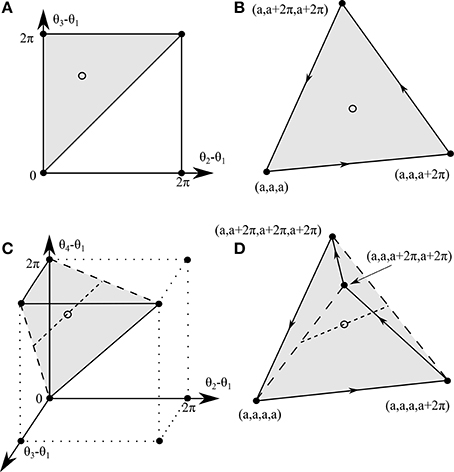
Figure 1. Structure of the canonical invariant region ${C}$ for N = 3 and N = 4. (A,C) show ${C}$ (shaded) in terms of the phase differences θ_j − θ₁ and (B,D) as an orthogonal projection of the diagonal into ℝ² and ℝ³, respectively. The edges of ${C}$ for (A,B) and the faces of ${C}$ for (C,D) are points with S₂ isotropy. The filled circles represent different points on the lift that that correspond to fully synchrony on the torus. The open circle represents the splay phase solution in ${C}$. In (C,D) the solid lines have isotropy S₃ × S₁ while the long dashes have isotropy S₂ × S₂. The short dashed lines have isotropy ${({\text{S}}_1)}^2{\times }_s{\mathbb{Z}}_2$—typical points being (a, b, a + π, b + π). In each case there is a residual ℤ_N−1 symmetry indicated by the arrows in (B,D) and (N − 1)! symmetric copies of ${C}$ pack a generating region for the torus.

Within ${C}$ there are representatives of points with all possible symmetry types. Particularly important are ℓ-cluster states which correspond to states where for some partition of N = m₁ + ⋯ + m_ℓ there are precisely m_k oscillators at the same phase, for some ℓ ≥ 2 (the number of clusters) and m_k ≥ 1 (the size of the kth cluster). These correspond to fixed point subspaces for isotropy groups S_m1 × ⋯ × S_mℓ. These are located on the boundary of ${C}$–there are also points with spatio-temporal symmetries ${({\text{S}}_{m_1}\times \cdots \times {\text{S}}_{m_{\ell }})}^M{\times }_s{\mathbb{Z}}_M$ with M > 1 and N = M(m₁ + ⋯ + m_ℓ); see Ashwin and Swift [9]. NB: To simplify notation we omit copies of S₁ when describing cluster states where this is clear from context: for example S₂ for the case N = 4 corresponds to a three cluster state with isotropy group S₂ × S₁ × S₁.

2. Stabilities and Bifurcations of Solutions Forced by Symmetries

We recall from Ashwin and Swift [9] a number of important synchronous solutions that are forced by symmetry, and their bifurcation properties.

2.1. Stability and Bifurcation of Synchronized Solutions

The fully synchronous solution (in-phase oscillation) of Equation (1) is a periodic orbit given by

$\begin{array}{ll}{\Theta }_{\text{sync}}(t)=\left(\theta (t),\dots ,\theta (t)\right)& (14)\end{array}$

where θ(t) = Ω_synct + θ₀ and Ω_sync = ω + g(0).

Lemma 1 ([9]). The fully synchronous solution Θ_sync(t) is linearly stable if and only if

$\begin{array}{ll}{g}^{\prime }(0)<0.& (15)\end{array}$

For general two harmonic coupling (Equation 4) with q = −1, we have g(0) = 2r cos β − cos α and so there is bifurcation to loss of stability of this solution when

$\begin{array}{ll}r=\frac{cos\alpha }{2cos\beta }& (16)\end{array}$

independent of N.

A splay phase solution (rotating wave) is, up to permutation, a periodic orbit of the form

$\begin{array}{ll}{\Theta }_{\text{splay}}(t)=\left(\theta (t),\theta (t)-\frac{2\pi }{N},\dots ,\theta (t)-\frac{(N-1)2\pi }{N}\right)& (17)\end{array}$

where θ(t) = Ω_splayt + θ₀. There are (N − 1)! different splay phase solutions from the possible permutations, but only one in the canonical invariant region ${C}$. Let $i=\sqrt{-1}$.

Lemma 2 ([9]). The splay phase solutions are linearly stable if the real parts of

$\begin{array}{ll}{\displaystyle \sum _{j=1}^N}{g}^{\prime }\left(\frac{2\pi }{N}j\right)(1-{\rho }^{pj})& (18)\end{array}$

are positive for p = 1, …N − 1, where $\rho =exp(\frac{2\pi i}{N})$.

Let ${\eta }_j=g^{\prime }\left(\frac{2\pi }{N}j\right)$ and ${\nu }_p={\rho }^p=exp(\frac{2\pi i}{N}p)$. If Θ = Θ_splay then the matrix given by

$\begin{array}{l}\hfill A_{ii}(\Theta )=\frac{1}{N}{\displaystyle \sum _{j=1}^N}{g}^{\prime }({\Theta }_{j-1}-{\Theta }_{i-1})=\frac{1}{N}{\displaystyle \sum _{j=1}^N}{\eta }_j,\end{array}$

for i = 1, …, N and

$\begin{array}{l}\hfill A_{ij}(\Theta )=-\frac{1}{N}{g}^{\prime }({\Theta }_{j-1}-{\Theta }_{i-1})=-\frac{1}{N}{\eta }_{j-i}\end{array}$

for i, j = 1, …, N, j ≠ i has eigenvalues

$\begin{array}{l}{\lambda }_p(\Theta )=\frac{1}{N}{\displaystyle \sum _{j=1}^N}{\eta }_j(1-{\nu }_p^j)=\frac{1}{N}{\displaystyle \sum _{j=1}^{N-1}}{\eta }_j(1-{\nu }_p^j)\\ =\frac{1}{N}{\displaystyle \sum _{j=1}^{N-1}}{\eta }_j\left(1-cos\left(\frac{2pj\pi }{N}\right)\right)\\ -i\frac{1}{N}{\displaystyle \sum _{j=1}^{N-1}}{\eta }_{j}sin\left(\frac{2pj\pi }{N}\right),p=1,\dots ,N.\end{array}$

Note that ${\nu }_N^j=exp\left(\frac{2\pi i}{N}jN\right)=1$ implies λ_N(Θ) = 0 for any splay phases. The system has [N/2] complex conjugate pairs

$\begin{array}{l}{\lambda }_{N-p}(\Theta )={\lambda }_{-p}(\Theta )={\overline{\lambda }}_p(\Theta ),\end{array}$

in the even–dimensional case ${\lambda }_{N/2}(\Theta )=\frac{1}{N}\sum _{j=1}^{N-1}{g}^{\prime }\left(\frac{2\pi }{N}j\right)\left(1-{(-1)}^j\right)\in ℝ$. Splay states Θ are stable when

$\begin{array}{l}\mathrm{\text{Re}}({\lambda }_p(\Theta ))=\frac{1}{N}{\displaystyle \sum _{j=1}^{N-1}}{g}^{\prime }\left(\frac{2\pi }{N}j\right)\left(1-cos\left(\frac{2pj\pi }{N}\right)\right)<0,\\ p=1,\dots ,N-1.\end{array}$

The system for phase differences near the splay state has an Andronov–Hopf bifurcation (which can be degenerate or multiple) when Re(λ_p(Θ)) = 0 for some index p = 1, …N − 1, p ≠ N/2, and Im(λ_p(Θ)) ≠ 0.

For general two harmonic coupling (Equation 4) this can be expressed as conditions on the parameters q, r, α, β, though note that unlike the synchronous state, this will depend on N in a fairly complex way. The cases for N = 3 and N = 4 are discussed in Section 3.

2.2. Antiphase States: the Set with Zero Order Parameter.

We discuss briefly a set that is a union of invariant manifolds for some forms of coupling or for small enough N. We note that it is not invariant for generalized coupling N ≥ 5. Consider the Kuramoto order parameter for system (Equation 1) is

$\begin{array}{l}Rexp(i\psi )=\frac{1}{N}{\displaystyle \sum _{k=1}^N}exp(i{\theta }_k)\end{array}$

and define the set with zero order parameter R = 0 by

$\begin{array}{l}{M}^{(N)}=\left\{({\theta }_1,\dots ,{\theta }_N)|{\displaystyle \sum _{k=1}^N}exp(i{\theta }_k)=0\right\}.\end{array}$

This set M^(N) is union of (N − 2)-dimensional manifolds in 𝕋^N [17]; it can be characterized by the set where two variables are given in terms of the other N − 2 variables by expressions

$\begin{array}{l}{\theta }_N=arctan\left(\frac{f_2}{f_1}\right)+\frac{1}{2}arccos\left(\frac{f_1^2+f_1^2}{2}-1\right)\\ +\frac{\pi }{2}(1-\text{sign}(f_1)),\\ {\theta }_{N-1}=arctan\left(\frac{f_2}{f_1}\right)-\frac{1}{2}arccos\left(\frac{f_1^2+f_1^2}{2}-1\right)\\ +\frac{\pi }{2}(1-\text{sign}(f_1)),\end{array}$

where

$\begin{array}{ll}\hfill f_1=-{\displaystyle \sum _{j=2}^N}cos{\theta }_j,& \hfill f_2=-{\displaystyle \sum _{j=2}^N}sin{\theta }_j.\end{array}$

The manifolds can be written in phase differences (for example φ_i = θ₁ − θ_i, i = 1, …N − 1) is (N − 3)–dimensional set in phase space 𝕋^N−1.

Proposition 1 ([26, Lemma 1]). If the coupling function has only one harmonic, for any N the set M^(N) is dynamically invariant; moreover it consists of solutions with fixed phase differences of Equation (1).

However, although some solutions (in particular, splay states Equation 17) belong to M^(N) for arbitrary coupling function and arbitrary g, quite surprisingly it is not generally invariant for general coupling.

Proposition 2. The set M^(N) is invariant for the system (Equation 1) for arbitrary coupling function g(φ) when N = 2, 3, 4 (ω = 0), but not in general for N ≥ 5.

Proof. For N = 2, the equation exp(iθ₁) + exp(iθ₂) = 0 has solution θ₂ = θ₁ + π, while for N = 3, the equation $\sum _{k=1}^{3}exp(i{\theta }_k)=0$ has solution ${\theta }_2={\theta }_1+\frac{2\pi }{3}$, ${\theta }_3={\theta }_1-\frac{2\pi }{3}$. Both cases correspond to the splay phase state which is a zero dimensional fixed point subspace for the phase differences—hence it is dynamically invariant. For N = 4, the equation $\sum _{k=1}^{4}exp(i{\theta }_k)=0$ has solution θ₃ = θ₁ + π, θ₄ = θ₂ + π. This corresponds to the fixed point subspace of ${({\text{S}}_1\times {\text{S}}_1)}^2{\times }_s{\mathbb{Z}}_2$ which is also therefore invariant.

On the other hand, in the case N ≥ 5 the corresponding sets M^(N) are not fixed point subspaces, and therefore not necessarily invariant. For example, the set M⁽⁵⁾ includes points of the form

$\theta =\left({\theta }_1,{\theta }_1+\frac{2\pi }{3},{\theta }_1+\frac{4\pi }{3},{\theta }_4,{\theta }_4+\pi \right)$

which is a two dimensional subspace on which

$R=e^{i{\theta }_1}(1+e^{2i\pi /3}+e^{4i\pi /3})+e^{i{\theta }_4}(1+e^{i\pi })=0.$

However, the smallest fixed point subspaces the contains all points of this form is the trivial subspace 𝕋⁵, meaning the symmetry does not force invariance of M⁽⁵⁾. □

Note that for N = 4 coupled oscillators, the set

$M^{(4)}=\left\{(0,\phi ,\pi ,\phi +\pi ),(0,\pi ,\phi ,\phi +\pi ),(0,\phi ,\phi +\pi ,\pi )\right\}$

(one half-line in each invariant region) as a union of invariant manifolds that correspond to the states with isotropy ℤ₂.

2.3. Stability and Bifurcation of Two Cluster States

Consider any two-cluster states with isotropy S_p × S_{N − p} given by

$\begin{array}{ll}{\Theta }_{p,q}(t)=\left({\theta }_a(t),\dots ,{\theta }_a(t),{\theta }_b(t),\dots ,{\theta }_b(t)\right)& (19)\end{array}$

such that θ_i = θ_a(t) for i = 2, …, p and θ_i = θ_b(t) for i = p + 1, …, N. If we denote φ_p = θ_a − θ_b then (see for example Orosz et al. [27] for the general case) Equation (1) gives

$\begin{array}{l}{\displaystyle \sum _{j=1}^N}g({\theta }_i-{\theta }_j)=\{\begin{array}{l}pg(0)+(N-p)g({\phi }_p),i=1,\dots ,p,\\ pg(-{\phi }_p)+(N-p)g(0),i=p+1,\dots ,N.\end{array}\end{array}$

In this phase difference coordinate we can write

$\begin{array}{rc}\frac{d{\phi }_p}{dt}=pg(0)+(N-p)g({\phi }_p)-pg(-{\phi }_p)-(N-p)g(0).& (20)\end{array}$

Any fixed point in the phase differences will therefore satisfy

$\begin{array}{ll}(2p-N)\left[g(0)-g_{+}({\phi }_p)\right]+N{g}_{-}({\phi }_p)=0.& (21)\end{array}$

For general two harmonic coupling (Equation 4) this means that

$\begin{array}{l}0=(2p-N)\left[g(0)-g_{+}({\phi }_p)\right]+N{g}_{-}({\phi }_p)\\ =(2p-N)\left(cos({\phi }_p)-1\right)\left[qsin\alpha +2rsin\beta \left(cos({\phi }_p)+1\right)\right]\\ +Nsin({\phi }_p)\left[qcos\alpha +2rcos({\phi }_p)cos\beta \right]=0& (22)\end{array}$

This has a trivial solution: the synchronous state with φ_p = 0. Removing the factor of sin(φ_p/2) this means the nontrivial two-cluster states will have a phase difference φ_p where

$\begin{array}{l}0=(N-2p)sin({\phi }_p/2)\left[qsin\alpha +4rsin\beta {cos}^2({\phi }_p/2)\right]\\ \hfill +Ncos({\phi }_p/2)\left[qcos\alpha +2rcos\beta \left(2{cos}^2({\phi }_p/2)-1\right)\right].& (23)\end{array}$

Note that two cluster-states for g(φ) = −sin(φ − α) (i.e., the special case r = 0) are considered in Burylko and Pikovsky [26][Equation 17]. By setting τ = tanφ_p/2, then Equation (23) can be expressed as a cubic equation. If we write p = NP so that 0 < P < 1, this implies the bifurcations occur precisely when the cubic equation for τ

$\begin{array}{l}(1-2P)\left[qsin\alpha \right]{\tau }^3+\left[qcos\alpha -2rcos\beta \right]{\tau }^2\\ +(1-2P)\left[qsin\alpha +4rsin\beta \right]\tau \hfill \\ +\left[qcos\alpha +2rcos\beta \right]=0& (24)\end{array}$

has discriminant zero, namely when

$\begin{array}{ll}0=a_0+a_{1}P+a_2{P}^2+a_3{P}^3+a_4{P}^4,& (25)\end{array}$

where a_k are polynomials in q, r, and cos and sin of α and β. The expressions for the a_k are given in Appendix A (Supplementary Material).

There are also bifurcations with fixed points of two-cluster manifold that occur in transversal to this manifold direction: these create three-cluster states. For example, pitchfork bifurcations (bifurcation line ID in Ashwin et al. [17], Figure 1 for three oscillators can occur transverse to the lines φ₁ = 0 (or φ₂ = 0, φ₁ = φ₂). Such bifurcations cannot be found by examination just of the equation on invariant manifold (Equation 20) or (Equation 21) but need to consider the transverse eigenvalues of the solutions, expressions for which are given in Orosz et al. [27]. Later on we use numerical path following to locate these.

3. Bifurcation Scenarios for Low N and Two Harmonic Coupling

We review and extend the exploration of parameter space of Equation (1) with general two harmonic coupling Equation (4) from the special case β = 0 [17] for N = 3 and N = 4 to more general β ≠ 0.

3.1. Bifurcations for N = 3

Figure 2 illustrates the bifurcations that determine the structure of the phase space for N = 3 in the case q = −1, on varying α ∈ [0, π) and r ≥ 0, for four choices of β. Note that the case β = 0 in the dot-dashed region corresponds to the case considered in Ashwin et al. [17]. Some of the curves are calculated analytically while the remainder of the curves on Figure 2 are obtained by numerical path following of bifurcations in the reduced system (Equation 11) using XPPAUT [28].

FIGURE 2

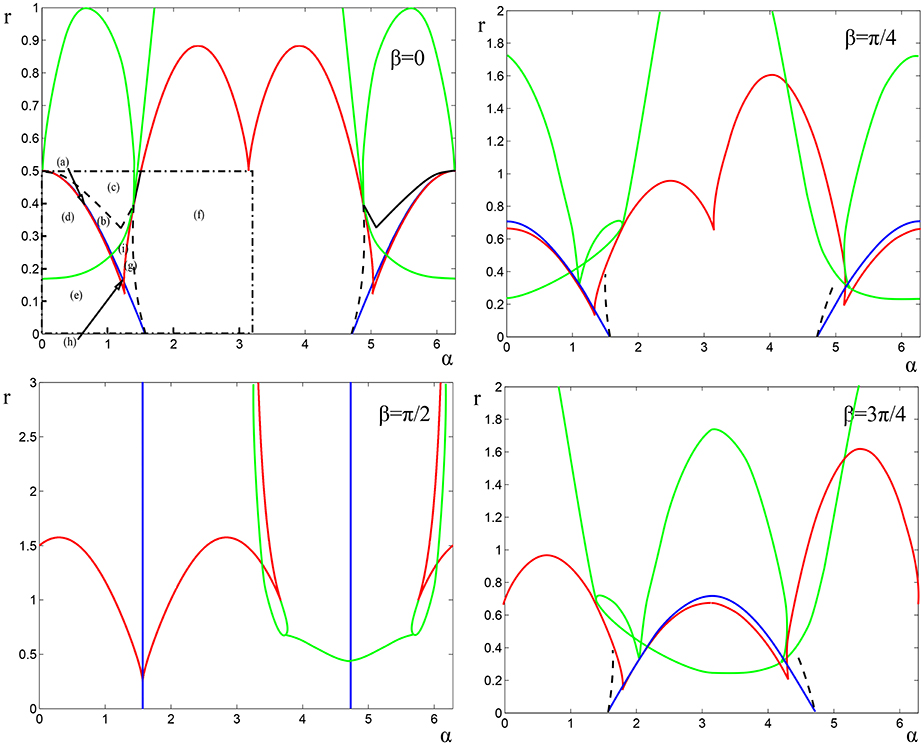
Figure 2. Summary of bifurcations for N = 3 on varying α and r for four choices of β. The blue lines (Equation 16) indicate (simultaneous) steady bifurcation of in-phase and Hopf bifurcation of splay phase solutions. The red lines (Equation 28) indicate saddle-node bifurcations of non-trivial S₂ states. The green lines (found using XPPAUT) give the location of steady bifurcations involving equilibria where all phase differences are non-zero. The black dashed lines indicate homoclinic/heteroclinic bifurcations of periodic solutions. The letters (a–i) show the location of points corresponding to the phase planes shown in Figure 3. The dot-dashed regions for the case β = 0 corresponds to the diagram detailed in Ashwin et al. [17]. Note that in the case β = π/2 and α = π/2 or 3π/2 the system is integrable, while the case β = 3π/4 can be found from that for π/4 by the phase-and time-reversal symmetry (r, α, β) ↦ (r, π − α, π − β).

FIGURE 3

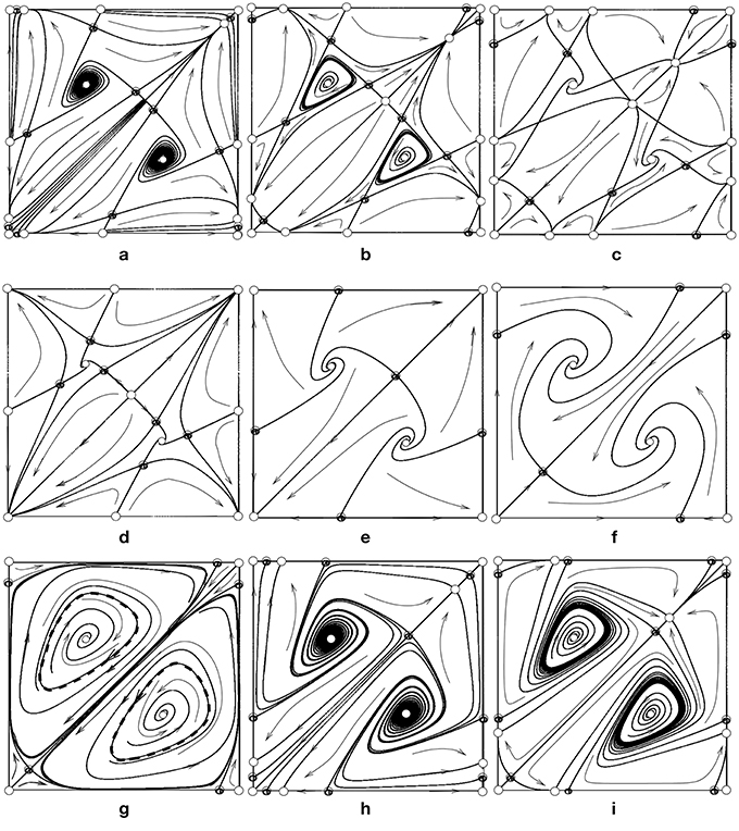
Figure 3. Phase portraits for N = 3 and β = 0, displayed as in Figure 1A on varying α and r, at the locations indicated by (a–i) in Figure 2. The transitions and codimension two points are described in detail in Ashwin et al. [17].

Note that from the previous section, we know that the in-phase solution undergoes bifurcation at (Equation 16). The splay phase solution with N = 3 the stability is governed by the eigenvalues

$\begin{array}{ll}{\lambda }_{\text{splay},N=3}=-\frac{1}{2}qcos\alpha +rcos\beta \pm i\left[\frac{1}{2}qsin\alpha -rsin\beta \right]& (26)\end{array}$

meaning there is a Hopf bifurcation of the splay phase also at

$\begin{array}{l}r=\frac{cos\alpha }{2cos\beta }.\end{array}$

This is precisely the same location as (Equation 16)—a non-generic phenomenon! For N = 3 there is only one type of two-cluster state: this is for p = 1. Setting P = 1/3 and q = −1, (Equation 23) can be expressed as the cubic equation for τ = tan(φ/2):

$\begin{array}{l}-sin\left(\alpha \right){\tau }^3-3\left(2cos\left(\beta \right)r+cos\left(\alpha \right)\right){\tau }^2\\ +\left(4sin\left(\beta \right)r-sin\left(\alpha \right)\right)\tau +6cos\left(\beta \right)r-3cos\left(\alpha \right)=0(27)\end{array}$

which has bifurcations of solutions precisely when the discriminant is zero: this implies the bifurcations of two-cluster states occur when

$\begin{array}{ll}\hfill \begin{array}{ll}0\hfill & =576\left(9{cos}^2\beta +{sin}^2\beta \right){cos}^2\beta r^4\hfill \\ \hfill & +64(36sin\alpha {cos}^2\beta sin\beta +9cos\alpha cos\beta {sin}^2\beta \hfill \\ \hfill & +4sin\alpha {sin}^3\beta +81cos\alpha {cos}^3\beta )r^3\hfill \\ \hfill & +16(9{cos}^2\alpha {sin}^2\beta -99{sin}^2\alpha {cos}^2\beta \hfill \\ \hfill & -12{sin}^2\alpha {sin}^2\beta -18sin\alpha cos\alpha cos\beta sin\beta )r^2\hfill \\ \hfill & +16(63{sin}^2\alpha cos\alpha cos\beta -45sin\alpha cos{\alpha }^{2}sin\beta \hfill \\ \hfill & -81{cos}^3\alpha cos\beta +3{sin}^3\alpha sin\beta )r\hfill \\ \hfill & -4({sin}^4\alpha +16{sin}^2\alpha {cos}^2\alpha +81{cos}^4\alpha ).\hfill \end{array}& (28)\end{array}$

We summarize the bifurcations for β ≠ 0 in Figure 2. One of the more surprising observations of the analysis above can be summarized as follows.

Corollary 1. In order for the Hopf bifurcation of splay phase and the bifurcation of in-phase to occur at different points in parameter space for Equation (1) with N = 3, it is necessary to have a coupling function g with at least three harmonics.

3.2. Bifurcations for N = 4

Figure 4 illustrates a selection of the local bifurcations that determine the structure of the phase space for N = 4 in the case q = −1 on varying α ∈ [0, π) and r ≥ 0 for four values of β. Note that the case β = 0 in the dot-dashed region corresponds to the case considered in Ashwin et al. [17] for N = 4. As before, the in-phase solution has a bifurcation at locations where (Equation 16) is satisfied. For the splay phase solution with N = 4 the stability transverse to the rotating block (0, π, θ, θ + π) is governed by the complex eigenvalues

$\begin{array}{ll}{\lambda }_{\text{splay},N=4}^{(1)}=-\frac{1}{2}qcos\alpha -\frac{i}{2}qsin\alpha & (29)\end{array}$

meaning there is a Hopf bifurcation of the splay phase when cos α = 0, namely at α = π/2 independent of β. There can also be bifurcation from splay phase to rotating block where

$\begin{array}{ll}{\lambda }_{\text{splay},N=4}^{(2)}=-2rcos\beta ,& (30)\end{array}$

meaning there is a bifurcation from the splay phase to rotating blocks (0, π, θ, θ + π) when cos β = 0.

FIGURE 4

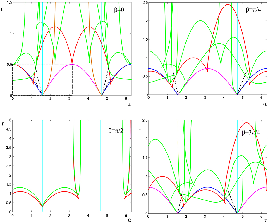
Figure 4. Summary of bifurcations for N = 4 on varying α and r for four choices of β. The blue lines indicate steady bifurcation of the in-phase (Equation 16) while the cyan lines indicate Hopf bifurcation of splay phase solutions (cosα = 0). The red lines indicate saddle-node bifurcations of two cluster states with isotropy S₃. The green lines indicate the location of steady bifurcations involving three cluster states with isotropy S₂. The dashed lines indicate (incomplete lines of) bifurcations of periodic orbits. The dot-dashed regions for the case β = 0 corresponds to the diagram in Ashwin et al. [17]—see there for more details of the dynamics in this case. Note that the case β = π/2 and α = π/2 (or 3π/2) correspond to an even coupling function.

The dynamics of the points with isotropy (S₁ × S₁) × _sℤ₂ (rotating blocks (0, π, θ, θ + π)) is determined by

$\begin{array}{l}\dot{\theta }=4rcos\theta sin(\theta -\beta )\end{array}$

meaning this is degenerate for β = π/2, independent of α! Note that the bifurcations for the rotating blocks only becomes non-degenerate on addition of the fourth harmonic—only then can we get nontrivial solutions with this symmetry. There are two possible two-cluster state: for N = 4 and p = 1 so that P = 1/4 and setting q = −1, (Equation 23) can be expressed as the cubic equation

$\begin{array}{l}-sin(\alpha )t^3-4cos(\beta )r{t}^2-2cos(\alpha )t^2+4sin(\beta )rt\\ -sin(\alpha )t+4cos(\beta )r-2cos(\alpha )=0.\hfill & (31)\end{array}$

There are bifurcations of two cluster states with isotropy S₃ when the discriminant of Equation (31) (not shown here) is zero.

For isotropy S₂ × S₂ we can set N = 4, p = 2 and q = −1 in Equation (23) to find a quadratic expression

$\begin{array}{ll}-2cos\left(\beta \right)r{t}^2-cos\left(\alpha \right)t^2+2cos\left(\beta \right)r-cos\left(\alpha \right)=0& (32)\end{array}$

with discriminant

$\begin{array}{ll}16{\left(cos\left(\beta \right)\right)}^2{r}^2-4{\left(cos\left(\alpha \right)\right)}^2=0.& (33)\end{array}$

Hence the bifurcations of these states are at

$\begin{array}{ll}r=\pm \frac{cos\alpha }{2cos\beta }.& (34)\end{array}$

The remainder of the curves on Figure 4 are obtained by numerical path following of local bifurcations on the two dimensional fixed point subspace of S₂ in the reduced system (Equation 11) using XPPAUT [28]. We remark there may well be more local bifurcations that involve fully symmetry broken (four-cluster) states, as well as global bifurcations that are not shown on this diagram.

4. Dynamics for Odd and Even Coupling Functions

In the case that the coupling function g in Equation (1) is even or odd, the system has additional structure. Write g = g₊ + g₋ where

$\begin{array}{lll}\hfill g_{+}(\phi )=\frac{1}{2}\left(g(\phi )+g(-\phi )\right),& \hfill g_{-}(\phi )=\frac{1}{2}\left(g(\phi )-g(-\phi )\right).& (35)\end{array}$

are the even and odd parts respectively. For the coupling functions of the form (Equation 4) we have

$\begin{array}{ll}\hfill g_{+}(\phi )=-qcos(\phi )sin(\alpha )-rcos(2\phi )sin(\beta ),& (36\text{a})\end{array}$

$\begin{array}{ll}\hfill g_{-}(\phi )=qsin(\phi )cos(\alpha )+rsin(2\phi )cos(\beta ).& (36\text{b})\end{array}$

The remaining results in this section are independent of N and apply to general even or odd g.

If g is odd (i.e., g₊(φ) ≡ 0) then the system for phase differences is a gradient system [10, 29]. More precisely, if we write G′(φ) = g(φ) which is single-valued if g is odd and periodic, we can define a potential

$V(\theta )=-\frac{1}{2N}{\displaystyle \sum _{k,j=1}^N}G({\theta }_k-{\theta }_j)$

then Equation (1) can be written in the form

$\frac{d}{dt}{\theta }_k=\omega -\frac{\partial }{\partial {\theta }_k}V(\theta ).$

This can be seen as a gradient system for the phase differences (Equation 11) on identifying 𝕋^{N − 1} as the set θ ∈ 𝕋^N such that $\sum _k{\theta }_k=0$.

Hence, the only have attractors that are local minima of the potential V. In general, for ω ≠ 0 one can write a potential for the full system on ℝ^N but note that this is multivalued on 𝕋^N.

The case where the coupling function g is even (g₋ ≡ 0) is dynamically more interesting: there are hints that it organizes the emergence of chaotic dynamics for nearby parameter values [22].

Lemma 3. If g is even then the flow of Equation (1) is divergence free. Moreover, the reduced system (Equation 11) is also divergence free.

Proof. To see this, consider

$\frac{\partial F_k}{\partial {\theta }_k}=\frac{1}{N}{\displaystyle \sum _{j\ne k}}g\prime ({\theta }_k-{\theta }_j)$

and so

${\displaystyle \sum _{k=1}^N}\frac{\partial F_k}{\partial {\theta }_k}={\displaystyle \sum _{k=1}^N}{\displaystyle \sum _{j\ne k}}g\prime ({\theta }_k-{\theta }_j).$

Since g is even, this implies that g′ is odd. Thus, $g^{\prime }({\theta }_k-{\theta }_j)=-g^{\prime }({\theta }_j-{\theta }_k)$ and we have

${\displaystyle \sum _{k=1}^N}\frac{\partial F_k}{\partial {\theta }_k}=0.$

More than this, note that the Jacobian in the direction of the 𝕋 action is trivial, meaning that the dynamics of the phase differences (Equation 11) transverse to this direction is also divergence free. □

Recall that an involution ${R}$ : 𝕋^N → 𝕋^N is a time-reversal symmetry if

$\frac{d}{dt}{R}(\theta )=-F({R}(\theta )),$

that is, ${R}$ maps any solution to another solution with the direction of the flow is inverted [13].

Lemma 4. If g is even then the system (Equation 1) has a time and parameter-reversal symmetry ${R}$ : 𝕋^N → 𝕋^N where

${R}(\theta )=-\theta ,\omega \mapsto -\omega ,t\mapsto -t.$

For the reduced system (Equation 11) this corresponds to a time-reversal symmetry $\tilde{{R}}:{𝕋}^{N-1}\to {𝕋}^{N-1}$ where

$\tilde{{R}}(\theta )=-\theta ,t\mapsto -t.$

Proof. Note that for ω = 0 we have

$\begin{array}{l}{F}_k({\theta }_1,\dots ,{\theta }_N)=\frac{1}{N}{\displaystyle \sum _{j=1}^N}g({\theta }_k-{\theta }_j)\\ =\frac{1}{N}{\displaystyle \sum _{j=1}^N}g(-{\theta }_k+{\theta }_j)=F_k(-{\theta }_1,\dots ,-{\theta }_N).\end{array}$

At the same time,

$\frac{d}{dt}{R}(\theta )=-\frac{d\theta }{dt}$

which implies that ${R}$ is a time-reversal symmetry of Equation (1) for the special case ω = 0. This immediately implies that there is a time-reversal symmetry of Equation (11) in general, but only a time and parameter reversal symmetry in general for Equation (1). □

Note that given any symmetry g ∈ Γ and a time-reversal symmetry ${R}$, the composition of the two ${R}$°g is also a time-reversal symmetry. In fact, the set of time-reversal symmetries on 𝕋^N−1 is in one-to-one correspondence with the set of symmetries Γ [13] and can be generated in this way: given any time-reversal symmetry ${R}$, the set of time-reversal symmetries is ${R}$Γ. A consequence is that if θ ∈ 𝕋^N has isotropy H ⊂ S_N × 𝕋 then so does ${R}$(θ).

If ${R}$ is a time reversal-symmetry, the fixed point subspace Fix(${R}$) = {θ ∈ 𝕋^N | ${R}$θ = θ} is not necessarily dynamically invariant, but it is of interest as it yields a natural way to find families of periodic solutions and homoclinic and heteroclinic orbits [13]. In particular, the reversible Lyapunov Centre Theorem asserts that, subject to nonresonance conditions, near an equilibrium in Fix(${R}$) with pairs of purely imaginary eigenvalues there is a two parameter family of reversible periodic orbits, even if there are additional zero eigenvalues [30, 31].

There is a particular time-reversal symmetry $\hat{{R}}:{𝕋}^{N-1}\to {𝕋}^{N-1}$ that maps the canonical invariant region ${C}$ to itself. More precisely, let us define

$\begin{array}{ll}\hfill \hat{{R}}(0,{\theta }_2,\dots ,{\theta }_N)=(0,2\pi -{\theta }_N,\dots ,2\pi -{\theta }_2).& (37)\end{array}$

on the canonical invariant region and note that this is a reversing symmetry corresponding to reversing the order of the components and composing with ${R}$. We characterize all points in ${C}$ that are mapped to themselves by a reversing symmetry. Thus, we define

$\begin{array}{ll}{RC}:=\{\theta \in {C}|{\tau }^q\theta =\hat{{R}}\theta \mathrm{\text{ for some }}q=0,\dots ,N-1\}& (38)\end{array}$

These are the fixed points of time-reversal symmetries within ${C}$. Let us define

$\begin{array}{ll}{Q}^{N,q}:=\{\theta \in {C}|\hat{{R}}\circ {\tau }^{-q}\theta =\theta \}& (39)\end{array}$

and note that

$\begin{array}{ll}{RC}={\displaystyle \bigcup _{q=0}^{N-1}}{Q}^{N,q}.& (40)\end{array}$

On ∂${C}$ we have for $\theta \in {\left\{0,\pi \right\}}^N\cap \overline{{C}}\subset {RC}$. Moreover, the splay state (Equation 17) is contained in ${R}$${C}$. We now turn to the time-reversal symmetries for N = 3 and N = 4 oscillators. In each case we rescale time by N for simplicity.

4.1. Dynamics for Even Coupling Functions: N = 3

A system for N = 3 oscillators has and additional degeneracy: there is a constant of motion

$\begin{array}{ll}V(\theta )=G({\theta }_1-{\theta }_2)+G({\theta }_2-{\theta }_3)+G({\theta }_3-{\theta }_1)& (41)\end{array}$

with G′ = g which generalizes a specific case of the Watanabe–Strogatz constant of motion [21, 32]. Hence, the dynamics of the system is effectively one-dimensional.

For the relative fixed point sets of the time-reversal symmetry, we have

$\begin{array}{ll}\hfill Q^{3,0}=\left\{(0,{\theta }_2,2\pi -{\theta }_2)|{\theta }_2\in (0,\pi )\right\}& (42\text{a})\end{array}$

$\begin{array}{ll}\hfill Q^{3,1}=\left\{(0,{\theta }_2,\pi +{\theta }_2/2)|{\theta }_2\in (0,\pi )\right\}& (42\text{b})\end{array}$

$\begin{array}{ll}\hfill Q^{3,2}=\left\{(0,{\theta }_2,2{\theta }_2)|{\theta }_2\in (0,\pi )\right\}& (42\text{c})\end{array}$

which define three line segments that meet at the splay state. The configurations of the oscillators are depicted in Figure 5. Figure 6 shows ${R}$${C}$ = Q^{N, 0} ∪ Q^{N, 1} ∪ Q^{N, 2} superimposed on the dynamically invariant curves determined by the level sets of Equation (41) for an even coupling function with four Fourier modes:

$\begin{array}{ll}g(\phi )={\displaystyle \sum _{j=0}^4}{c}_{j}cos(j\phi ).& (43)\end{array}$

FIGURE 5

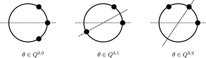
Figure 5. Configurations of phases of three oscillators that are invariant under reflections. Phases 0 = θ₁ < θ₂ < θ₃ are aligned anticlockwise around the circle and the ℤ₃ symmetry operates by rotating the operators anticlockwise by a common phase shift until θ₃ = 0 (and then relabeling oscillators). For Q^{3, q}, reflection along the dashed line corresponds to $\theta \mapsto \hat{{R}}{\tau }^{-q}(\theta )$.

FIGURE 6

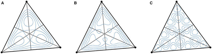
Figure 6. For N = 3 oscillators, the points of ${R}$${C}$ organize the dynamics in ${C}$ for even coupling functions. As in Figure 1B, the boundary of ${C}$ are points of S₂ (black lines) which intersect in Θ_sync (black dot). The union of fixed point subspaces ${R}$${C}$ for time-reversal symmetries are depicted by gray lines which intersect in Θ_splay. The level curves (blue lines) of the constant of motion (Equation 41) for different parameter values of the coupling function (Equation 43) are superimposed in each panel: the nontrivial Fourier coefficients are c₁ = 1, c₂ = 1 in (A), c₁ = −2, c₂ = −2, c₃ = −1, and c₄ = −0.88 in (B), and c₁ = −2, c₂ = −2, c₃ = −1, and c₄ = 10 in (C). Note that in the third panel we are close to an additional symmetry: a high order Fourier component dominates.

The points with time-reversal symmetry ${R}$${C}$ intersect the boundary of the canonical invariant region at (0, 0, 0), (0, 0, π), (0, π, π).

To find the equilibria in ${R}$${C}$ it suffices to evaluate the equilibria in Q^{3, 0} since Q^{3, 1}, Q^{3, 2} are the images of Q^{3, 0} under the action of ℤ₃. Write ψ_k = θ_k − θ₁ and $F_k^{\psi }=F_k-F_1$. On Q^{3, 0} we have the vector field

$\begin{array}{ll}\hfill F_2^{\psi }({\psi }_2,2\pi -{\psi }_2)=g(2{\psi }_2)-g({\psi }_2)& (44\text{a})\end{array}$

$\begin{array}{ll}\hfill F_3^{\psi }({\psi }_2,2\pi -{\psi }_2)=g(2{\psi }_2)-g({\psi }_2)& (44\text{b})\end{array}$

perpendicular to Q^{3, 0}. A point $({\psi }_2^{\star },{\psi }_3^{\star })$ is an equilibrium if $g(2{\psi }_2^{\star })-g({\psi }_2^{\star })=0$ and ${\psi }_3^{\star }=2\pi -{\psi }_2^{\star }$. The linearization of F^ψ at $({\psi }_2^{\star },{\psi }_3^{\star })$,

$\begin{array}{l}D{F}^{\psi }({\psi }_2^{\star },{\psi }_3^{\star })=\\ \left(\begin{array}{cc}g\prime ({\psi }_2^{\star }-{\psi }_3^{\star })& -g\prime ({\psi }_2^{\star }-{\psi }_3^{\star })-g\prime ({\psi }_3^{\star })\\ g\prime ({\psi }_2^{\star }-{\psi }_3^{\star })-g\prime ({\psi }_2^{\star })& -g\prime ({\psi }_2^{\star }-{\psi }_3^{\star })\end{array}\right),& (45)\end{array}$

has eigenvalues

$\begin{array}{l}\lambda =\\ \pm \sqrt{g\prime ({\psi }_2^{\star }-{\psi }_3^{\star })g\prime ({\psi }_2^{\star })-g\prime ({\psi }_2^{\star }-{\psi }_3^{\star })g\prime ({\psi }_3^{\star })+g\prime ({\psi }_2^{\star })g\prime ({\psi }_3^{\star })}\\ =\pm {\left({\displaystyle \sum _{j=1}^3}g\prime ({\theta }_j^{\star }-{\theta }_{j-1}^{\star })g\prime ({\theta }_j^{\star }-{\theta }_{j+1}^{\star })\right)}^{\frac{1}{2}}\end{array}$

where indices are taken modulo N = 3. The eigenvalues thus always take either real or pure imaginary values.

Figure 6 shows examples where it appears that the only equilibria in ${C}$ lie in ${R}$${C}$. Equilibria with a pair of imaginary eigenvalues give rise to “islands” of neutrally stable periodic orbits. These are organized by the stable and unstable manifolds of the saddle points on ${R}$${C}$ which form heteroclinic connections and yield the topological obstructions bounding the islands. The equilibria should relate directly to the constant of motion where the level sets are not smooth manifolds.

4.2. Dynamics for Even Coupling Functions: N = 4

For N = 4 we calculate

$\begin{array}{ll}\hfill Q^{4,0}=\left\{(0,{\theta }_2,\pi ,2\pi -{\theta }_2)|{\theta }_2\in (0,\pi )\right\}& (46\text{a})\end{array}$

$\begin{array}{l}{Q}^{4,1}=\{(0,{\theta }_2,{\theta }_3,2\pi -{\theta }_3+{\theta }_2)\hfill \\ 0<{\theta }_2<{\theta }_3<2\pi -{\theta }_3+{\theta }_2<2\pi \}& (46\text{b})\end{array}$

$\begin{array}{ll}\hfill Q^{4,2}=\left\{(0,{\theta }_2,2{\theta }_2,\pi +{\theta }_2)|{\theta }_2\in (0,\pi )\right\}& (46\text{c})\end{array}$

$\begin{array}{ll}\hfill Q^{4,3}=\left\{(0,{\theta }_2,{\theta }_3,{\theta }_2+{\theta }_3)|0<{\theta }_2<{\theta }_3<{\theta }_2+{\theta }_3<2\pi \right\}.& (46\text{d})\end{array}$

The configuration of phases are depicted in Figure 7. Note that τQ^{4, 0} = Q^{4, 2} and τQ^{4, 1} = Q^{4, 3}. The sets Q^{4, 1}, Q^{4, 3} are subsets of planes that intersect the edges of the canonical invariant in the cluster states with S₂ × S₂ isotropy and lines on the faces corresponding to cluster states with S₂ isotropy. The planes intersect in the interior of the canonical invariant region in the set of points with ℤ₂ isotropy¹ and subdivide the CIR into four connected components. The sets Q^{4, 0}, Q^{4, 2} are line segments that intersect ∂${C}$ in (0, π, π, π), (0, 0, π, 0), (0, 0, 0, π), and (0, π, 0, 0). We have ${\bigcap }_{j=0}^3{Q}^{4,j}={\Theta }_{\text{splay}}$. Figure 8 shows a projection of the canonical invariant region and ${R}$${C}$ for coupling function (Equation 43) with four nontrivial Fourier modes. Note that while ${R}$${C}$ is not necessarily invariant as fixed point subspaces of a time-reversal symmetry, it may contain invariant subsets, such as points of nontrivial isotropy.

FIGURE 7

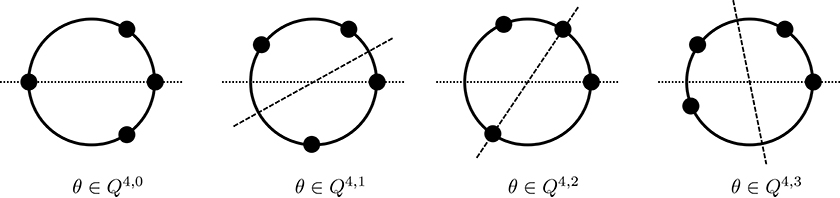
Figure 7. Configurations of phases of four oscillators that are invariant under time-reversal. Phases 0 = θ₁ < θ₂ < θ₃ < θ₄ are aligned anticlockwise around the circle. Reflection along the dashed line for Q^{N, q} corresponds to the action of time-reversal symmetry $\theta \mapsto \hat{{R}}{\tau }^{-q}(\theta )$.

FIGURE 8

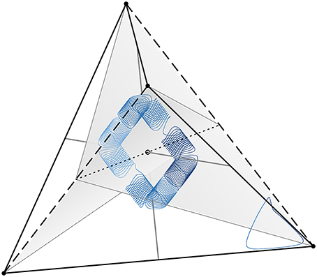
Figure 8. For N = 4 oscillators, the points of ${R}$${C}$ constrain the dynamics in ${C}$ for even coupling functions. As in Figure 1D, the faces of ${C}$ are points of S₂ isotropy and black lines correspond to points of isotropy S₃ (solid), S₂ × S₂ (dashed), and ℤ₂ (dotted). The points in ${R}$${C}$ are depicted in gray: Q^{4, 0}, Q^{4, 2} (thick gray lines), Q^{4, 1}, Q^{4, 3} (planes and thin gray lines that depict points with S₂ isotropy within). Trajectories (blue lines) for two initial conditions are plotted for the coupling function (Equation 43) with coefficients a₁ = −0.5, a₂ = −0.5, a₃ = −0.25, a₄ = 10. The shading of the trajectories indicates in which of the four connected subsets a point lies and changes of color correspond to intersections of the trajectories with Q^{4, 1} and Q^{4, 3}. Note that the trajectories intersect Q^{4, 1} and Q^{4, 3} in exactly two points. For this choice of coupling function a higher order Fourier component dominates as in Figure 6C leading to the “spiraling” motion of the trajectory; details will be discussed elsewhere.

We give equations for fixed points in Q^{4, 0}. In fact, any equilibrium within ${R}$${C}$ for N = 4 oscillators has to be neutrally stable after reducing the phase-shift symmetry; the linearization around equilibria with time-reversing symmetry for a three dimensional system will have one pair of real or pure imaginary eigenvalues and one zero eigenvalue. Introducing phase difference variables ψ_k = θ_k − θ₁ for Q^{4, 0}, we have ψ₃ = π, ψ₄ = 2π − ψ₂. The vector field with components $F_k^{\psi }=F_k-F_1$ is given by

$\begin{array}{ll}\hfill F_2^{\psi }({\psi }_2,\pi ,2\pi -{\psi }_2)=g(2{\psi }_2)+g({\psi }_2+\pi )-g({\psi }_2)-g(\pi ),& (47\text{a})\end{array}$

$\begin{array}{ll}\hfill F_3^{\psi }({\psi }_2,\pi ,2\pi -{\psi }_2)=2(g({\psi }_2+\pi )-g({\psi }_2)),& (47\text{b})\end{array}$

$\begin{array}{ll}\hfill F_4^{\psi }({\psi }_2,\pi ,2\pi -{\psi }_2)=g(2{\psi }_2)+g({\psi }_2+\pi )-g({\psi }_2)-g(\pi ).& (47\text{c})\end{array}$

$\begin{array}{rc}D{F}^{\psi }({\psi }^{\star },\pi ,2\pi -{\psi }^{\star })=\left(\begin{array}{ccc}g\prime ({\psi }^{\star }+\pi )+g\prime (2{\psi }^{\star })& -g\prime ({\psi }^{\star }+\pi )& -g\prime (2{\psi }^{\star })+g\prime ({\psi }^{\star })\\ g\prime ({\psi }^{\star }+\pi )-g\prime ({\psi }^{\star })& 0& -g\prime ({\psi }^{\star }+\pi )+g\prime ({\psi }^{\star })\\ g\prime (2{\psi }^{\star })-g\prime ({\psi }^{\star })& g\prime ({\psi }^{\star }+\pi )& -g\prime (2{\psi }^{\star })-g\prime ({\psi }^{\star }+\pi )\end{array}\right)& (48)\end{array}$

which has eigenvalues

$\begin{array}{rc}\lambda \in \left\{0,\pm \sqrt{\begin{array}{l}2(g\prime ({\psi }^{\star })g\prime ({\psi }^{\star }+\pi )+g\prime ({\psi }^{\star }+\pi )g\prime (2{\psi }^{\star })+\hfill \\ g\prime (2{\psi }^{\star })g\prime ({\psi }^{\star }))-g\prime {({\psi }^{\star })}^2-g\prime {({\psi }^{\star }+\pi )}^2\hfill \end{array}}\right\}& (49)\end{array}$

These simplify if some harmonics of the coupling function g vanish: if the coupling function is π-periodic, g(ϕ + π) = g(ϕ), then Equation (49) yields

$\lambda \in \left\{0,\pm 2\sqrt{g\prime ({\psi }^{\star })g\prime (2{\psi }^{\star })}\right\}$

and if g(ϕ + π) = −g(ϕ) we obtain

$\lambda \in \left\{0,\pm 2ig\prime ({\psi }^{\star })\right\}$

implying that neutrally stable periodic orbits arise nearby.

Note that $F_2^{\psi }=F_4^{\psi }$ along Q^{4, 0}. The linearization of F^ψ at an equilibrium (0, ψ^⋆, π, 2π − ψ^⋆) is

Similarly, one can calculate equilibria in Q^{4, 3} where we have ψ₄ = ψ₂ + ψ₃. For these points, the dynamics are given by

$\begin{array}{ll}\hfill F_2^{\psi }({\psi }_2,{\psi }_3,{\psi }_2+{\psi }_3)=g({\psi }_2-{\psi }_3)-g({\psi }_2+{\psi }_3),& (50\text{a})\end{array}$

$\begin{array}{ll}\hfill F_3^{\psi }({\psi }_2,{\psi }_3,{\psi }_2+{\psi }_3)=g({\psi }_2-{\psi }_3)-g({\psi }_2+{\psi }_3),& (50\text{b})\end{array}$

$\begin{array}{ll}\hfill F_4^{\psi }({\psi }_2,{\psi }_3,{\psi }_2+{\psi }_3)=0.& (50\text{c})\end{array}$

Note that the vector field vanishes in the ψ₄ direction along Q^{4, 3}. Points $(0,{\psi }_2^{\star },{\psi }_3^{\star },{\psi }_2^{\star }+{\psi }_3^{\star })$ are equilibria if

$\begin{array}{ll}g({\psi }_2^{\star }-{\psi }_3^{\star })-g({\psi }_2^{\star }+{\psi }_3^{\star })=0.& (51)\end{array}$

Similarly calculating the eigenvalues, we find

$\begin{array}{ll}\lambda \in \left\{0,\pm \sqrt{\begin{array}{l}2g\prime ({\psi }_2^{\star }-{\psi }_3^{\star })(g\prime ({\psi }_2^{\star })-g\prime ({\psi }_3^{\star }))+2g\prime ({\psi }_2^{\star }+{\psi }_3^{\star })\hfill \\ (g\prime ({\psi }_2^{\star })+g\prime ({\psi }_3^{\star }))\hfill \end{array}}\right\}& (52)\end{array}$

and the eigenvector for λ = 0 is given by

$\begin{array}{ll}{v}_0=\left(\begin{array}{c}g\prime ({\psi }_2^{\star }-{\psi }_3^{\star })+g\prime ({\psi }_2^{\star }+{\psi }_3^{\star })\\ g\prime ({\psi }_2^{\star }-{\psi }_3^{\star })-g\prime ({\psi }_2^{\star }+{\psi }_3^{\star })\\ 2g\prime ({\psi }_2^{\star }-{\psi }_3^{\star })\end{array}\right)& (53)\end{array}$

Since g is even, there are solutions to the fixed point (Equation 51) that are independent of g. The arguments being equal, ${\psi }_2^{\star }-{\psi }_3^{\star }={\psi }_2^{\star }+{\psi }_3^{\star }+2q\pi$, q ∈ ℤ, implies ${\psi }_3^{\star }=q\pi$, q ∈ ℤ and arbitrary ${\psi }_2^{\star }$. If the sign of the arguments is opposite, we have ${\psi }_2^{\star }-{\psi }_3^{\star }=-{\psi }_2^{\star }-{\psi }_3^{\star }+2q\pi$, q ∈ ℤ which implies ${\psi }_2^{\star }=q\pi$, q ∈ ℤ. The condition ${\psi }_3^{\star }=\pi$ defines a line of equilibria given by

$L_{-}=\left\{(0,\phi ,\pi ,\pi +\phi )|\phi \in (0,\pi )\right\}$

which are points of ℤ₂ isotropy in ${C}$. Note that the eigenvector v₀ of the trivial eigenvalue, Equation (53), points along L₋. Moreover, the remaining two eigenvalues evaluate to

$\begin{array}{ll}\lambda =\pm 2\sqrt{g\prime (\phi )g\prime (\phi +\pi )}.& (54)\end{array}$

If some harmonics of the coupling function g vanish they take either real or imaginary values for all points in L₋: if the coupling function is π-periodic, g(ϕ + π) = g(ϕ), L₋ is an continuum of saddles since

$\lambda =\pm 2g\prime (\phi ).$

If g(ϕ + π) = −g(ϕ) we obtain

$\lambda =\pm 2ig\prime (\phi )$

implying that neutrally stable periodic orbits arise close to L₋.

Similarly, in the second case where the sign of the arguments is opposite, consider ${\psi }_2^{\star }=0$ which yields a continuum of equilibria

$L_{+}=\left\{(0,0,\phi ,\phi )|\phi \in (0,2\pi )\right\}$

which are points of S₂ × S₂ isotropy on ∂${C}$. Again, the eigenvector v₀ corresponding to the neutrally stable direction points along L₊. The remaining eigenvalues are given by

$\begin{array}{ll}\lambda =\pm 2g\prime (\phi )& (55)\end{array}$

yielding a family of saddles. The stable and unstable manifolds lie in boundary faces of ${C}$ with S₂ isotropy. They can intersect ${R}$${C}$ again in Q^{4, 1} which intersects the boundary faces adjacent to L₊ in a line.

While the equilibria studied above exist for any choice of even coupling function g, there may be further equilibria that organize the dynamics. First, the Equations (47), (51) may have more equilibria that depend on the coupling function chosen. As these lie in ${R}$${C}$ they have symmetric stability properties. Second, the equilibria that are not contained in ${R}$${C}$ appear to play an important role and yield a mechanism that could give rise to complex heteroclinic networks in the system. For example, assume that θ^⋆ ∈ ${C}$\${R}$${C}$ is a hyperbolic equilibrium with trivial isotropy. Since the vector field is divergence free, the equilibrium has to be a saddle. Suppose that θ^⋆ has one-dimensional stable and two-dimensional unstable manifold. The action of symmetries and time-reversal implies that there are N symmetric copies of θ^⋆. At the same time, there are N copies with inverse stability properties that are given by the group orbit of $\hat{{R}}({\theta }^{\star })$. An intersection of the unstable manifold of θ^⋆ with Q^{4, 1} or Q^{4, 3} yields a heteroclinic connection to an equilibrium related by the time-reversal symmetry. Such a heteroclinic connection may have trivial isotropy (given the way Q^{4, 1} and Q^{4, 3} subdivide the CIR into connected components) or nontrivial isotropy, depending on where this intersection takes place. In this way, a network between the (symmetrically and reversing symmetry related) copies of θ^⋆ may be formed.

5. Discussion

5.1. Even Coupling and Integrability

As noted in Equation (41) for N = 3 and arbitrary even coupling function, there is N − 2 = 1 constant of the motion, in agreement with the case for Kuramoto coupling [15]. It is natural to consider whether there are N − 2 independent constants of the motion for N = 4 and arbitrary even coupling function. If this was the case, the only invariant sets would be two frequency quasiperiodicity. Although Watanabe and Strogatz [15] and the presence of time-reversal symmetries might hints this might be the case, we present evidence there is at most one integral of the motion for N = 4.

In particular, for N = 4 and the states with S₂ isotropy on the boundary of ${C}$, Figure 9 demonstrates that for the case N = 4 and even coupling functions with up to four harmonics of the form (Equation 43) are not fully integrable. In cases (c), (d) of the Figure, we argue there are no nontrivial smooth integrals of the motion within the S₂ subspace, owing to the appearance of sink/source pairs. We only find such evidence of nonintegrable behavior if c₃ and c₄ are non both zero: if c₃ and c₄ are both zero (Equation 43) (only two harmonics) then there are apparently no equilibria within S₂ that are not fixed by a time reversal symmetry and the phase portraits are consistent with the presence of a smooth constant of the motion.

FIGURE 9

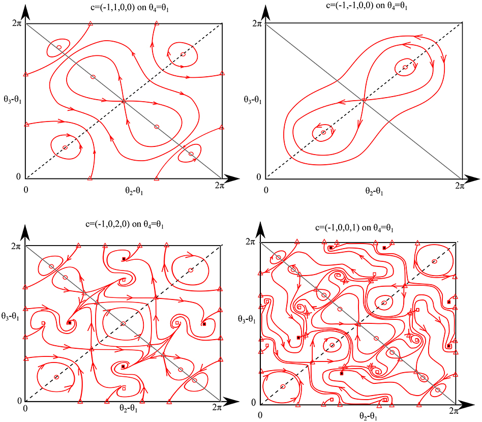
Figure 9. Phase portraits for N = 4 oscillators show a wide range of continua of heteroclinic cycles on the boundary of ${C}$. Here we show a face of the CIR with S₂ isotropy, assuming even g with the first four harmonics given by Equation (43). Dashed black lines are points with S₂ × S₂ isotropy foliated with fixed points and gray lines indicate ${R}$${C}$. For equilibria, triangles are saddles, circles are centers, open squares are sources, and filled squares are sinks; these points are degenerate on the dashed line with S₂ × S₂ isotropy which corresponds to L₊ with transversal stability given by Equation (55). Observe that four our choice of c₁, c₂, all equilibria lie within ${R}$${C}$ if c₃ = c₄ = 0, but there are sink/source pairs (indicating lack of integrability) for cases where one of them is non-zero.

It is still possible that there is one integral of the motion for the case N = 4 and general even coupling, as long as this integral is zero on the boundary of the canonical invariant region, and the trajectory shown in Figure 8 is consistent with this.

5.2. Open Questions

We finish by highlighting some open questions raised in this paper. Firstly, we note that addition of the second harmonic does unfold many degeneracies, though not all. We note that there may be some that are still present for (Equation 1) even for coupling functions with an infinite number of harmonics present, and these will disappear on considering more general coupling that is not of “pairwise” type (see [8]). There seems to be a subtle interplay of the order N, the symmetries of g and the number of harmonics L that determine the dynamics.

Extending a bifurcation analysis to higher N will be harder than extending to higher L, but the latter seems worthwhile especially if it is possible to determine the location of global bifurcations. We do extend the bifurcation analysis here in part analytically, using the special form of the coupling function to write the bifurcations of two-cluster in polynomial form. Potentially this can be extended to more general cluster states, though at the expense of ever more complex expressions. As an alternative approach, rather than doing a bifurcation analysis for fixed L, one could conversely ask whether some harmonics are crucial for specific bifurcations to occur.

The dynamics for the case of an even coupling function shows remarkable subtlety. Numerical experiments show a variety of periodic orbits which can be quite complicated in examples of even coupling functions where a higher harmonic dominates; cf. Figure 8. Although we demonstrate in the previous section that one cannot expect there to be fully integrability with N − 2 independent constants of the motion [15, Theorem, p. 249], there may well be one constant of the motion in the general even coupling case which we have not yet been able to determine.

For even coupling we demonstrate for N = 3, 4 that the set of phases with time-reversal symmetry within the canonical invariant region is a nontrivial (typically noninvariant) set that organizes the dynamics. Complicated dynamics, such as chimera states [23] and chaotic dynamics [22] (and as a consequence also the chaotic weak chimeras constructed in Bick and Ashwin [33]), typically arise in systems for small perturbations away from a system with time-reversal symmetry. We anticipate that understanding these heteroclinic networks in greater detail will shed light on how complicated arise in networks of coupled phase oscillators. Naturally, the more equilibria there are, the more intricate the heteroclinic network can be. Thus, deriving conditions for the existence of equilibria depending on the coupling function seems like a first step to understand the dynamics for even coupling functions g.

Author Contributions

All authors listed, have made substantial, direct and intellectual contribution to the work, and approved it for publication.

Conflict of Interest Statement

The authors declare that the research was conducted in the absence of any commercial or financial relationships that could be construed as a potential conflict of interest.

Acknowledgments

PA gratefully acknowledges the financial support of the EPSRC via grant EP/N014391/1. CB gratefully acknowledges financial support from the People Programme (Marie Curie Actions) of the European Union's Seventh Framework Programme (FP7/2007–2013) under REA grant agreement no. 626111.

Supplementary Material

The Supplementary Material for this article can be found online at: https://www.frontiersin.org/article/10.3389/fams.2016.00007

Footnotes

1. ^Note that for N > 4 there are points with ℤ_k ⊂ ℤ_N isotropy that are not in ${R}$${C}$.

References

1. Winfree A. T. The Geometry of Biological Time, 2nd Edn. New York, NY: Springer (2001). doi: 10.1007/978-1-4757-3484-3

CrossRef Full Text | Google Scholar

2. Kuramoto Y. Chemical Oscillations, Waves and Turbulence. Berlin: Springer-Verlag (1984). doi: 10.1007/978-3-642-69689-3

CrossRef Full Text

3. Kuramoto Y. Self-entrainment of a population of coupled non-linear oscillators. In: Araki H, editor. International Symposium on Mathematical Problems in Theoretical Physics, Lecture Notes in Physics. Berlin: Springer-Verlag (1975). p. 420–422. doi: 10.1007/BFb0013365

CrossRef Full Text

4. Ashwin P, Coombes S, Nicks R. Mathematical frameworks for oscillatory network dynamics in neuroscience. J Math Neurosci. (2016) 6:1–92. doi: 10.1186/s13408-015-0033-6

PubMed Abstract | CrossRef Full Text | Google Scholar

5. Acebrón J, Bonilla L, Pérez Vicente C, Ritort F, Spigler R. The Kuramoto model: a simple paradigm for synchronization phenomena. Rev Mod Phys. (2005) 77:137–85. doi: 10.1103/RevModPhys.77.137

CrossRef Full Text | Google Scholar

6. Strogatz SH. From Kuramoto to Crawford: exploring the onset of synchronization in populations of coupled oscillators. Phys D (2000) 143:1–20. doi: 10.1016/S0167-2789(00)00094-4

CrossRef Full Text | Google Scholar

7. Ullner E, Politi A. Self-sustained irregular activity in an ensemble of neural oscillators. Phys Rev X (2016) 6:011015. doi: 10.1103/PhysRevX.6.011015

CrossRef Full Text | Google Scholar

8. Ashwin P, Rodrigues A. Hopf normal form with S_N symmetry and reduction to systems of nonlinearly coupled phase oscillators. Phys D (2016) 325:14–24. doi: 10.1016/j.physd.2016.02.009

CrossRef Full Text | Google Scholar

9. Ashwin P, Swift JW. The dynamics of n weakly coupled identical oscillators. J Nonlin Sci. (1992) 2:69–108. doi: 10.1007/BF02429852

CrossRef Full Text | Google Scholar

10. Brown E, Holmes P, Moehlis J. Globally coupled oscillator networks. In: Perspectives and Problems in Nonlinear Science: A Celebratory Volume in Honor of Larry Sirovich, eds E. Kaplan, J. E. Marsden, and K. R. Sreenivasan (New York, NY: Springer) (2003). p. 183–215. doi: 10.1007/978-0-387-21789-5_5

CrossRef Full Text | Google Scholar

11. Golubitsky M, Schaeffer DG, Stewart IN. Singularities and Groups in Bifurcation Theory, Vol. II. New York, NY: Springer-Verlag (1988). doi: 10.1007/978-1-4612-4574-2

CrossRef Full Text

12. Sevryuk MB. Reversible Systems. Springer Lecture Notes in Mathematics. Berlin: Springer (1986).

Google Scholar

13. Lamb JSW, Roberts JAG. Time-reversal symmetry in dynamical systems: a survey. Phys D (1998) 112:1–39. doi: 10.1016/S0167-2789(97)00199-1

CrossRef Full Text | Google Scholar

14. Sakaguchi H, Kuramoto Y. A soluble active rotator model showing phase transitions via mutual entrainment. Prog Theor Phys. (1986) 76:576–81. doi: 10.1143/PTP.76.576

CrossRef Full Text | Google Scholar

15. Watanabe S, Strogatz SH. Constants of motion for superconducting Josephson arrays. Phys D (1994) 74:197–253. doi: 10.1016/0167-2789(94)90196-1

CrossRef Full Text | Google Scholar

16. Kori H, Kuramoto Y, Jain S, Kiss IZ, Hudson J. Clustering in globally coupled oscillators near a Hopf bifurcation: theory and experiments. Phys Rev E (2014) 89:062906. doi: 10.1103/PhysRevE.89.062906

CrossRef Full Text | Google Scholar

17. Ashwin P, Burylko O, Maistrenko Y. Bifurcation to heteroclinic cycles and sensitivity in three and four coupled phase oscillators. Phys D (2008) 237:454–66. doi: 10.1103/PhysRevE.89.062906

CrossRef Full Text | Google Scholar

18. Hansel D, Mato G, Meunier C. Clustering and slow switching in globally coupled phase oscillators. Phys Rev E (1993) 48:3470–77. doi: 10.1103/PhysRevE.48.3470

CrossRef Full Text | Google Scholar

19. Ashwin P, Orosz G, Wordsworth J, Townley S. Dynamics on networks of clustered states for globally coupled phase oscillators. SIAM J Appl Dyn Syst. (2007) 6:728–58. doi: 10.1137/070683969

CrossRef Full Text | Google Scholar

20. Daido H. Onset of cooperative entrainment in limit-cycle oscillators with uniform all-to-all interactions: bifurcation of the order function. Phys D (1996) 91:24–66.

Google Scholar

21. Bick C. Chaos and Chaos Control in Network Dynamical Systems. PhD dissertation, Georg-August-Universität Göttingen (2012).

Google Scholar

22. Bick C, Timme M, Paulikat D, Rathlev D, Ashwin P. Chaos in symmetric phase oscillator networks. Phys Rev Lett. (2011) 107:244101. doi: 10.1103/PhysRevLett.107.244101

PubMed Abstract | CrossRef Full Text | Google Scholar

23. Abrams DM, Strogatz SH. Chimera states for coupled oscillators. Phys Rev Lett. (2004) 93:174102. doi: 10.1103/PhysRevLett.93.174102

PubMed Abstract | CrossRef Full Text | Google Scholar

24. Panaggio MJ, Abrams DM. Chimera states: coexistence of coherence and incoherence in networks of coupled oscillators. Nonlinearity (2015) 28:R67–87. doi: 10.1088/0951-7715/28/3/R67

CrossRef Full Text | Google Scholar

25. Laing CR. The dynamics of chimera states in heterogeneous Kuramoto networks. Phys D (2009) 238:1569–88. doi: 10.1016/j.physd.2009.04.012

CrossRef Full Text | Google Scholar

26. Burylko O, Pikovsky A. Desynchronization transitions in nonlinearly coupled phase oscillators. Phys D (2011) 240:1352–61. doi: 10.1016/j.physd.2011.05.016

CrossRef Full Text | Google Scholar

27. Orosz G, Moehlis J, Ashwin P. Designing the dynamics of globally coupled oscillators. Prog Theor Phys. (2009) 122:611–30. doi: 10.1143/PTP.122.611

CrossRef Full Text | Google Scholar

28. Ermentrout GB. A Guide to XPPAUT for Researchers and Students. Pittsburgh, PA: SIAM (2002).

Google Scholar

29. Hoppensteadt FC, Izhikevich EM. Weakly Connected Neural Networks, volume 126 of Applied Mathematical Sciences. New York, NY: Springer (1997). doi: 10.1007/978-1-4612-1828-9

CrossRef Full Text | Google Scholar

30. Devaney RL. Reversible diffeomorphisms and flows. Trans Am Math Soc. (1976) 218:89–113. doi: 10.1090/S0002-9947-1976-0402815-3

CrossRef Full Text | Google Scholar

31. Golubitsky M, Krupa M, Lim C. Time-reversibility and particle sedimentation. SIAM J Appl Math. (1991) 51:49–72. doi: 10.1137/0151005

CrossRef Full Text | Google Scholar

32. Pikovsky A, Rosenau P. Phase compactons. Phys D (2006) 218:56–69. doi: 10.1016/j.physd.2006.04.015

CrossRef Full Text | Google Scholar

33. Bick C, Ashwin P. Chaotic weak chimeras and their persistence in coupled populations of phase oscillators. Nonlinearity (2016) 29:1468–1486. doi: 10.1088/0951-7715/29/5/1468

CrossRef Full Text | Google Scholar