Statistical Data Assimilation: Formulation and Examples From Neurobiology

1. Introduction

A broad class of “inverse” problems presents itself in many scientific and engineering inquiries. The overall question addressed by these is how to transfer information from laboratory and field observations to candidate models of the processes underlying those observations.

The existence of large, information rich, well curated data sets from increasingly sophisticated observations on complicated nonlinear systems has set new challenges to the information transfer task. Assisting with this challenge are new substantial computational capabilities.

Together they have provided an arena in which principled formulation of this information transfer along with algorithms to effect the transfer have come to play an essential role. This paper reports on some efforts to meet this class of challenge within neuroscience. Many of the ideas are applicable much more broadly than our focus, and we hope the reader will find this helpful in their own inquiries.

In this special issue entitled Data Assimilation and Control: Theory and Applications in Life Sciences, of the journal Frontiers in Applied Mathematics and Statistics–Dynamical Systems, we participate in the broader quantitative setting for this information transfer. The procedures are called “data assimilation” following its use in the effort to develop realistic numerical weather prediction models [1, 2] over many decades. We prefer the term “statistical data assimilation” (SDA) to emphasize that key ingredients in the procedures involved in the transfer rest on noisy data and on recognizing errors in the models to which information in the noisy data is to be transferred.

This article begins with a formulation of SDA with some additional clarity beyond the discussion in Abarbanel [3]. We also discuss some algorithms helpful for implementing the information transfer, testing model compatibility with the available data, and quantitatively identifying how much information in the data can be represented in the model selected by the SDA user. Using SDA will also remind us that data assimilation efforts are well cast as problems in statistical physics [4].

After the discussion of SDA, we turn to some working ideas on how to perform the high dimensional integrals involved in SDA. In particular we address the “standard model” of SDA where data is contaminated by Gaussian noise and model errors are represented by Gaussian noise, though the integrals to be performed are, of course, not Gaussian. The topics include the approximation of Laplace [5] and Monte Carlo methods.

With these tools in hand, we turn to neurobiological questions that arise in the analysis of individual neurons and, in planning, for network components of the avian song production pathway. These questions are nicely formulated in the general framework, and we dwell on specifics of SDA in a realistic biological context. The penultimate topic we address is the use of SDA to calibrate VLSI analog chips designed and built as components of a developing instantiation of the full songbird song command network, called HVC. Lastly, we discuss the potential utlization of SDA for exploring biological networks.

At the outset of this article we may expect that our readers from Physics and Applied Mathematics along with our readers from Neurobiology may find the conjunction of the two “strange bedfellows” to be incongruous. For the opportunity to illuminate the natural melding of the facets of both kinds of questions, we thank the editors of this special issue.

2. Materials and Methods

2.1. General Overview of Data Assimilation

We will provide a structure within which we will frame our discussion of transfer of information from data to a model of the underlying processes producing the data.

We start with an observation window in time [t₀, t_F] within which we make a set of measurements at times t = {τ₁, τ₂, …, τ_k, …, τ_F};t₀ ≤ τ_k ≤ t_F. At each of these measurement times, we observe L quantities y(τ_k) = {y₁(τ_k), y₂(τ_k), …, y_L(τ_k)}. The number L of observations at each measurement time τ_k is typically less, often much less, than the number of degrees of freedom D in the observed system; D ≫ L.

These are views into the dynamical processes of a system we wish to characterize. The quantitative characterization is through a model we choose. It describes the interactions among the states of the observed system. If we are observing the time course of a neuron, for example, we might measure the membrane voltage y₁(τ_k) = V_m(τ_k) and the intracellular Ca²⁺ concentration $y_2({\tau }_k)=\left[C{a}^{2+}\right]({\tau }_k)$. From these data we want to estimate the unmeasured states of the model as a function of time as well as estimate biophysical parameters in the model.

The processes characterizing the state of the system (neuron) we call x_a(t);a = 1, 2, …, D ≥ L, and they are selected by the user to describe the dynamical behavior of the observations through a set of equations in continuous time

$\begin{array}{ll}\frac{d{x}_a(t)}{dt}=F_a(\text{x}(t),\text{q}),& (1)\end{array}$

or in discrete time t_n = t₀+nΔt; n = 0, 1, …, N; t_N = t_F via

$\begin{array}{ll}{x}_a(t_{n+1})=x_a(n+1)=f_a(\text{x}(t_n),\text{q})=f_a(\text{x}(n),\text{q}),& (2)\end{array}$

where q is a set of fixed parameters associated with the model. f(x(n), q) is related to F(x(t), q) through the choice the user makes for solving the continuous time flow for x(t) through a numerical solution method of choice [6].

Considering neuronal activity, Equation 1 could be coupled Hodgkin-Huxley (HH) Equations [7, 8] for voltage, ion channel gating variables, constituent concentrations, and other ingredients. If the neuron is isolated in vitro, such as by using drugs to block synaptic transmission, then there would be no synaptic input to the cell to describe. While if it is coupled to a network of neurons, their functional connectivity would be described in F(x(t), q) or f(x(n), q). Typical parameters might be maximal conductances of the ion channels, reversal potentials, and other time-independent numbers describing the kinetics of the gating variables. In many experiments L is only 1, namely, the voltage across the cell membrane, while D may be on the order of 100; Hence D ≫ L.

As we proceed from the initiation of the observation window at t₀ we must move our model equation variables x(0), Equation 2, from t₀ to τ₁ where a measurement is made. Then using the model dynamics we move along to τ₂ and so forth until we reach the last measurement time τ_F and finally move the model from x(τ_F) to x(t_F). In each stepping of the model equations (Equation 2) we may make many steps of Δt in time to achieve accuracy in the representation of the model dynamics. The full set of times t_n at which we evaluate the model x(t_n) we collect into the path of the state of the model through D-dimensional space: X = {x(0), x(1), …, x(n), …, x(N) = x(F)}. The dimension of the path is (N + 1)D + N_q, where N_q is the number of parameters q in our model.

It is worth a pause here to note that we have now collected two of the needed three ingredients to effect our transfer of the information in the collection of all measurements Y = {y(τ₁),y(τ₂), …,y(τ_F)} to the model f(x(n), q) along the path X through the observation window [t₀, t_F]: (1) data Y and (2) a model of the processes in Y, devised by our experience and knowledge of those processes. The notation and a visual presentation of this is found in Figure 1.

FIGURE 1

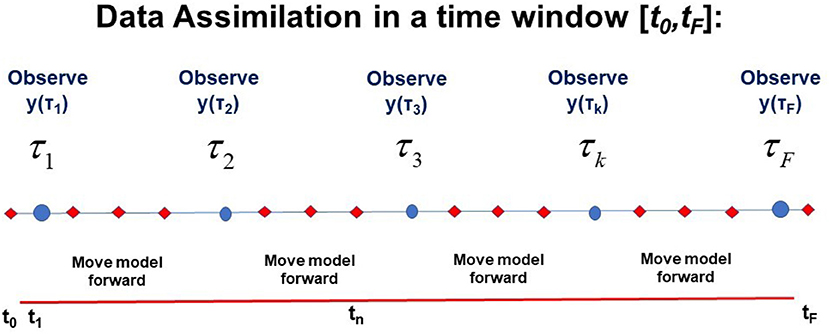
Figure 1. A visual representation of the window t₀ ≤ t ≤ t_F in time during which L-dimensional observations y(τ_k) are performed at observation times t = τ_k; k = 1, …, F. This also shows times at which the D-dimensional model developed by the user x(n+1) =f(x(n), q) is used to move forward from time n to time n+1: t_n = t₀+nΔt; n = 0, 1, …, N. D ≥ L. The path of the model X = {x(0), x(1), …, x(n), …, x(N) = x(F)} and the collection Y of L-dimensional observations at each observation time τ_k, Y = {y(τ₁),y(τ₂), …,y(τ_k), …,y(τ_F} (y = {y₁, y₂, …, y_L}) is also indicated.

The third ingredient, comprised of methods to generate the transfer from Y to properties of the model, will command our attention throughout most of this paper. If the transfer methods are successful and, according to some metric of success, we arrange matters so that at the measurement times τ_k, the L model variables x(t) associated with y(τ_k) are such that x_l(τ_k) ≈ y_l(τ_k), we are not finished. We have then only demonstrated that the model is consistent with the known data Y. We must use the model, completed by the estimates of q and the state of the model at t_F, x(t_F), to predict forward for t > t_F, and we should succeed in comparison with measurements for y(τ_r) for τ_r > t_F. As the measure of success of predictions, we may use the same metric as utilized in the observation window.

As a small aside, the same overall setup applies to supervised machine learning networks [9] where the observation window is called the training set; the prediction window is called the test set, and prediction is called generalization.

2.1.1. The Data Are Noisy; The Model Has Errors

Inevitably, the data we collect is noisy, and equally the model we select to describe the production of those data has errors. This means we must, at the outset, address a conditional probability distribution P(X|Y) as our goal in the data assimilation transfer from Y to the model. In Abarbanel [3] we describe how to use the Markov nature of the model x(n) → x(n+1) =f(x(n), q) and the definition of conditional probabilities to derive the recursion relation:

$\begin{array}{l}P(\text{X}(n+1)|Y(n+1))=\frac{P(y(n+1),\text{x}(n+1),\text{X}(n)|Y(n))}{P(y(n+1)|Y(n))P(\text{x}(n+1),\text{X}(n)|Y(n))}•\\ P(\text{x}(n+1)|\text{x}(n))P(\text{X}(n)|Y(n))\\ =exp\left[CMI(y(n+1),\text{x}(n+1),\text{X}(n)|Y(n))\right]•\\ P(\text{x}(n+1)|\text{x}(n))P(\text{X}(n)|Y(n)),& (3)\end{array}$

where we have identified $CMI(a,b|c)=log\left[\frac{P(a,b|c)}{P(a|c)P(b|c)}\right]$. This is Shannon's conditional mutual information [10] telling us how many bits (for log₂) we know about a when observing b conditioned on c. For us a = {y(n + 1)}, b = {x(n + 1), X(n)}, c = {Y(n)}. We can simplify this further with the assumption that an observation at any time depends only on the state of the system.

$\begin{array}{l}P(\text{X}(n+1)|\text{Y}(n+1))=P(\text{y}(n+1)|\text{X}(n+1))P(\text{x}(n+1)\\ |\text{x}(n))P(\text{X}(n)|\text{Y}(n))& (4)\end{array}$

Using this recursion relation to move backwards through the observation window from t_F = t₀ + NΔt through the measurements at times τ_k to the start of the window at t₀, we may write, up to factors independent of X

$\begin{array}{ll}P(\text{X}|Y)=\left\{{\displaystyle \prod _{k=1}^F}P(y({\tau }_k)|\text{X}({\tau }_k)){\displaystyle \prod _{n=0}^{N-1}}P(\text{x}(n+1)|\text{x}(n))\right\}P(\text{x}(0)).& (5)\end{array}$

If we now write P(X|Y) ∝ exp[−A(X)] where A(X), the negative of the log likelihood, we call the action, then conditional expected values for functions along the path X are defined by

$\begin{array}{ll}E\left[G(\text{X})|Y\right]=\langle G(\text{X})\rangle =\frac{\int d\text{X}G(\text{X})e^{-A(\text{X})}}{\int d\text{X}{e}^{-A(\text{X})}},& (6)\end{array}$

$d\text{X}={\prod }_{n=0}^N{d}^D\text{x}(n)$, and all factors in the action independent of X cancel out here. The action takes the convenient expression

$\begin{array}{l}A(\text{X})=-\{{\displaystyle \sum _{k=1}^F\log }[P(\text{y}({\tau }_k)|\text{X}({\tau }_k)]+\underset{n=0}{\overset{N-1}{\Sigma }}\\ \log [P(\text{x}(n+1)|\text{x}(n))]\}-\log [P(\text{x}(0))],& (7)\end{array}$

which is the sum of the terms which modify the conditional probability distribution when an observation is made at t = τ_k and the sum of the stochastic version of x(n) → x(n + 1) − f(x(n), q) and finally the distribution when the observation window opens at t₀.

What quantities G(X) are of interest? One natural one is the path G(X) = X_μ; μ = {a, n} itself; another is the covariance around that mean $\langle {\text{X}}_{\mu }\rangle ={\bar{\text{X}}}_{\mu }=\langle {\text{X}}_{\mu }\rangle :\langle ({\text{X}}_{\mu }-{\bar{\text{X}}}_{\mu })({\text{X}}_{\nu }-{\bar{\text{X}}}_{\nu })\rangle$. Other moments are of interest, of course. If one has an anticipated form for the distribution at large X, then G(X) may be chosen as a parametrized version of that form and those parameters determined near the maximum of P(X|Y).

The action simplifies to what we call the “standard model” of data assimilation when (1) observations y are related to their model counterparts via Gaussian noise with zero mean and diagonal precision matrix R_m, and (2) model errors are associated with Gaussian errors of mean zero and diagonal precision matrix R_f:

$\begin{array}{l}A(\text{X})={\displaystyle \sum _{k=1}^F}{\displaystyle \sum _{l=1}^L}\frac{R_m(k)}{2}{(x_l({\tau }_k)-y_l({\tau }_k))}^2+{\displaystyle \sum _{n=0}^{N-1}}{\displaystyle \sum _{a=1}^D}\frac{R_f(a)}{2}\\ {(x_a(n+1)-f_a(\text{x}(n),\text{q}))}^2.& (8)\end{array}$

If we have knowledge of the distribution P(x(0)) at t₀ we may add it to this action. If we have no knowledge of P(x(0)), we may take its distribution to be uniform over the dynamic range of the model variables, then it, as here, is absent, canceling numerator and denominator in Equation (6).

Our challenge is to perform integrals such as Equation (6). One should anticipate that the dominant contribution to the expected value comes from the maxima of P(X|Y) or, equivalently the minima of A(X). At such minima, the two contributions to the action, the measurement error and the model error, balance each other to accomplish the explicit transfer of information from the former to the latter.

We note, as before, that when f(x(n), q) is nonlinear in X, as it always is in interesting examples, the expected value integral Equation (6) is not Gaussian. So, some thinking is in order to approximate this high dimensional integral. We turn to that now. After consideration of methods to do the integral, we will return to a variety of examples taken from neuroscience.

The two generally useful methods available for evaluating this kind of high dimensional integral are Laplace's method [5] and Monte Carlo techniques [6, 11, 12]. We address them in order. We also add our own new and useful versions of the methods.

2.1.2. Laplace's Method

To locate the minima of the action A(X) = −log[P(X|Y)] we must seek paths X^(j); j = 0, 1, … such that $\partial A(\text{X})/\partial \text{X}{|}_{{\text{X}}^{(j)}}=0$, and then check that the second derivative at X^(j), the Hessian, is a positive definite matrix in path coordinates. The vanishing of the derivative is a necessary condition.

Laplace's method [5] expands the action around the X^(j) seeking the path X⁽⁰⁾ with the smallest value of A(X). The contribution of X⁽⁰⁾ to the integral Equation (6) is approximately exp[A(X⁽¹⁾) − A(X⁽⁰⁾)] bigger than that of the path with the next smallest action.

This sounds more or less straightforward; however, finding the global minimum of a nonlinear function such as A(X) is an NP-complete problem [13]. In a practical sense one cannot expect to succeed with such problems. However there is an attractive feature of the form of A(X) that permits us to accomplish more.

We now discuss two algorithmic approaches to implementing Laplace's method.

2.1.3. Precision Annealing for Laplace's Method

Looking at Equation (8) we see that if the precision of the model is zero, R_f = 0, the action is quadratic in the L measured variables x_l(n) and independent of the remaining states. The global minimum of such an action comes with x_l(τ_k) = y_l(τ_k) and any choice for the remaining states and parameters. Choose the path with these values of x(τ_k) and values from a uniform distribution of the other state variables and parameters covering the expected dynamic range of those, and call it path X_init. In practice, we recognize that the global minimum of A(X) is degenerate at R_f = 0, so we select many initial paths. We choose N_I of them, and initialize whatever numerical optimization program we have selected, to run on each of them. We continue to call the collection of N_I paths X_init.

• Now we increase R_f from R_f = 0 to a small value R_f0. Use each of the N_I paths in X_init as initial conditions for our numerical optimization program chosen to find the minima of A(X), and we arrive at N_I paths X₀. Evaluate A(X₀) on all N_I paths X₀.

• We increase R_f = R_f0 → R_f0α; α > 1, and now use the N_I paths X₀ as the initial conditions for our numerical optimization program chosen to find the minima of A(X), we arrive at N_I paths X₁. Evaluate A(X₁) on all N_I paths X₁.

• We increase $R_f=R_{f0}\alpha \to R_{f0}{\alpha }^2$. Now use the N_I paths X₁ as the initial conditions for our numerical optimization program chosen to find the minima of A(X), we arrive at N_I paths X₂. Evaluate A(X₂) on all N_I paths X₂.

• Continue in this manner increasing R_f to $R_f=R_{f0}{\alpha }^{\beta };\beta =0,1,\dots$, then using the selected numerical optimization program to arrive at N_I paths X_β. Evaluate A(X_β) on all N_I paths X_β.

• As a function of ${log}_{\alpha }\left[\frac{R_f}{R_{f0}}\right]$ display all N_I values of A(X_β) vs. β for all β = 0, 1, 2, …β_max.

We call this method precision annealing (PA) [14–17]. It slowly turns up the precision of the model collecting paths at each R_f that emerged from the degenerate global minimum at R_f = 0. In practice it is able to track N_I possible minima of A(X) at each R_f. When not enough information is presented to the model, that is L is too small, there are many local minima at all R_f. This is a manifestation of the NP-completeness of the minimization of A(X) problem. None of the minima may dominate the expected value integral of interest.

As L increases, and enough information is transmitted to the model, for large R_f one minimum appears to stand out as the global minimum, and the paths associated with that smallest minimum yields good predictions. We note that there are always paths, not just a single path, as we have a distribution of paths, N_I of which are sampled in the PA procedure, within a variation of size $1/\sqrt{R_m}$. A clear example of this is seen in Shirman [18] in a small, illustrative model.

In the even that the chosen model is inconsistent with the data, or there is too much noise in the model error term, a single minimum of the action will not appear for large R_f. As in the case of too few measurements, there will be multiple local minima. An example of this can be seen in Ye et al. [14].

2.1.4. “Nudging” Within Laplace's Method

In meteorology one approach to data assimilation is to add a term to the deterministic dynamics which move the state of a model toward the observations [19]

$\begin{array}{ll}{x}_a(n+1)=f_a(\text{x}(n),\text{q})+u(n)(y_l(n)-x_l(n)){\delta }_{al},& (9)\end{array}$

where u(n) > 0 and vanishes except where a measurement is available. This is referred to as “nudging.” It appears in an ad hoc, but quite useful, manner.

Within the structure we have developed, one may see that the “nudging term” arises through the balance between the measurement error term and the model error term in the action. This is easy to see when we look at the continuous time version of the data assimilation standard model

$\begin{array}{l}A(\text{x}(t),\dot{\text{x}}(t))={\displaystyle {\int }_{t_0}^{t_F}d}t\{{\displaystyle \sum _{l=1}^L}\frac{R_m(t,l)}{2}{(x_l(t)-y_l(t))}^2\\ +{\displaystyle \sum _{a=1}^D\frac{R_f(a)}{2}}{({\dot{x}}_a(t)-F_a(\text{x}(t),\text{q}))}^2\}.& (10)\end{array}$

The extremum of this action is given by the Euler-Lagrange equations for the variational problem [20]

$\begin{array}{l}\left[{\delta }_{ab}\frac{d}{dt}+\frac{\partial F_b(\text{x}(t)}{\partial x_a(t)}\right]\left[{\dot{x}}_b(t)-F_b(\text{x}(t))\right]\\ =\frac{R_m(a,t)}{R_f(a)}{\delta }_{al}(x_l(t)-y_l(t)),& (11)\end{array}$

in which the right hand side is the “nudging” term appearing in a natural manner. Approximating the operator ${\delta }_{ab}\frac{d}{dt}+\frac{\partial F_b(x(t)}{\partial x_a(t)}$ we can rewrite this Euler-Lagrange equation in “nudging” form

$\begin{array}{ll}\frac{d{x}_a(t)}{dt}=F_a(\text{x}(t))+u(t){\delta }_{al}(x_l(t)-y_l(t)).& (12)\end{array}$

We will use both the full variation of the action, in discrete time, as well as its nudging form in our examples below.

2.1.5. Monte Carlo Methods

Monte Carlo methods [6, 11, 17, 21] are well covered in the literature. We have not used them in the examples in this paper. However, the development of a precision annealing version of Monte Carlo techniques promises to address the difficulties with large matrices for the Jacobian and Hessians required in variational principles (Wong et al., unpublished). When one comes to network problems, about which we comment later, this method may be essential.

3. Results

3.1. Using SDA to Analyze the Avian Song System

We take our examples of the use of SDA in neurobiology from experiments on the avian song system. These have been performed in the University of Chicago laboratory of Daniel Margoliash, and we do not plan to describe in any detail the experiments nor the avian song production pathways in the avian brain. We give the essentials of the experiments and direct the reader to our references to develop the full biologically oriented idea why this system is enormously interesting.

Essentially, however, the manner in which songbirds learn and produce their functional vocalization—song—is an elegant non-human example of a behavior that is cultural: the song is determined both by a genetic substrate and, interestingly, by refinement on top of that substrate by juveniles learning the song from their (male) elders. The analogs to learning speech in humans [22] are striking.

Our avian singer is a zebra finch. They, as do most other songbirds, learn vocal expression through auditory feedback [22–26]. This makes the study of the song system a good model for learning complex behavior [25, 27, 28]. Parts of the song system are analogous to the mammalian basal ganglia and regions of the frontal cortex [25, 29, 30]. Zebra finch in particular have the attractive property of singing only a single learned song, and with high precision, throughout their adult life.

Beyond the auditory pathways themselves, two neural pathways are principally responsible for song acquisition and production in zebra finch. The first is the Anterior Forebrain Pathway (AFP) which modulates learning. The second is a posterior pathway responsible for directing song production: the Song Motor Pathway (SMP) [24, 26, 31]. The HVC nucleus in the avian brain uniquely contributes to both of these [26].

There are two principal classes of projection neurons which extend from HVC: neurons which project to the robust nucleus of the arcopallium (HVC_RA), and neurons which project to Area X (HVC_X). HVC_RA neurons extend to the SMP pathway and HVC_X neurons extend to the AFP [26, 32]. These two classes of projection neurons combined with classes of HVC interneurons, make up the three broad classes of neurons within HVC. Figure 2 [33] displays these structures in the avian brain.

FIGURE 2

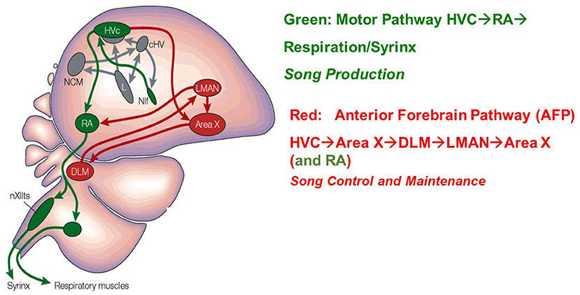
Figure 2. A drawing of the Song Production Pathway and the Anterior Forebrain Pathway of avian songbirds. Parts of the auditory pathways are shown in gray. Pathways from the brainstem that ultimately return to HVC are not shown. The HVC network image is taken from Brainard and Doupe [33]. Reprinted by permission from Copyright Clearance Center: Springer Nature.

In vitro observations of each HVC cell type have been obtained through patch-clamp techniques making intracellular voltage measurements in a reduced, brain slice preparation [23]. In this configuration, the electrode can simultaneously inject current into the neuron while measuring the whole cell voltage response [34]. From these data, one can establish the physical parameters of the system [23]. Traditionally this is done using neurochemicals to block selected ion channels and measuring the response properties of others [35]. Single current behavior is recorded and parameters are found through mathematical fits of the data. This procedure has its drawbacks, of course. There are various technical problems with the choice of channel blockers. Many of even the modern channel blockers are not subtype specific [36] and may only partially block channels [37]. A deeper conceptual problem is that is difficult to know what channels one may have missed altogether. Perhaps there are channels which express themselves only outside the bounds of the experimental conditions.

Our solution to such problems is the utilization of statistical data assimilation (SDA). This a method developed by meteorologists and others as computational models of increasingly large dynamical systems have been desired. Data assimilation has been described in our earlier sections.

In this paper, we focus on the song learning pathway, reporting on experiments involving the HVC_X neuron. The methods are generally applicable to the other neurons in HVC, and actually, to neurons seen as dynamical systems in general.

We start with a discussion about the neuron model. First we demonstrate the utility of our precision annealing methods through the use of twin experiments. These are numerical experiments in which “data” is generated through a known model (of HVC_X), then analyzed via precision annealing. In a twin experiment, we know everything, so we can verify the SDA method by looking at predictions after a observation window in which the model is trained, and we may also compare the estimations of unobserved state variables and parameters to the ingredients and output of the model.

Twin experiments are meant to mirror the circumstances of the real experiment. We start by taking the model that we think describes our physical system. Initial points for the state variables and parameters are chosen at random from a uniform distrubtion within the state/parameter bounds, which are used along with the model to numerically integrate forward in time. This leaves us with complete information about the system. Noise is added to a subset of the state variables to emulate the data to be collected in a lab experiment. We then perform PA on these simulated data, as if they were real data. The results of these numerical experiments can be used to inform laboratory experiments, and indeed help design them, by identifying the necessary measurements and stimulus needed to accurately electrophysiologically characterize a neuron.

The second set of SDA analyses we report on using “nudging,” as described above, to estimate some key biophysical properties of HVC_X neurons from laboratory data. This SDA procedure is applied to HVC_X neurons in two different birds. The results show that though each bird is capable of normal vocalization, their complement of ion channel strengths is apparently different. We report on a suggestive example of this, leaving a full discussion to Daou and Margoliash (in review).

In order to obtain good estimation results, we must choose a forcing or stimulus with the model in mind: the dynamical range of the neuron must be thoroughly explored. This suggests a few key properties of the stimulus:

• The current waveform of I_injected(t) must have sufficient amplitudes (±) and must be applied sufficiently long in time that it explores the full range of the neuron variation.

• The frequency content of the stimulus current must be a low enough that it does not exceed the low-pass cutoff frequency associated with the RC time constant of the neuron. This cutoff is typically in the neighborhood of 50–100 Hz.

• The current must explore all time scales expressed in the neuron's behavior.

3.2. Analysis of HVC_X Data

The model for an HVC_X neuron is substantially taken from Daou et al. [23] and described in Supplementary Data Sheet 1. We now use this model in a “twin experiment” in which PA is utilized, and then using “nudging” we present the analysis of experimental data on two Zebra Finch.

3.2.1. Twin Experiment on HVC_X Neuron Model

A twin experiment is a synthetic numerical experiment meant to mirror the conditions of a laboratory experiment. We use our mathematical model with some informed parameter choices in order to generate numerical data. Noise is added to observable variables in the model, here V(t). These data are then put through our SDA procedure to estimate parameters and unobserved states of the model. The neuron model is now calibrated or completed.

Using the parameters and the full state of the model at the end t_F of an observation window [t₀, t_F], we take a current waveform I_injected(t ≥ t_F) to drive the model neuron and predict the time course of all dynamical variables in the prediction window [t_F, …]. This validation of the model is the critical test of our SDA procedure, here PA. In a laboratory experiment we have no specific knowledge of the parameters in the model and, by definition, cannot observe the unobserved state variables; here we can do that. So, “fitting” the observed data within the observation window [t₀, t_F] is not enough, we must reproduce all states for t ≥ t_F to test our SDA methods.

We use the model laid out in the Supplementary Data Sheet 1. We assume that the neuron has a resting potential of −70 mV and set the initial values for the voltage and each gating variable accordingly. We assume that the internal calcium concentration of the cell is C_in = 0.1 μM. We use an integration time step of 0.02 ms and integrate forward in time using an adaptive Runge-Kutta method [6]. Noise is added to the voltage time course by sampling from a Gaussian distribution ${N}(0,2)$ in units of mV.

The waveform of the injected current was chosen to have three key attributes: (1) It is strong enough to cause spiking in the neuron, (2) it dwells a long time in a hyperpolarizing region, and (3) its overall frequency content is low enough to not be filtered out by the neuron's RC time constant. On this last point, a neuron behaves like an RC circuit, it has a cut off frequency limited by the time constant of the system. Any input current which has a frequency higher than that of the cut off frequency won't be “seen” by the neuron. The time constant is taken to be the time it takes to spike and return back to 37% above its resting voltage. We chose a current where the majority of the power spectral density exists below 50 Hz.

The first two seconds of our chosen current waveform is a varying hyperpolarizing current. In order to characterize I_h(t) and I_CaT(t), it is necessary to thoroughly explore the region where the current is active. I_h(t) is only activated when the neuron is hyperpolarized. The activation of I_h(t) deinactivates I_CaT(t), thereby allowing its dynamics to be explored. In order to characterize I_Na(t) and I_K(t), it is necessary to cause spiking in the neuron. The depolarizing current must be strong enough to hit the threshold potential for spike activation.

The parameters used to generate the data used in the twin experiment are in Table 1, and the injection current data and the membrane voltage response may be seen in Figures 3A,B.

TABLE 1

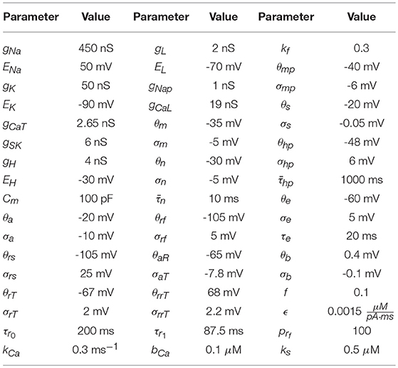
Table 1. Parameter values used to numerically generate the HVC_X data. The source of these values comes from Daou et al. [23]. Data was generated using an adaptive Runge-Kutta method, and can be seen in Figures 3A,B.

FIGURE 3

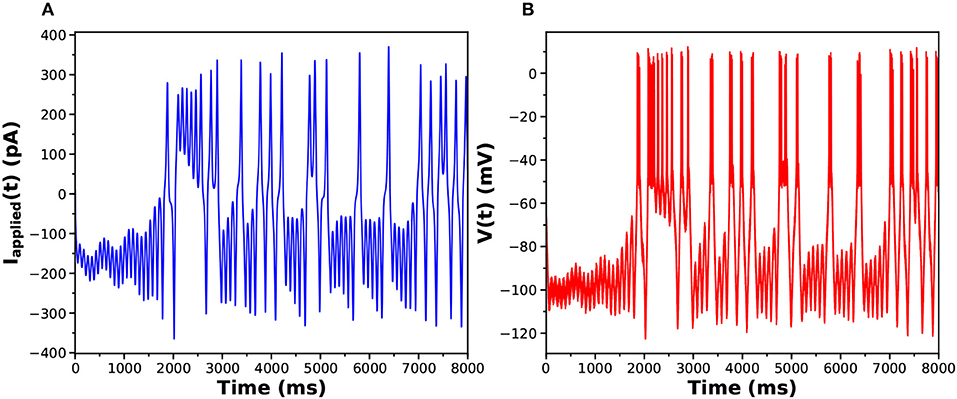
Figure 3. (A) Stimulating current I_injected(t) presented to the HVC_X model. (B) Response of the HVC_X model membrane voltage to the selected I_injected(t). The displayed time course V(t) has no added noise.

The numbers chosen for the data assimilation procedure in this paper are α = 1.4 and β ranging from 1 to 100. $R_{f,0,V}=10^{-4}$ for voltage and R_{f, 0, j} = 1 for all gating variables. These numbers are chosen because the voltage range is 100 times large than the gating variable range. Choosing a single R_{f, 0} value would result in the gating variable equations being less enforced than the voltage equation by a factor of 10⁴. The α and β numbers are chosen because we seek to make $\frac{R_f}{R_{f0}}$ sufficiently large. The α and β values chosen allow $\frac{R_f}{R_{f0}}$ to reach 10¹⁵.

During estimation we instructed our methods to estimate the inverse capacitance and estimate the ratio $g^{\prime }=\frac{g}{C_m}$ instead of g and C_m independently. That separation can present a challenge to numerical procedures. We also estimated the reversal potentials as a check on the SDA method.

Within our computational capability we can reasonably perform estimates on 50,000 data points. This captures a second of data when Δt = 0.02ms. However, there are time constants in the model neuron which are on order 1 second. In order for us to estimate the behavior of these parameters accurately, we need to see multiple instances of the full response. We need a window on the order of 2–3 s. We can obtain this by downsampling the data. We know from previous results that downsampling can lead to better estimations [38]. We take every i^th data point, depending on the level of downsampling we want to do. In this data assimilation run, we downsampled by a factor of 4 to incorporate 4 s of data in the estimation window.

We look at a plot of the action as a function of β; that is, log[R_f/R_f0]. We expect to see a leveling off of the action [16] as a function of R_f. If the action becomes independent of R_f, we can then explore how well our parameter estimations perform when integrating them forward as predictions of the calibrated model. Looking at the action plot in Figure 4, we can see there is a region in which the action appears to level off, around β = 40. It is in this region where we look for our parameter estimates.

FIGURE 4

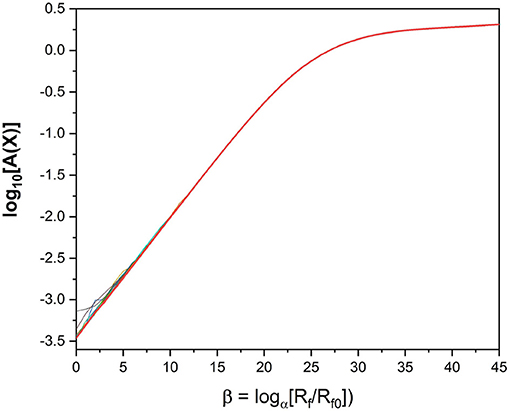
Figure 4. Action Levels of the standard model action for the HVC_X neuron model discussed in the text. We see that the action rises to a “plateau” where it becomes quite independent of R_f. The calculation of the action uses PA with α = 1.4 and R_f0 = R_m. N_I = 100 initial choices for the path X_init were used in this calculation. For small R_f one can see the slight differences in action level associated with local minima of A(X).

We examine all solutions around this region of β and utilize their parameter estimates in our predictions. We compare our numerical prediction to the “real" data from our synthetic experiment. We evaluate good predictions by finding the correlation coefficient between these two curves. This metric is chosen instead of a simple root mean square error because slight variations in spike timings yield a high amount of error even if the general spiking pattern is correct. The prediction plot and parameters for the best prediction can be seen in Figure 5 and Table 2. The voltage trace in red is the estimated voltage after data assimilation is completed. It is overlayed on the synthetic input data in black. The blue time course is a prediction, starting at the last time point of the red estimated V(t) trace and using the parameter estimates for t ≤ 4, 000ms.

TABLE 2

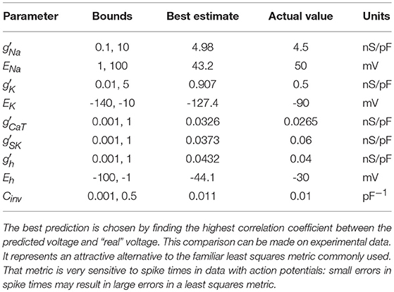
Table 2. Parameter Estimates from the Best Predictions.

FIGURE 5

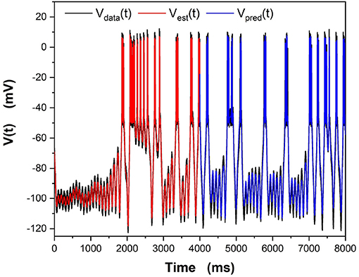
Figure 5. Results of the “twin experiment” using the model HVC_X neuron described in the Supplementary Data Sheet 1. Noise was added to data developed by solving the dynamical equations. The noisy V(t) was presented to the precision annealing SDA calculation along with the I_injected(t) in the observation window t₀ = 0ms, t_F = 4000ms. The noisy model voltage data is shown in black, and the estimated voltage is shown in red. For t ≥ 4, 000ms we show the predicted membrane voltage, in blue, generated by solving the HVC_X model equations using the parameters estimated during SDA within the observation window.

The red curve matches the computed voltage trace quite well. There is no significant deviation in the frequency of spikes, spike amplitudes, or the hyperpolarized region of the cell. Looking at the prediction window, we can see that there is some deviation in the hyperpolarized voltage trace after 7,000 ms. Our our predicted voltage does not become nearly as hyperpolarized as the real data. This is an indication that our parameter estimates for currents activated in this region are not entirely correct. Comparing parameters in Table 2, we can see that E_h is estimated as lower than its actual value. Despite that, we still are able to reproduce neuron behavior fairly well.

3.2.2. Analysis of Biophysical Parameters From HVC_X Neurons in Two Zebra Finch

Our next use of SDA employs the “nudging” method described in Eq. (9). In this section we used some of the data [Daou and Margoliash (in review)] taken in experiments on multiple HVC_X neurons from different zebra finches. The questions we asked was whether we could, using SDA, identify differences in biophysical characteristics of the birds. This question is motivated by prior biological observations [Daou and Margoliash (in review)].

Using the same HVC_X model as before, we estimated the maximal conductances {g_Na, g_K, g_CaT, g_SK, g_h} holding fixed other kinetic parameters and the Nernst/Reversal potentials. The baseline characteristics of an ion channel are set by the properties of the cell membrane and the complex proteins penetrating the membrane forming the physical channel. Differences among birds would then come from the density or numbers of various channels as characterized by the maximal conductances. If such differences were identified, it would promote further investigation of the biologically exciting proposition that these differences arise in relation to some aspect of the song learning experience of the birds [Daou and Margoliash (in review)].

In Figures 6A,B we display the stimulating current and membrane voltage response from one of 9 neurons in our large sample. The analysis using SDA was of four neurons from one bird and seven neurons from another. The results for {g_CaT, g_Na, g_SK} is displayed in Figure 7. The maximal conductances from one bird are shown in blue and from the other bird, in red. There is a striking difference between the distributions of maximal conductances.

FIGURE 6

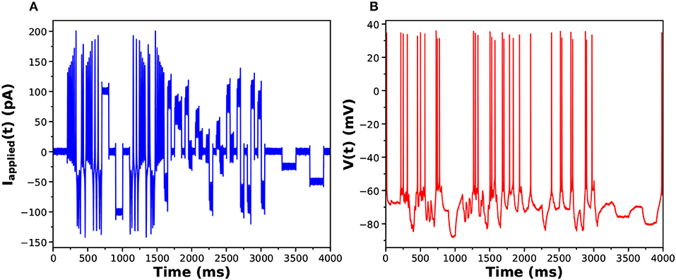
Figure 6. (A) One of the library of stimuli used in exciting voltage response activity in an HVC_X neuron. The cell was prepared in vitro, and a single patch clamp electrode injected I_injected(t) (this waveform) and recorded the membrane potential. (B) The voltage response. One of the library of stimuli used in exciting voltage response activity in an HVC_X neuron. The cell was prepared in vitro, and a single patch clamp electrode injected I_injected(t) (this waveform) and recorded the membrane potential.

FIGURE 7

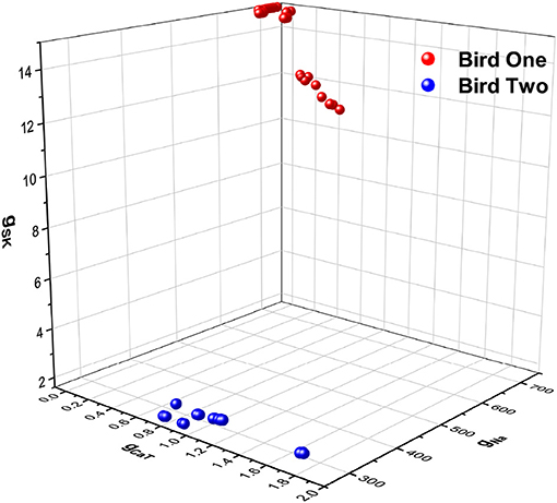
Figure 7. A three dimensional plot of three of the maximal conductances estimated from HVC_X cells using the stimulating current shown in Figure 6A. Membrane voltage responses from five neurons from one bird were recorded many times, and membrane voltage responses from four neurons from a second bird were recorded many times. One set of maximal conductances {g_Na, g_CaT, g_SK} are shown. The estimates from Bird 1 are in red-like colors, and the estimates from Bird 2 are in blue-like colors. This is just one out of a large number of examples discussed in detail in Daou and Margoliash (in review).

We do not propose here to delve into the biological implications of these results. Nevertheless, we note that the neurons from each bird occupy a small but distinct region of the parameter space (Figure 7). This result and its implications for birdsong learning, and more broadly for neuroscience, are described in Daou and Margoliash (in review). Here, however, we display this result as an example of the power of SDA to address a biologically important question in a systematic, principled manner beyond what is normally achieved in analyses of such data.

To fully embrace the utility of SDA for these experiments, however, further work is needed. A limitation of the present result is that the SDA estimates for g_SK for a subset of the neurons/observations for Bird One reach the bounds of the observation window (Figure 7). Addressing such issues would be prelude to the exciting possibility of estimating more parameters than just the principle ion currents in the Hodgkin-Huxley equations. This could use SDA numerical techniques to calculate, over hours or days, estimates of parameters that could require months or years of work to measure with traditional biological and biophysical approaches, in some cases requiring specialized equipment beyond that available for most in vitro recording set ups. In contrast, applying SDA to such data sets requires only a computer.

3.3. Analysis of Neuromorphic VLSI Instantiations of Neurons

An ambitious effort in neuroscience is the creation of low power consumption analog neural-emulating VLSI circuitry. The goals for this effort range from the challenge itself to the development of fast, reconfigurable circuitry on which to incorporate information revealed in biological experiments for use in

• creating model neural circuits of “healthy” performance to be compared to subsequent observations on the same circuitry informed by “unhealthy” performances. If the comparison can be made rapidly and accurately, the actual instantiations in the VLSI circuitry could be used to diagnose the changes in neuron properties and circuit connectivity perhaps leading to directions for cures, and

• in creating VLSI realizations of neural circuits with desired functions–say, learning syntax in interesting sequences–might allow those functions to be performed at many times increased speed than seen in the biological manifestation. If those functionalities are of engineering utility, the speed up could be critical in applications.

One of the curious roadblocks in achieving critical steps of these goals is that after the circuitry is designed and manufactured into VLSI chips, what comes back from a fabrication plant is not precisely what we designed. This is due to the realities of the manufacturing processes and not inadequacies of the designers.

To overcome this barrier in using the VLSI devices in networks, we need an algorithmic tool to determine just what did return from the factory, so we know how the nodes of a silicon network are constituted. As each chip is an electronic device built on a model design, and the flaws in manufacuring are imperfections in the realization of design parameters, we can use data from the actual chip and SDA to estimate the actual parameters on the chip.

SDA has an advantageous position here. If we present to the chip input signals with much the same design as we prepared for the neruobiological experimets discussed in the previous section, we can measure everything about each output from the chip and use SDA to estimate the actual parameters produced in manufacturing. Of course, we do not know those paramters a priori so after estimating the parameters, thus “calibrating” the chip, we must use those estimated parameters to predict the response of the chip to a new stimulating currents. That will validate (or not) the completion of the model of the actual circuitry on the chip and permit confidence in using it in building interesting networks.

We have done this on chips produced in the laboratory of Gert Cauwenberghs at UCSD using PA [38, 39] and using “nudging” as we now report.

The chip we worked with was designed to produce the simplest spiking neuron, namely one having just Na, K, and leak channels [7, 8] as in the original HH experiments. This neuron has four state variables {V(t), m(t), h(t), n(t)}:

$\begin{array}{l}C\frac{dV(t)}{dt}=g_{Na}{m}^3(t)h(t)(E_{Na}-V(t))+g_K{n}^4(t)(E_K-V(t))\\ +g_L(E_L-V(t))+I_{injected}(t)\\ \mathrm{\text{in which the gating variables }}w(t)=\left\{m(t),h(t),n(t)\right\}\mathrm{\text{ satisfy}}\\ \frac{dw(t)}{dt}=\frac{(w_{\infty }(V(t))-w(t))}{{\tau }_w(V(t))},& (13)\end{array}$

and the functions w_∞(V) are discussed in depth in Johnston and Wu [7] and Sterratt et al. [8].

In our experiments on a “NaKL” chip we used the stimulating current displayed in Figure 8,

FIGURE 8

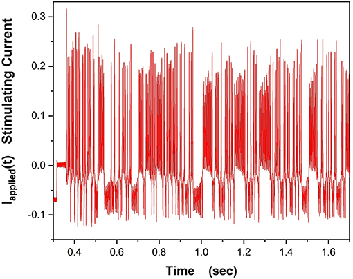
Figure 8. This waveform for I_injected(t) was used to drive the VLSI NaKL neuron after receipt from the fabrication facility.

and measured all the neural responses {V(t), m(t), h(t), n(t)}. These observations were presented to the designed model within SDA to estimate the parameters in the model.

We then tested/validated the estimations by using the calibrated model to predict how the VLSI chip would respond to a different injected current. In Figure 9 we show the observed V_data(t) in black, the estimation of the voltage through SDA in red, and the prediction of V(t) in blue for times after the end of the observation window.

FIGURE 9

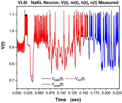
Figure 9. The NaKL VLSI neuron was driven by the waveform for I_injected(t) seen in Figure 8. The four state variables {V(t), m(t), h(t), n(t)} for the NaKL model were recorded and used in an SDA “nudging” protocol to estimate the parameters of the model actually realized at the manufacturing facility. Here we display the membrane voltages: {V_data(t), V_est(t), V_pred(t)}–the observed membrane voltage response when I_injected(t) was used, the estimated voltage response using SDA, and finally the predicted voltage response V_pred(t) from the calibrated model actually on the VLSI chip. In a laboratory experiment, only this attribute of a neuron would be observable.

While one can be pleased with the outcome of these procedures, for our purposes we see that the use of our SDA algorithms gives the user substantial confidence in the functioning characteristics of the VLSI chips one wishes to use at the nodes of a large, perhaps even very large, realization of a desired neural circuit in VLSI. We are not unaware of the software developments to allow efficient calibration of very large numbers of manufactured silicon neurons. A possible worry about also determining the connectivity, both the links and their strength and time constants, may be alleviated by realizing these links through a high bandwidth bi-directional connection of the massive array of chips and the designation of connectivity characteristics on an off-chip computer.

Part of the same analysis is the ability to observe, estimate and predict the experimentally unobservable gating variables. This serves, in this context, as a check on the SDA calculations. The Na inactivation variable h(t) is shown in Figure 10 as its measured time course h_data(t) in black, its estimated time course h_est(t) in red, and its predicted time course h_pred(t) in blue.

FIGURE 10

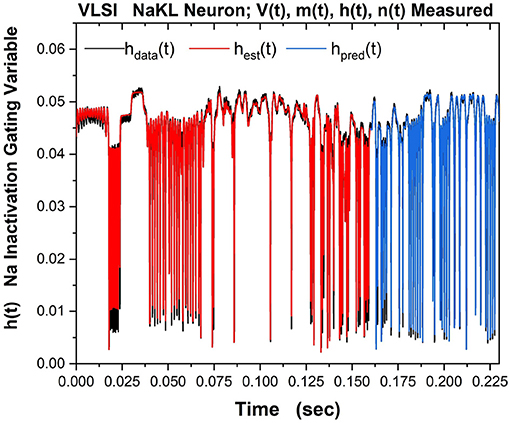
Figure 10. The NaKL VLSI neuron was driven by the waveform for I_injected(t) seen in Figure 8. The four state variables {V(t), m(t), h(t), n(t)} for the NaKL model were recorded and used in an SDA “nudging” protocol to estimate the parameters of the model actually realized at the manufacturing facility. Here we display the Na inactivation variable h(t): {h_data(t), h_est(t), h_pred(t)}–the observed h(t) time course when I_injected(t) was used, the estimated h(t) time course using SDA, and finally the predicted h(t) time course from the calibrated model actually on the VLSI chip. In a laboratory experiment, this attribute of a neuron would be unobservable. Note we have rescaled the gating variable from its natural range 0 ≤ h(t) ≤ 1) to the range within the VLSI chip. The message of this Figure is in the very good accuracy and prediction of an experimentally unobservable time course.

4. Discussion

Our review of the general formulation of statistical data assimilation (SDA) started our remarks. Many details can be found in Abarbanel [3] and subsequent papers by the authors. Recognizing that the core problem is to perform, approximately of course, the integral in Equation (6) is the essential take away message. This task requires well “curated” data and a model of the processes producing the data. In the context of experiments in life sciences or, say, aquisition of data from earth system sensors, curation includes an assessment of errors and the properties of the instruments as well.

One we have the data and a model, we still need a set of procedures to transfer the information from the data to the model, then test/validate the model on data not used to train the model. The techniques we covered are general. Their application to examples from neuroscience comprise the second part of this paper.

In the second part we first address properties of the avian songbird song production pathway and a neural control pathway modulating the learning and production of functional vocalization–song. We focus our attention on one class of neurons, HVC_X, but have also demonstrated the utility of SDA to describe the response properties of other classes of neurons in HVC, such as HVC_RA [40] and HVC_I [41]. Indeed, the SDA approach is generally applicable wherever there is insight to relate biophysical properties of neurons to their dynamics through Hodgkin Huxely equations.

Our SDA methods considered variational algorithms that seek the highest conditional probability distributions of the model states and parameters conditioned on the collection of observations over a measurement window in time. Other approaches, especially Monte Carlo algorithms were not discussed here, but are equally attractive.

We discussed methods of testing models of HVC_X neurons using “twin experiments" in which a model of the individual neuron produces synthetic data to which we add noise with a selected signal-to-noise-ratio. Some state variable time courses from the library of these model produced data, for us the voltage across the cell membrane, is then part of the action Equation (8), specifically in the measurement error term. Errors in the model are represented in the model error term of the action.

Using a precision annealing protocol to identify and track the global minimum of the action, the successful twin experiment gives us confidence in this SDA method from information trans from data to the model.

We then introduced a “nudging” method as an approximation to the Euler-Lagrange equations derived from the numerical optimization of the action Equation (8)–this is Laplace's method in our SDA context. The nudging method, introduced in meteorology some time ago, was used to distinguish between two different members of the Zebra Finch collection. We showed, in a quite preliminary manner, that the two, unrelated birds of the same species, express different HVC network properties as seen in a critical set of maximal conductances for the ion channels in their dynamics.

Finally we turned to a consideration of the challenge of implementing in VLSI technology the neurons in HVC toward the goal of building a silicon-HVC network. The challenge at the design and fabrication stages of this effort where illuminated by our use of SDA to determine what was actually returned from the manufacturing process for our analog neurons.

4.1. Moving Forward to Network Analysis

Finally, we have a few comments associated with the next stage of analysis of HVC. In this, and previous papers, we analyzed individual neurons in HVC. These analyses were assisted by our using SDA, through twin experiments, to design laboratory experiments though the selection of effective stimulilaing injected currents.

Having characterized the electrophysiology of an individual neuron within the framework of Hodgkin-Huxley (HH) models, we may now proceed beyond the study of individual neurons [42] in vitro. Once we have characterized an HVC neuron through a biophysical HH model, we may then use it in vivo as a sensor of the activity of the HVC network where it is connected to HVC_RA, HVC_I, and other HVC_X neurons. The schema for this kind of experiment is displayed in Figure 11. These experiments require the capability to perform measurements on HVC neurons in the living bird. That capability is available, and experiments as suggested in our graphic are feasible, if challenging.

FIGURE 11

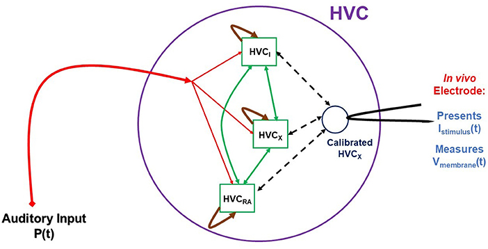
Figure 11. A cartoon-like idea of an experiment to probe the HVC network. In this graphic three neuron populations of {HVC_X, HVC_I, HVC_RA} neurons are stimulated by auditory signals P(t) presented to the bird in vivo. This drives the auditory pathway from the ear to HVC, and the network activity is recorded from a calibrated, living HVC_X neuron, used here as a sensor for network activity. While the experiment is now possible, the construction of a model HVC network will proceed in steps of complexity using simple then more biophysiclly realistic neuron models and connections among the nodes (neurons) of the network. From libraries of time courses of P(t), chosen by the user, and responses of V(t) in the “sensor” HVC_X neuron, we will use SDA to estimate properties of the network.

The schematic indicates that the stimulating input to the experiments is auditory signals, chosen by the user, presented to the bird's ear and reaching HVC through the auditory pathway. The stimuli from this signal is then distributed in a manner to be deduced from experiment and then produces activity in the HVC network that we must model. The goal is, at least initially, to establish, again within the models we develop, the connectivity of HVC neuron classes as it manifests itself in the function of the network. We have some information about this [43, 44], and these results will guide the development of the HVC model used in these whole-network experiments. An important point to address is what changes to the in vitro model might be necessary to render it a model for in vivo activity.

Data Availability

The raw data supporting the conclusions of this manuscript will be made available by the authors, without undue reservation, to any qualified researcher.

Author Contributions

AM generated and analyzed numerical data for the twin experiment on HVCX model equations. DL analyzed the biological HVCX data taken by AD. JP analyzed data from the VLSI chip. AM and HA wrote the manuscript with comments from DM, AD, JP, and DL.

Conflict of Interest Statement

The authors declare that the research was conducted in the absence of any commercial or financial relationships that could be construed as a potential conflict of interest.

Supplementary Material

The Supplementary Material for this article can be found online at: https://www.frontiersin.org/articles/10.3389/fams.2018.00053/full#supplementary-material

References

1. Lorenz EN. Predictability: a problem partly solved. In: Palmer T, Hagedorn R, editors. Predictability of Weather and Climate. Cambridge University Press, Cambridge (2006), p. 342–61.

Google Scholar

2. Evensen G. Data Assimilation: The Ensemble Kalman Filter. Berlin: Springer (2009).

Google Scholar

3. Abarbanel HDI. Predicting the Future: Completing Models of Observed Complex Systems. New York, NY: Springer (2013).

Google Scholar

4. Tong D. Statistical Physics. (2011). Available online at: www.damtp.cam.ac.uk/user/tong/statphys/sp.pdf

5. Laplace PS. Memoir of the probability of causes of events. Stat. Sci. (1986) 1:354–78. doi: 10.1214/ss/1177013621

CrossRef Full Text | Google Scholar

6. Press WH, Teukolsky SA, Vetterling WT, Flannery BP. Numerical Recipes: The Art of Scientific Computing, 3rd ed. New York, NY: Cambridge University Press (2007).

Google Scholar

7. Johnston D, Wu SMS. Foundations of Cellular Neurophysiology. Cambridge, MA: Bradford Books, MIT Press (1995).

Google Scholar

8. Sterratt D, Graham B, Gillies A, Willshaw D. Principles of Computational Modelling in Neuroscience. New York, NY: Cambridge University Press (2011).

Google Scholar

9. Abarbanel HDI, Rozdeba PJ, Shirman S. Machine learning: deepest learning as statistical data assimilation problems. Neural Comput. (2018). 30:2025–55. doi: 10.1162/neco_a_01094

PubMed Abstract | CrossRef Full Text | Google Scholar

10. Fano RM. Transmission of Information; A Statistical Theory of Communication. Cambridge, MA: MIT Press (1961).

Google Scholar

11. Kostuk M, Toth BA, Meliza CD, Margoliash D, Abarbanel HDI. Dynamical estimation of neuron and network properties II: path integral Monte Carlo methods. Biol Cybern. (2012) 106:155–67. doi: 10.1007/s00422-012-0487-5

PubMed Abstract | CrossRef Full Text | Google Scholar

12. Neal R. MCMC using hamiltonian dynamics. In: Gelman A, Jones G, Meng XL, editors. Handbook of Markov Chain Monte Carlo. Sound Parkway, NW: Chapman and Hall, CRC Press (2011). p. 113–63.

Google Scholar

13. Murty KG, Kabadi SN. Some NP-complete problems in quadratic and nonlinear programming. Math Program. (1987) 39:117–29. doi: 10.1007/BF02592948

CrossRef Full Text | Google Scholar

14. Ye J, Kadakia N, Rozdeba PJ, Abarbanel HDI, Quinn JC. Improved variational methods in statistical data assimilation. Nonlin Process Geophys. (2015) 22:205–13. doi: 10.5194/npg-22-205-2015

CrossRef Full Text | Google Scholar

15. Ye J, Rey D, Kadakia N, Eldridge M, Morone UI, Rozdeba P, et al. Systematic variational method for statistical nonlinear state and parameter estimation. Phys Rev E (2015) 92:052901. doi: 10.1103/PhysRevE.92.052901

PubMed Abstract | CrossRef Full Text | Google Scholar

16. Ye J. Systematic Annealing Approach for Statistical Data Assimilation. La Jolla, CA: University of California San Diego (2016).

Google Scholar

17. Quinn JC. A path integral approach to data assimilation in stochastic nonlinear systems. La Jolla, CA: University of California San Diego (2010).

Google Scholar

18. Shirman S. Strategic Monte Carlo and Variational Methods in Statistical Data Assimilation for Nonlinear Dynamical Systems. University of California San Diego (2018).

Google Scholar

19. Anthes R. Data assimilation and initialization of hurricane prediction models. J Atmos Sci. (1974) 31. doi: 10.1175/1520-0469(1974)031<0702:DAAIOH>2.0.CO;2

CrossRef Full Text | Google Scholar

20. Gelfand IM, Fomin SV. Calculus of Variations. Dover Publications, Inc. (1963).

Google Scholar

21. Metropolis N, Rosenbluth AW, Rosenbluth MN, Teller AH, Teller E. Equation of state calculations by fast computing machines. J Chem Phys. (1953) 21:1087–92. doi: 10.1063/1.1699114

CrossRef Full Text | Google Scholar

22. Doupe AJ, Kuhl PK. Birdsong and human speech: common themes and mechanisms. Annu. Rev. Neurosci. (1999) 22:567–631. doi: 10.1146/annurev.neuro.22.1.567

PubMed Abstract | CrossRef Full Text | Google Scholar

23. Daou A, Ross M, Johnson F, Hyson R, Bertram R. Electrophysiological characterization and computational models of HVC neurons in the zebra finch. J Neurophysiol. (2013) 110:1227–45. doi: 10.1152/jn.00162.2013

PubMed Abstract | CrossRef Full Text | Google Scholar

24. Bolhuis JJ, Okanoya K, Scarff C. Twitter evolution: converging mechanisms in birdsong and human speech. Nat Rev Neurosci. (2010) 11:747–59. doi: 10.1038/nrn2931

PubMed Abstract | CrossRef Full Text | Google Scholar

25. Fee MS, Scharff C. The songbird as a model for the generation and learning of complex sequential behaviors. ILAR J. (2010) 51:362–77. doi: 10.1093/ilar.51.4.362

PubMed Abstract | CrossRef Full Text | Google Scholar

26. Mooney R. Neuronal mechanisms for learned birdsong. Learn Mem. (2009) 16:655–69. doi: 10.1101/lm.1065209

CrossRef Full Text | Google Scholar

27. Simonyan K, Horwitz B, Jarvis E. Dopamine regulation of human speech and bird song: a critical review. Brain Lang. (2012) 122:142–50. doi: 10.1016/j.bandl.2011.12.009

PubMed Abstract | CrossRef Full Text | Google Scholar

28. Teramitsu I, Kudo LC, London SE, Geschwind DH, White SA. Parallel FoxP1 and FoxP2 expression in songbird and human brain predicts functional interaction. J Neurosci. (2004) 24:3152–63. doi: 10.1523/JNEUROSCI.5589-03.2004

PubMed Abstract | CrossRef Full Text | Google Scholar

29. Jarvis ED, Güntürkün O, Bruce L, Csillag A, Karten H, Kuenzel W, et al. Avian brains and a new understanding of vertebrate brain evolution. Nat Rev Neurosci. (2005) 6:151–9. doi: 10.1038/nrn1606

PubMed Abstract | CrossRef Full Text | Google Scholar

30. Doupe AJ, Perkel DJ, Reiner A, Stern EA. Birdbrains could teach basal ganglia research a new song. Trends Neurosci. (2005) 28:353–63. doi: 10.1016/j.tins.2005.05.005

PubMed Abstract | CrossRef Full Text | Google Scholar

31. Nottebohm F, Stokes TM, Leonard CM. Central control of song in the canary, Serinus canarius. J Compar Neurol. (1976) 165:457–86. doi: 10.1002/cne.901650405

PubMed Abstract | CrossRef Full Text | Google Scholar

32. Fortune ES, Margoliash D. Parallel pathways and convergence onto HVc and adjacent neostriatum of adult zebra finches (Taeniopygia guttata). J Compar Neurol. (1995) 360:413–41. doi: 10.1002/cne.903600305

PubMed Abstract | CrossRef Full Text | Google Scholar

33. Brainard MS, Doupe AJ. Auditory feedback in learning and maintenance of vocal behaviour. Nat Rev Neurosci. (2000) 1:31–40. doi: 10.1038/35036205

PubMed Abstract | CrossRef Full Text | Google Scholar

34. Hamill OP, Marty A, Neher E, Sakmann B, Sigworth FJ. Improved patch-clamp techniques for high-resolution current recording from cells and cell-free membrane patches. Pflügers Archiv. (1981) 391:85–100. doi: 10.1007/BF00656997

PubMed Abstract | CrossRef Full Text | Google Scholar

35. Hernández-Ochoa EO, Schneider MF. Voltage clamp methods for the study of membrane currents and SR Ca²⁺ release in adult skeletal muscle fibres. Prog Biophys Mol Biol. (2012) 108:98–118. doi: 10.1016/j.pbiomolbio.2012.01.001

CrossRef Full Text | Google Scholar

36. Bagal SK, Marron BE, Owen RM, Storer RI, Swain NA. Voltaged gated sodium channels as drug discovery targets. Channels (Austin). (2015) 9:360–6. doi: 10.1080/19336950.2015.1079674

PubMed Abstract | CrossRef Full Text | Google Scholar

37. Frolov RV, Weckström M. Harnessing the flow of excitation: TRP, voltage-gated Na(+), and voltage-gated Ca(2+) channels in contemporary medicine. In Ion Channels as Therapeutic Targets, Part A. Cambridge, MA: Academic Press (2016). p. 25–95.

PubMed Abstract | Google Scholar

38. Breen D. Characterizing Real World Neural Systems Using Variational Methods of Data Assimilation. La Jolla, CA: University of California San Diego (2017).

Google Scholar

39. Wang J, Breen D, Akinin A, Broccard F, Abarbanel HDI, Cauwenberghs G. Assimilation of biophysical neuronal dynamics in neuromorphic VLSI. Biomed Circuits Syst. (2017) 11:1258–70. doi: 10.1109/TBCAS.2017.2776198

PubMed Abstract | CrossRef Full Text | Google Scholar

40. Kadakia N, Armstrong E, Breen D, Daou A, Margoliash D, Abarbanel H. Nonlinear statistical data assimilation for HVCRA neurons in the avian song system. Biol Cybern. (2016) 110:417–34. doi: 10.1007/s00422-016-0697-3

PubMed Abstract | CrossRef Full Text | Google Scholar

41. Breen D, Shirman S, Armstrong E, Kadakia N, Abarbanel H. HVCI Neuron Properties from Statistical Data Assimilation (2016).

Google Scholar

42. Nogaret A, Meliza CD, Margoiliash D, Abarbanel. Automatic construction of predictive neuron models through large scale assimilation of electrophysiological data. Sci Rep. (2016) 6:32749. doi: 10.1038/srep32749

PubMed Abstract | CrossRef Full Text | Google Scholar

43. Mooney R, Prather JF. The HVC microcircuit: the synaptic basis for interactions between song motor and vocal plasticity pathways. J Neurosci. (2005) 25:1952–64. doi: 10.1523/JNEUROSCI.3726-04.2005

PubMed Abstract | CrossRef Full Text | Google Scholar

44. Kosche G, Vallentin D, Long MA. Interplay of inhibition and excitation shapes a premotor neural sequence. J Neurosci. (2015) 35:1217–27. doi: 10.1523/JNEUROSCI.4346-14.2015

PubMed Abstract | CrossRef Full Text | Google Scholar