A Mathematical Analysis of the Improving Sequence Effect for Monetary Rewards

1. Introduction

Generally speaking, the improving sequence effect is an anomaly revealed in the ambit of intertemporal choice by which individuals prefer sequences of outcomes, which increase over time, rather than decrease, or flat sequences with equal mean [2]. In other words, people like improvement in such a way that they would prefer to leave the best outcomes for the last maturities of the sequence [3–5]. Thus, rather than experiencing the best outcome sooner, people usually prefer to postpone a good outcome. Obviously, this is a violation of the discounted utility model [1], since individuals show a negative time preference for sequences of outcomes rather than a positive time preference, as displayed for single outcomes.

Read and Powell [6] define the improving sequence effect for monetary sequences as follows: “Given a choice between two ways of distributing a fixed amount of money over time, either as a falling sequence going from large to small, or a rising sequence going from small to large, a rational decision maker will choose a falling sequence. This is because at a non-zero rate of interest the falling sequence dominates the rising one, since any unspent money can earn interest. Despite this, there is evidence that people often prefer rising to falling sequences.”

More specifically, Loewenstein and Sicherman [7] and Loewenstein and Prelec [8] define this anomaly for income sequences in the following way: “Given a positive real rate of interest, a worker presented with alternative income sequences X = (x₁, …, x_n) and Y = (y₁, …, y_n) for otherwise identical jobs where ${\sum }_{i=1}^n{x}_i={\sum }_{i=1}^n{y}_i$, x_i > y_i, for i = 1, …, j, and y_i > x_i, for i = j + 1, …, n, should select X over Y. [… ] Sequence X dominates Y; by selecting X and saving appropriately, workers could enjoy greater consumption in every period.” However, empirical evidence shows that workers actually prefer increasing wage profiles over flat or decreasing wage profiles of greater monetary present value.

Despite this, many researchers have theoretically and empirically studied the improving sequence effect, most are cited in the following section, and none presented a mathematical analysis of this anomaly. In this way, the main contribution of this paper is the rationalization of the improving sequence effect as an anomaly, observed in the context of an intertemporal choice by using a non-separable discount function. Moreover, this manuscript finds an interesting result linking the improving sequence effect to the delay and magnitude effects.

Therefore, the main objective of this paper is to present an analysis of the improving sequence effect for monetary sequences. The organization of this paper is as follows. Section 2 provides three mathematical definitions of the improving sequence effect and the implications between them. On the other hand, section 3 includes a proof of the present value maximization principle for decreasing income sequences by using a separable discount function. Section 4 introduces the concept of a non-separable discount function to explain the improving sequence effect in the context of discrete and continuous distributions of capital. Finally, after demonstrating the relationship between the improving sequence effect and the delay and magnitude effects (section 5), section 6 summarizes and concludes the study.

2. Mathematical Definitions of the Improving Sequence Effect

Although there are several theoretical definitions of the improving sequence effect (seen in the Introduction section of this paper), to the best of our knowledge, no mathematical definitions have been proposed yet. For this reason, we provide three mathematical definitions, which support the ideas previously indicated in the Introduction section. But, before this, we have to highlight two important observations:

• Our definitions restrict the idea provided by Loewenstein and Sicherman [8] because we only consider income sequences variable in (increasing or decreasing) arithmetic progression and not general income sequences. Even a preference for a mixed response (increasing-decreasing-increasing) has been found in the case of nonmonetary outcomes [9].

• However, our third definition allows for a given income sequence to be preferred, not only over all decreasing income sequences but also over the remaining increasing income sequences.

Before discussing the three definitions of the improving sequence effect, let us introduce the following definitions from the past.

DEFINITION 1. Let R be a set of money amounts and T a set of time instants. The pair (R, T) is said to be a distribution of capital if there is a one-to-one correspondence between the elements of R and the elements of T.

In our definitions of the improving sequence effect, we will only consider a special set of money amounts, viz a sequence variable in an arithmetic progression.

DEFINITION 2. Given an amount S and a period of time n, an intertemporal choice is said to satisfy the improving sequence effect if, for every Δ > 0, the sequence

$\begin{array}{rc}(a,1),(a+\Delta ,2),(a+2\Delta ,3),\dots ,(a+(n-1)\Delta ,n),& (1)\end{array}$

where $a=\frac{S}{n}-\frac{n-1}{2}\Delta >0$, is preferred over the rest of the decreasing sequences variable in an arithmetic progression whose positive terms mature at 1, 2, …, n, all terms summing up to S.

Definition 2 can be schematically viewed in Chart 1, where the arrow +Δ_i → −Δ_j (i, j = 1, 2, 3) means that the sequence

$(a,1),(a+{\Delta }_i,2),(a+2{\Delta }_i,3),\dots ,(a+(n-1){\Delta }_i,n)$

is preferred to

$(a,1),(a-{\Delta }_j,2),(a-2{\Delta }_j,3),\dots ,(a-(n-1){\Delta }_j,n)$

both satisfying the conditions displayed in definition 2.

CHART 1

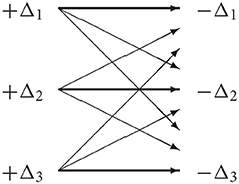
Chart 1. Scheme corresponding to Definition 2.

Definition 2, which is called the strong definition of the improving sequence effect, does not completely fit the idea underlying this anomaly since, in the empirical studies on monetary sequences [2, 4, 6, 10–14, 14], there are some decreasing sequences, which are preferred over other improving sequences, whose terms sum up to the same amount. Therefore, we provide a new definition, called the semi-strong definition of the improving sequence effect.

DEFINITION 3. Given an amount S and a period of time n, an intertemporal choice is said to satisfy the improving sequence effect if, for every Δ>0, the sequence (1) is preferred over the following decreasing sequence

$(a+(n-1)\Delta ,1),(a+(n-2)\Delta ,2),\dots ,(a+\Delta ,n-1),(a,n)$

all terms summing up to S.

Chart 2 schematizes definition 3.

CHART 2

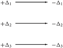
Chart 2. Scheme corresponding to Definition 3.

Despite introducing the former two definitions, the following one fits the idea of the improving sequence effect provided by Loewenstein and Sicherman [8] better. In other words, the conditions imposed on definition 2 and 3, need to be relaxed, giving rise to the weak definition of the improving sequence effect.

DEFINITION 4. Given an amount S and a period of time n, the intertemporal choice is said to satisfy the improving sequence effect if there is a Δ>0 such that sequence (1) is preferred over the rest of the sequences whose positive terms mature at 1, 2, …, n and are constant or variable (increasing or decreasing) in an arithmetic progression, all terms summing up to S.

Chart 3 schematizes definition 4.

CHART 3

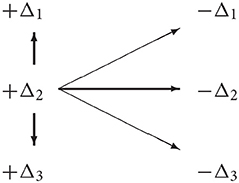
Chart 3. Scheme corresponding to Definition 4.

These three definitions fit the idea of the improving sequence effect (and the negative time preference). However, as indicated, taking into account the results obtained from the empirical studies on this effect, definition 4 fits the empirically observed behavior better than the other behaviors and also allows a computational treatment, when analytically solving the equation, leading to the preferred sequence.

PROPOSITION 1. Definition 2 implies definition 3, and definition 3 implies definition 4.

Proof. See Appendix in Supplementary Material. □

Observe that definitions 2, 3, and 4 involve all values of the common difference Δ such that the terms of the corresponding sequences are positive. However, the set of differences could be restricted to a neighborhood of zero of the form ] − k, k[, where k > 0, and incremental times to an interval [0, h], where h > 0, giving rise to the respective “local” concepts of improving sequence effect. Finally, in the rest of this paper, we only considered definitions 3 and 4.

3. Present Value Maximization Principle for Income Sequences

Loewenstein and Sicherman [7] proved through a numerical example that the present value of a decreasing sequence is greater than the present value of the constant and the improving sequences, provided that their terms total the same amount ($150,000). This statement can be generalized to mean that the present value of a sequence variable in an arithmetic progression, whose terms total a fixed amount, is decreasing with respect to the difference of the progression. This result is consistent with the financial principles: the smaller the difference, the higher the amount of the first term, which consequently is discounted using a shorter period of time than the others. Moreover, it is relevant to note that Loewenstein and Sicherman [7] used the exponential discount, which is characterized by the use of a constant instantaneous discount rate. If the instantaneous discount rate [15] is constant (exponential discounting), it is intuitive to see that the discount function cannot explain the improving sequence effect. Now, we wonder if this result can be generalized to any separable discount function, regardless of whether its instantaneous discount rate is increasing or decreasing [16]. The answer to this question is affirmative, but before that, we will introduce some formal nomenclature and notation.

Let F(t) be a (separable) discount function and let a, a+Δ, a+2Δ, …, a + (n − 1)Δ be an ordinary annuity variable in an arithmetic progression, where a > 0 is the first term and Δ is the common difference, such that the sum of all terms is constant and equal to S:

$a+(a+\Delta )+(a+2\Delta )+\cdots +\left[a+(n-1)\Delta \right]=S.$

Next, the following result can be stated.

PROPOSITION 2. The present value of the ordinary annuity whose terms are variable in arithmetic progression:

$\begin{array}{l}a,a+\Delta ,a+2\Delta ,\dots ,a+(n-1)\Delta \end{array}$

such that

$\begin{array}{l}a+(a+\Delta )+(a+2\Delta )+\cdots +\left[a+(n-1)\Delta \right]=S,\end{array}$

using any separable discount function, is decreasing with respect to Δ.

Proof. See Appendix in Supplementary Material. □

Proposition 2 can also be shown if a, a + Δ, a + 2Δ, …, a + (n − 1)Δ is an annuity due variable in arithmetic progression.

COROLLARY 1. The present value of the ordinary annuity variable in arithmetic progression

$\begin{array}{l}a,a+\Delta ,a+2\Delta ,\dots ,a+(n-1)\Delta \end{array}$

such that

$\begin{array}{l}a+(a+\Delta )+(a+2\Delta )+\cdots +\left[a+(n-1)\Delta \right]=S,\end{array}$

using the exponential discounting F(t) = (1 + i)^−t, with i > 0, is decreasing with respect to Δ. □

4. The Case of Non-Separable Discount Functions

Proposition 2 shows that, in order to explain the improving sequence effect, it is not possible to consider a separable discount function [17]. So, our first task was to define a non-separable discount function. See, for example, Lisei's paper [18].

DEFINITION 5. A non-separable discount function is a real-valued function

$F:ℝ\times {ℝ}^{+}\to ℝ$

such that

$(x,t)\mapsto F(x,t),$

satisfying the following conditions:

1. F(x, 0) = x, for every x ∈ ℝ.

2. F(0, t) = 0, for every t ∈ ℝ⁺.

3. F is increasing with respect to x. If F is differentiable, $\frac{\partial F(x,t)}{\partial x}>0$.

4. F is decreasing (respectively, increasing) with respect to t, if x > 0 (respectively, if x < 0). If F is differentiable, $\frac{\partial F(x,t)}{\partial t}<0$ (respectively, $\frac{\partial F(x,t)}{\partial t}>0)$, if x > 0 (respectively, if x < 0).

As an immediate consequence of conditions 1 and 3, it can be deduced that

$F(x,t)<x,\mathrm{\text{if}}x>0,\mathrm{\text{and}}F(x,t)>x,\mathrm{\text{if}}x<0.$

F(x, t) represents the amount at time 0, which is indifferent to the amount x at time t.

4.1. Improving Sequence Effect With Discrete Distributions of Capital

In order to verify the existence of the improving sequence effect by using a given non-separable discount function, we had to solve the following problem: to maximize the present value

$\begin{array}{l}PV={\displaystyle \sum _{t=0}^{n-1}}F(a+\Delta t,t+1).\end{array}$

This optimization problem is equivalent to solving the following equation in Δ:

$\begin{array}{l}\frac{\text{d}PV}{\text{d}\Delta }=0,\end{array}$

that is to say,

$\begin{array}{rc}{\displaystyle \sum _{t=0}^{n-1}}\left(t-\frac{n-1}{2}\right)\frac{\partial F(x,t+1)}{\partial x}{|}_{x=a+\Delta t}=0,& (2)\end{array}$

where

$\begin{array}{l}a=\frac{S}{n}-\frac{n-1}{2}\Delta .\end{array}$

Among all solutions of equation (2), we had to dismiss those such that some a + Δt (t = 0, 1, …, n − 1) was negative. Taking into account that all solutions are relative extremes, we had to choose the value of Δ corresponding to the greatest present value. To do this, if Δ₀ is a solution of equation (2), we had to verify that

$\begin{array}{rc}\frac{{\text{d}}^{2}PV}{\text{d}{\Delta }^2}{|}_{x_0=a_0+{\Delta }_{0}t}<0,& (3)\end{array}$

where

$\begin{array}{l}{a}_0=\frac{S}{n}-\frac{n-1}{2}{\Delta }_0,\end{array}$

that is to say

$\begin{array}{l}{\displaystyle \sum _{t=0}^{n-1}}{\left(t-\frac{n-1}{2}\right)}^2\frac{{\partial }^{2}F(x,t+1)}{\partial x^2}{|}_{x_0=a_0+{\Delta }_{0}t}<0.\end{array}$

EXAMPLE 1. The non-separable discount function F(x, t) = x exp{−kt/x^α}, with k > 0 and α > 1 [19], satisfies the improving sequence effect for k = 0.10, n = 3, α = 2, and S = 6. In effect, in this case,

$\begin{array}{l}\frac{\partial F(x,t)}{\partial x}=\left(1+\frac{kt\alpha }{x^{\alpha }}\right)exp\left\{-kt/x^{\alpha }\right\}\end{array}$

and

$\begin{array}{l}\frac{{\partial }^{2}F(x,t)}{\partial x^2}=\frac{kt\alpha }{x^{\alpha +1}}\left(1+\frac{kt}{x^{\alpha }}-\alpha \right)exp\left\{-kt/x^{\alpha }\right\}.\end{array}$

To solve equation (2), we obtained the value Δ₀ = 0.536. In other words, this value of Δ maximizes the present value, as represented in Figure 1. Proposition 2 proved that if the discount function depends on time t and linearly on the reward x

$F(x,t)=xF(t),$

it is not rational that the improving sequence effect can hold. In other words, the improving sequence effect can occur when the discount function depends on time and is not linear with respect to the discounted outcome

$F=F(x,t),$

as confirmed by example 1.

FIGURE 1

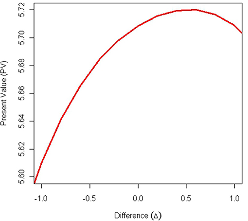
Figure 1. Present value as a function of the common difference Δ (Example 1).

Next, we wondered if alternatively this calculation could be easier if we worked with continuous distributions of capital. Before continuing with the development of the next section, we are going to introduce the following definition.

DEFINITION 6. A distribution of capital D = (R, T) is said to be continuous if T is a real interval and R(t) is a continuous function [20], where R(t)dt is the elemental amount corresponding to time t.

4.2. Improving Sequence Effect With Continuous Distributions of Capital

The objective of this subsection is to use continuous annuities for the analysis and description of the improving sequence effect. In this case, as indicated, we can not use separable discount functions. Therefore, we have to introduce the expression of the present value of a continuous annuity by using a non-separable discount function, F(x,t):

$\begin{array}{l}PV={\displaystyle \underset{n\to \infty }{lim}}{\displaystyle \sum _{k=1}^n}F\left[R(\frac{k}{n}l),\frac{k}{n}l\right]\frac{l}{n}\end{array}$

or, equivalently,

$\begin{array}{l}{\displaystyle \underset{0}{\overset{l}{\int }}}F(R(t),t)\text{d}t.\end{array}$

Obviously, in the treatment of the improving sequence effect, we will work with linear continuous annuities. More specifically, we will work with the family of continuous annuities defined by a straight line, R(t) = mt + n, such that R(t) > 0, for every t in [0, l], and where the area defined by R(t), the x-axis, and the vertical lines t = 0 and t = l is constant and equal to S. From this, there are two important remarks:

1. The slope m can be positive or negative as long as the condition R(t)>0, for every t in [0, l], holds.

2. The values of l and S are given as constants.

In this context, the expression of the present value of the continuous annuity R(t) = mt + n, valued with the non-separable discount function F(x, t), is

$\begin{array}{rc}PV={\displaystyle \underset{0}{\overset{l}{\int }}}F(mt+n,t)\text{d}t.& (4)\end{array}$

Before going further, it is necessary to show the relationship between m and n. To do this, we took the following condition into account:

$\begin{array}{l}{\displaystyle \underset{0}{\overset{l}{\int }}}(mt+n)\text{d}t=S,\end{array}$

from where

$\begin{array}{l}\left(m\frac{t^2}{2}+nt\right){|}_0^l=S,\end{array}$

or, equivalently,

$\begin{array}{l}m\frac{l^2}{2}+nl=S,\end{array}$

and finally,

$\begin{array}{l}n=\frac{S}{l}-\frac{ml}{2}.\end{array}$

Therefore,

$\begin{array}{l}R(t)=m\left(t-\frac{l}{2}\right)+\frac{S}{l}.\end{array}$

Now, we formulate the following question: Is there any value of m which maximizes the present value? If this value m₀ is positive, the improving sequence effect would hold. To do this, let us calculate the first derivative of the present value with respect to m:

$\begin{array}{l}\frac{\text{d}PV}{\text{d}m}={\displaystyle \underset{0}{\overset{l}{\int }}}\frac{\partial F(x,t)}{\partial x}{|}_{x=mt+n}\frac{\text{d}R(t)}{\text{d}m}\text{d}t.\end{array}$

Hence,

$\begin{array}{l}\frac{\text{d}R(t)}{\text{d}m}=t-\frac{l}{2}\end{array}$

and consequently

$\begin{array}{rc}\frac{\text{d}PV}{\text{d}m}={\displaystyle \underset{0}{\overset{l}{\int }}}\frac{\partial F(x,t)}{\partial x}{|}_{x=(t-\frac{l}{2})m+\frac{S}{l}}\left(t-\frac{l}{2}\right)\text{d}t.& (5)\end{array}$

Observe that, in equation (5), it is satisfied that

• $\frac{\partial F(x,t)}{\partial x}{|}_{x=(t-\frac{l}{2})m+\frac{S}{l}}>0$, by the definition of F(x, t).

• $t-\frac{l}{2}\le 0$, for every t in $\left[0,\frac{l}{2}\right]$, and $t-\frac{l}{2}\ge 0$, for every t in $\left[\frac{l}{2},l\right]$.

Therefore, the sign of the integral depends on the increase or the decrease of the factor $\frac{\partial F(x,t)}{\partial x}{|}_{x=(t-\frac{l}{2})m+\frac{S}{l}}$ with respect to t. Finally, in order to prove that the obtained value of m, denoted by m₀, is a maximum, it is necessary that

$\begin{array}{l}\frac{{\text{d}}^{2}PV}{\text{d}{m}^2}{|}_{m=m_0}<0.\end{array}$

Therefore, the use of continuous distributions of capital can facilitate the resolution of equation (2), which arises in the case of a discrete distribution of capital, and it is presented as an alternative of easy calculation.

5. Improving Sequence Effect and the Delay and Magnitude Effects

Before analyzing the relationship between the improving sequence effect and the delay and magnitude effects, the following statement can be enunciated:

PROPOSITION 3. A non-separable discount function F(x, t) describes the semi-strong improving sequence effect, for every period length h ≤ h₀, where h₀ > 0, and every amount difference −Δ₀ ≤ Δ ≤ Δ₀, with Δ₀ > 0, if and only if $\frac{{\partial }^{2}F(x,t)}{\partial x\partial t}\ge 0$ and, moreover, the set

$M:=\left\{(x,t)\in ℝ\times {ℝ}^{+}:\frac{{\partial }^{2}F(x,t)}{\partial x\partial t}>0\right\}$

is dense in the set

$N:=\left\{(x,t)\in ℝ\times {ℝ}^{+}:\frac{{\partial }^{2}F(x,t)}{\partial x\partial t}\ge 0\right\}$

in the usual topology of ℝ².

Proof. See Appendix in Supplementary Material. □

In what follows, our aim was to mathematically relate the increasing sequence effect to the delay and magnitude effects but, before this, we had to define them. Delay effect consists of using higher discount rates for short intervals than for large ones. This way, discount rates decrease as waiting time (to obtain the reward) increases.

In the experiment conducted by Benzion et al. [21], the inferred (mean) discount rates for postponing the receipt of a 200-dollar amount were 42.8, 25.5, 23.0, and 19.5% for delays of 6 months, 1, 2, and 4 years, respectively. In other words, they obtained higher average discount rates for shorter time intervals.

More specifically, Prelec and Loewenstein [22] formalized this effect in the following way: (x, t₁) ~ (y, t₂) implies (x, t₁ + h) ≺ (y, t₂ + h), for x < y and h > 0.

On the other hand, some researchers found that the rates used to discount large amounts were lower than the rates used to discount small ones, which was labeled as the magnitude effect [5]. Thaler [23] carried out an experiment where the participants were indifferent between receiving $15 right away and $60 in a year, $250 now and $350 in a year, and $3,000 immediately and $4,000 in a year, implying discount rates of 139, 34, and 29%, respectively.

This effect was expressed formally by Prelec and Loewenstein [22] as follows: (x, t₁)~(y, t₂) implies (αx, t₁)≺(αy, t₂), for α>1 and 0 < x < y (which implies t₁ < t₂). Moreover, Gerber and Rohde [24] proposed this definition: preferences exhibit the magnitude effect at date t if the outcomes x, y, X, and Y are given with 0 < x < X and 0 < y < Y, then (x, 0)~(y, t) and (X, 0)~(Y, t) implies X/Y > x/y. In the same way, Read [25] mathematically defined the magnitude effect: imagine that a small outcome $(x_1^s)$ and a large outcome $(x_1^l)$ are respectively equated with outcomes $x_2^s$ and $x_2^l$ available at different times in the future, such as $u(x_1^s)=u(x_2^s)$ and $u(x_1^l)=u(x_2^l)$, then $x_1^l/x_2^l>x_1^s/x_2^s$. However, we will use a stronger definition of the magnitude effect: (x, t₁)~(y, t₂) implies (x + k, t₁)≺(y + k, t₂), for k > 0 and 0 < x < y.

There are two behavioral explanations for this anomaly:

1. Individuals perceive and are influenced not only by relative differences but also by absolute differences in monetary amounts. The difference between $100 now and $150 in a year seems to be greater than the difference between $10 now and $15 in a year; for this reason, a lot of people are willing to wait for $50 but not for $5 [22].

2. Mental accounting [26] affects the amount entered into a mental checking. Large amounts are considered as savings and small amounts as consumption. Thus, the cost of waiting for a small reward may be perceived as a foregone consumption, whilst the opportunity cost of waiting for a large amount is perceived as a foregone interest [27].

Delay effect is equivalent to expecting that the instantaneous discount rate

$\delta (x,t)=-\frac{\frac{\partial F(x,t)}{\partial t}}{x\frac{\partial F(x,t)}{\partial x}}$

is decreasing with respect to the time t, that is to say,

$\frac{\partial \delta (x,t)}{\partial t}<0.$

Analogously, magnitude effect is equivalent to expecting that the instantaneous discount rate is decreasing with respect to the amount x, that is to say,

$\frac{\partial \delta (x,t)}{\partial x}<0.$

Once the delay and magnitude effects are characterized, the following two corollaries demonstrate that they are necessary conditions for the existence of the semi-strong improving sequence effect in terms of proposition 3.

COROLLARY 2. If a non-separable discount function F(x, t) describes the semi-strong improving sequence effect for every period length h ≤ h₀ and every amount difference −Δ₀ ≤ Δ ≤ Δ₀ and $\frac{{\partial }^{2}F(x,t)}{\partial t^2}\ge 0$, then it satisfies the delay effect.

Proof. See Appendix in Supplementary Material. □

EXAMPLE 2. Let us consider the so-called hyperbolic discount function deformed by the amount [28], that is to say, the following non-separable discount function:

$\begin{array}{l}F(x,t)=\frac{x}{1+it/x}=\frac{x^2}{x+it},\end{array}$

defined for every x ∈ ℝ⁺, where i > 0. Thus, one has

• $\frac{\partial F(x,t)}{\partial t}=-\frac{i{x}^2}{{(x+it)}^2}$.

• $\frac{\partial F(x,t)}{\partial x}=\frac{x^2+2ixt}{{(x+it)}^2}$.

Therefore, as

$\frac{{\partial }^{2}F(x,t)}{\partial t^2}=\frac{2i^2{x}^2}{{(x+it)}^3}>0$

and

$\delta (x,t)=\frac{i{x}^2}{x^3+2i{x}^{2}t}=\frac{i}{x+2it},$

F(x, t) satisfies the condition involved in the statement of corollary 2 and the delay effect (observe that δ(x, t) is strictly decreasing with respect to t).

However, as

$\frac{{\partial }^{2}F(x,t)}{\partial x\partial t}=-\frac{2i^{2}xt}{{(x+it)}^3}<0,$

F(x, t) does not satisfy the local semi-strong definition of the improving sequence effect.

COROLLARY 3. If a non-separable discount function F(x, t) describes the semi-strong improving sequence effect for every period length h ≤ h₀ and every amount difference − Δ₀ ≤ Δ ≤ Δ₀ and $\frac{{\partial }^{2}F(x,t)}{\partial x^2}\ge 0$, then it satisfies the magnitude effect.

Proof. See Appendix in Supplementary Material. □

These results fit the experimental findings from Duffy and Smith [14] who found a positive relationship between the preference for increasing payments (sequence effect) and the size of those payments (magnitude effect). Nevertheless, the converse statement of corollary 3 is not true, as shown in example 3.

EXAMPLE 3. With the same non-separable discount function of example 2, one has

$\frac{{\partial }^{2}F(x,t)}{\partial x^2}=\frac{2i^2{t}^2}{{(x+it)}^3}>0.$

Thus, F(x, t) satisfies the condition involved in the statement of corollary 3 and the magnitude effect (observe that δ(x, t) is strictly decreasing with respect to x). However, as indicated in example 2, F(x, t) does not satisfy the local semi-strong definition of the improving sequence effect.

Summarizing, under the same hypothesis of corollaries 2 and 3 some additional conditions are required in the instantaneous discount rate so that the converse statements holds. This task will be left for further research.

6. Conclusion

This paper contributes to the existing literature on the improving sequence effect by presenting a mathematical analysis of this anomaly. First of all, in order to relate this effect with other effects, we proposed three mathematical definitions of this paradox. These three definitions fit the idea of the improving sequence effect (negative time preference); however, based on the results from the empirical studies, definition 4 fits the empirically observed behavior better than the others and allows a computational treatment to find the best sequence.

Moreover, it has been mathematically proven that the present value of a sequence variable in an arithmetic progression, whose terms total a fixed amount, decreases with respect to the difference of the progression either using the exponential discount function or any other discount function. Additionally, we introduced a new methodology to detect and explain the improving sequence effect with discrete distributions of capital by using non-separable discount functions (see Example 1).

Finally, a relationship between the improving sequence effect and the delay and magnitude effects was presented. More specifically, we proved that, under certain hypotheses, the semi-strong improving sequence effect is a sufficient (but not a necessary) condition for both the delay and magnitude effects.

Author Contributions

All authors listed have made a substantial, direct and intellectual contribution to the work, and approved it for publication.

Funding

The authors gratefully acknowledge the financial support from the Spanish Ministry of Economy and Competitiveness [National R&D Project DER2016-76053-R] and from the Spanish Ministry of Economy and Science and the European Regional Development Fund-ERDF/FEDER [National R&D Project ECO2015-66504-P].

Conflict of Interest Statement

The authors declare that the research was conducted in the absence of any commercial or financial relationships that could be construed as a potential conflict of interest.

The reviewer MB and handling Editor declared their shared affiliation.

Acknowledgments

We are very grateful for the comments and suggestions offered by two referees.

Supplementary Material

The Supplementary Material for this article can be found online at: https://www.frontiersin.org/articles/10.3389/fams.2018.00055/full#supplementary-material

References

1. Samuelson PA A note on measurement of utility. Rev Econ Stud. (1937) 4:155–61. doi: 10.2307/2967612

CrossRef Full Text | Google Scholar

2. Loewenstein G, and Prelec D Preferences for sequences of outcomes. Psychol Rev. (1993) 100:91–108. doi: 10.1037/0033-295X.100.1.91

CrossRef Full Text | Google Scholar

3. Chapman GB Temporal discounting and utility for health and money. J Exp Psychol Learn Mem Cogn. (1996) 22:771–91. doi: 10.1037/0278-7393.22.3.771

PubMed Abstract | CrossRef Full Text | Google Scholar

4. Guyse J, Keller L, and Eppel T Valuing environmental outcomes: preferences for constant or improving sequences. Organ Behav Hum Decis Process. (2002) 87:253–77. doi: 10.1006/obhd.2001.2965

CrossRef Full Text | Google Scholar

5. Cruz Rambaud S, and Muñoz Torrecillas MJ An analysis of the anomalies in traditional discounting models. Int J Psychol Psychol Ther. (2004) 4:105–28.

Google Scholar

6. Read D, and Powell M Reasons for sequence preferences. J Behav Decis Making (2002) 15:433–60. doi: 10.1002/bdm.429

CrossRef Full Text | Google Scholar

7. Loewenstein G, and Sicherman N Do workers prefer increasing wage profiles? J Labor Econ. (1991) 9:67–84. doi: 10.1086/298259

CrossRef Full Text | Google Scholar

8. Loewenstein G, and Prelec D Negative time preference. Am Ec Rev. (1991) 81:347–52.

Google Scholar

9. Baucells M, Smith D, and Weber M Preferences over constructed sequences: Empirical evidence from music. Darden Business School Working Paper (2016).

Google Scholar

10. Chapman GB Expectations and preferences for sequences of health and money. Organ Behav Hum Decis Process. (1996) 67:59–75.

Google Scholar

11. Gigliotti G, and Sopher B Analysis of intertemporal choice: a new framework and experimental results. Theor Decis. (2003) 55:209–33. doi: 10.1023/B:THEO.0000044601.83386.7d

CrossRef Full Text | Google Scholar

12. Manzini P, Mariotti M, and Mittone L Choosing monetary sequences: theory and experimental evidence. Theor. Decis. (2010) 69:327–54. doi: 10.1007/s11238-010-9214-7

CrossRef Full Text | Google Scholar

13. Matsumoto D, Peecher ME, and Rich JS Evaluations of outcome sequences. Organ Behav Hum Decis Process.(2000) 83:331–52. doi: 10.1006/obhd.2000.2913

PubMed Abstract | CrossRef Full Text | Google Scholar

14. Duffy S, and Smith J Preference for increasing wages: how do people value various streams of income? Judgm Decis Making (2013) 8:74–90.

Google Scholar

15. Cruz Rambaud S, and Valls Martínez MC Introducción a las Matemáticas Financieras. 3rd ed. Madrid: Pirámide (2014).

Google Scholar

16. Cruz Rambaud S and Muñoz, Torrecillas MJ A generalization of the q-exponential discounting function. Physica A Stat Mech Appl. (2013) 392:3045–50. doi: 10.1016/j.physa.2013.03.009

CrossRef Full Text | Google Scholar

17. Musau A Hyperbolic discount curves: a reply to Ainslie. Theor Decis. (2014) 76:9–30. doi: 10.1007/s11238-013-9361-8

CrossRef Full Text | Google Scholar

18. Lisei G Su un'equazione funzionale collegata alla scindibilità delle leggi finanziarie. Giornalle dell'Istituto Italiano degli Attuari (1979) anno XLII:19–24.

Google Scholar

19. Noor J Intertemporal choice and the magnitude effect. Games Econ Behav. (2011) 72:255–70. doi: 10.1016/j.geb.2010.06.006

CrossRef Full Text | Google Scholar

20. Gil Peláez L Matemática de la Operaciones Financieras. Madrid: Editorial AC (1989).

Google Scholar

21. Benzion U, Rapaport A, and Yagil J Discount rates inferred from decisions: an experimental study. Manage Sci. (1989) 35:270–84. doi: 10.1287/mnsc.35.3.270

CrossRef Full Text | Google Scholar

22. Prelec D, and Loewenstein G Decision making over time and under uncertainty: a common approach. Manage Sci. (1991) 37:770–86. doi: 10.1287/mnsc.37.7.770

CrossRef Full Text | Google Scholar

23. Thaler R Some empirical evidence on dynamic inconsistency. Econ Lett. (1981) 1:201–7. doi: 10.1016/0165-1765(81)90067-7

CrossRef Full Text | Google Scholar

24. Gerber A, and Rohde K Anomalies in intertemporal choice? Swiss Finance Institute Research Paper. Geneva (2007).

Google Scholar

25. Read D Intertemporal choice. Working Paper LSEOR 0358. London (2003).

Google Scholar

26. Shefrin HM, and Thaler RH The behavioral life-cycle hypothesis. Econ Inquiry (1988) 26:609–43. doi: 10.1111/j.1465-7295.1988.tb01520.x

CrossRef Full Text | Google Scholar

27. Loewenstein G, and Thaler R Anomalies: intertemporal choice. J Econ Perspect. (1989) 3:181–93. doi: 10.1257/jep.3.4.181

CrossRef Full Text | Google Scholar

28. Cruz Rambaud S Parra, Oller IM and Valls Martínez MC The amount-based deformation of the q-exponential discount function: a joint analysis of delay and magnitude effects. Physica A Stat Mech Appl. (2018) 508:788–96. doi: 10.1016/j.physa.2018.05.152

CrossRef Full Text | Google Scholar