Synchronization Patterns in Modular Neuronal Networks: A Case Study of C. elegans

1. Introduction

Synchronization phenomena are widely studied across fields, from classical mechanics [1] to complex dynamical systems [2–5] and music [6, 7]. Surprising phenomena in nature, for instance, the synchronized flashing of fireflies [8] or the unexpected motion of bridges due to the emergence of synchronized walking [9] have sparked the interest in synchronization patterns. However, some more peculiar patterns of synchronization can also be observed in complex systems. These include the surprising coexistence of coherent and incoherent parts of coupled identical oscillators, a hybrid state that became known as chimera.

Chimera states were first reported in rings of non-locally and symmetrically coupled identical phase oscillators [10]. Since their discovery, they have been extensively studied both theoretically in a wide range of systems. For recent reviews see references [32–35]. For a long time, chimera states were believed to exist mostly for nonlocal coupling schemes. This consensus was revised when chimeras were found in systems of globally [36–41] and locally coupled oscillators [42–47]. Although these regular topologies often capture the nature of the interaction between the coupled elements, there are many real-world systems where a more complex connectivity description is required. Prominent examples of such systems are biological neuron networks, where synchronization is important for various cognitive functions, and chimera states, in particular, can be used to interpret phenomena such as epileptic seizures [48] and bump states [49, 50].

Previous works on the effect of nontrivial topologies on chimera states have involved scale-free and random networks [51, 52], hierarchical (fractal) schemes [53], modular structures [54], and “reflecting" connectivities [55]. Our aim is to contribute in this direction and take it one step further by considering a multilayer structure. In recent years, the study of multilayer networks has become highly popular owing to their significant relevance in several complex systems [56–58]. In the context of neuronal networks, such a multilayer approach is ideal for addressing the relationship between structure and function, an essential question in theoretical neuroscience [59]. Concerning chimera states, studies on multilayer/multiplex networks are limited and mainly deal with artificial coupling schemes [23, 60–63]. For example, the case of two populations with various coupling schemes has been systematically studied in reference [22]. In the present work, we focus on the possibility to observe chimera-like patterns in a multiplex structure of a real-world system, namely the neuronal network of Caenorhabditis elegans (C. elegans). Our main focus is to demonstrate the existence and emergence of synchronization patterns in a multilayer network obtained from the connection of this real organism. In short, we will show that chimera-like states can be hard to identify in real-world networks and suggest an alternative approach to dynamically define communities, whose dynamics can be related to biological functions to the involved neurons. The C. elegans multilayer connectome is used as a case study, but the proposed approach can be easily generalized to other networks.

The nematode C. elegans has been studied for many decades as a standard model organism for many processes of biological interest and beyond [64]. Particularly for neurobiology, the structure and connectivity of its nervous system has been deducted from reconstructions of electron micrographs of serial sections [65, 66]. Its nervous system includes sensory organs in the head and can produce highly plastic behavior, e.g., disassociative and associative learning and memory as response to taste, smell, temperature, touch and slightly to light, even though the nematode has no eyes [67]. A number of molecular mechanisms is involved in learning and memory, mediated through the same neurotransmitters as in humans and every species with a nervous system. In fact, neurons in C. elegans are very similar to those of humans, and their synapses are also classified as electrical or chemical.

It has been found that some of C. elegans' neurotransmitters, specifically the four monoamines dopamine, octopamine, serotonin and tyramine, act at both neurons and muscles to affect egg laying, pharyngeal pumping, locomotion and learning, or in general, modulate behavior in response to changing environmental cues [68]. Not only in C. elegans but also in many animals, one important route of neuromodulation is through monoamine signaling, and it is well known that this extrasynaptic communication is critical to some human brain functions. In both humans and C. elegans, many neurons expressing aminergic receptors are not post-synaptic to releasing neurons, indicating that a significant amount of monoamine signaling occurs outside the wired connectome. This defines a wireless connectivity network between neurons [69] for C. elegans. In general, this wireless or extrasynaptic communication is known as volume transmission in neuroscience [70–72], and is characterized by three-dimensional signal diffusion in the extracellular fluid, for distances larger than the synaptic cleft. This leads to multiple extracellular pathways connecting intercommunicating cells that are not well characterized from a structural perspective. For further details about our implementation of this network please refer to the Methods 5.1.

In our multilayer approach to modeling the neuronal connectivity of C. elegans, the network's nodes represent neurons connected by either electrical, chemical, or wireless pathways, which defines three layers. The electrical network is undirected, while the chemical and wireless networks are directed. Taking a closer look at the three layers' hubs in Figure 1, a strong overlap exists between hubs in the electrical and in the chemical network, however not so in the wireless network. This is in agreement with results from Bentley et al. [69], where a multilayer analysis of the three networks delineates topological overlaps between the two synaptic networks and discrepancies between the wireless and the synaptic networks. These topological differences of the different layers can be further explored by the degree distributions depicted in Figure 1, where it is clear that all of them present a heavy-tailed degree distribution with a maximum degree/average degree of 40/4 (electrical layer), 53/16 (chemical layer), and 137/15 (wireless layer). Since there are not many monoamine-releasing neurons, we observe many nodes with zero in- and out-degree. Note that the values of the wireless degree distribution need to be interpreted as maximum possible values. The underlying parameters that could lead to an equivalent of link weights are disregarded due to their complexity. Biologically, a source neuron in the wireless network influences a potential target neuron depending on parameters related to the diffusion processes of neurotransmitters throughout the body. Such parameters can be the physical distance between the presynaptic source and the postsynaptic target or the chemical concentration of the released neurotransmitters [70–72].

FIGURE 1

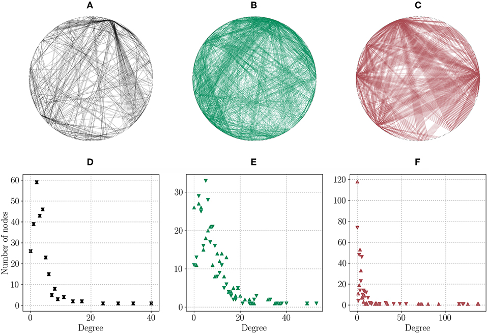
Figure 1. Layers of the C. elegans network and their degree distributions. All networks are plotted undirected and in a ring for visualization purposes only, with the same node positions across layers. ▽: in-degree, △: out-degree. (A) Electrical sub-network. (B) Chemical sub-network. (C) Wireless sub-network. (D) Electrical layer degree distribution. (E) Chemical layer in- and out-degree distribution. (F) Wireless layer in- and out-degree distribution.

In order to investigate the synchronization patterns of the neuronal network at hand, we will first investigate the dynamics based on a previous approach from Hizanidis et al. [54]. This modeling approach is then extended to get closer to the biological connectome of C. elegans. The synchronization of the network is computed based on the pairwise Euclidean distances of the dynamical variables of nodes (cf. Methods 5.3 and Kemeth et al. [73]). Furthermore, we introduce an alternative way of finding meaningful communities in the neuronal network and relate the observed synchronization patterns—including chimera-like states – to biological functions of the involved neurons.

2. Coupling by Design

Before investigating the C. elegans network using the actual connectivity data, we discuss results following the modeling approach of Hizanidis et al. [54], where first, the communities are computed from the aggregated connectome irrespective of the link type. Then, all intra-community links are assigned to the electrical layer and all inter-community links to the chemical layer. In other words, the designed network is modular or multilayer, where the neurons of each module and their intra-community links occupy a different layer. We follow this approach in order to test the applicability of the Euclidean distance method in evaluating the synchronization of the network.

Figure 2 shows the six communities obtained from the Walktrap algorithm [74] applied to the aggregated connectome of C. elegans. The resulting topology is exactly the same as in Hizanidis et al. [54]: electrical intra-community links and chemical inter-community connections. Therefore, numerical integration of the coupled Hindmarsh-Rose (Equation 1) using this topology leads to similar time series of the dynamical variable as in Hizanidis et al. [54]. See Methods 5.2 for details on the Hindmarsh-Rose model.

FIGURE 2

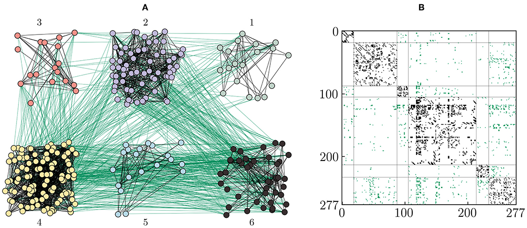
Figure 2. Topology of the artificial C. elegans network. The network of 277 neurons is divided into 6 communities of different sizes using the Walktrap algorithm. (A) Neurons are colored according to their community [1: gray (19 neurons), 2: violet (69 neurons), 3: red (18 neurons), 4: yellow (108 neurons), 5: blue (20 neurons), 6: black (43 neurons)]. Electrical and chemical connections are shown as black and green lines, respectively. In this approach, electrical junctions exist only within every communities, whereas chemical synapses span only across communities. (B) The adjacency matrix with electrical (black) and chemical (green) edges, where the axes represent the node indices. The vertical and horizontal lines divides the matrix in the ordered communities (1 to 6), from left to right in the horizontal axis, and from up to down in the vertical axis, respectively.

In Figure 3, the level of synchronization of every community γ₁ to γ₆, the global level of synchronization γ of the whole network, the chimera-like index χ_γ as well as the metastability index λ_γ are shown for a large range of electrical and chemical couplings. Note that the global level of synchronization γ is computed from the pairwise Euclidean distances of the three dimensional coordinates defined by the dynamical parameters p, q and n, between any pair of nodes in the network (cf. Methods 5.3). Thus, γ, in contrast to χ_γ and λ_γ is independent of the community structure.

FIGURE 3

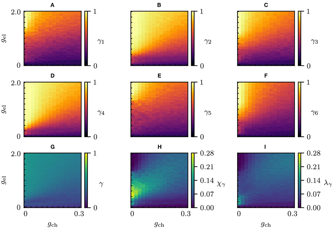
Figure 3. Synchronization parameter scans of the designed network. Changes in the community dynamical properties and global dynamical properties as the electric and chemical coupling strengths vary. (A–F) Level of synchronization of each community, γ₁ to γ₆. (G) The global level of synchronization γ of the whole network. (H) The chimera-like index χ_γ. (I) The metastability index λ_γ. System parameters: a = 1, b = 3, c = 1, d = 5, s = 4, p₀ = −1.6, I_ext = 3.25, r = 0.005, V_syn = 2 and g_wl = 0.

It can be seen that for an electrical coupling strength of g_el = 0.4 and no chemical coupling (g_ch = 0) the chimera-like index based on Euclidean distances attains a value of χ_γ ≈ 0.25. Furthermore, the metastability index for these coupling strengths λ_γ ≈ 0.12 is only half as large as the chimera-like index. This serves as justification why we may call the state a “chimera-like” state, in contrast to a “metastable” state where the metastability index prevails.

Figure 4A depicts a space-time plot of the p-variable of the Hindmarsh-Rose model, which corresponds to the membrane potential (cf. Methods 5.2) for disconnected communities with high electrical (intra-community) coupling. One can see that every community operates in the synchronized regime. For smaller electrical coupling, Figure 4B shows the space-time plot of the p-variable with a pattern of mixed synchrony that resembles a chimera-like state, that is, varying synchronization across communities. This state is achieved for g_el = 0.4 and g_ch = 0, that is, that communities are not connected. It can be seen that especially the nodes in the larger communities 2 and 4 are much more synchronized than the nodes in the small communities. The chimera-like index is still large in a close neighborhood of this point (cf. Figure 3). However, when the chemical coupling is increased, the intra-community synchronization weakens and inhibits the emergence of chimera-like states. In summary, different levels of synchronization can be achieved by means of reducing the inter-community coupling strength. This raises to the hypothesis that, when observing the designed model, the main driver of chimera-like behavior is in fact the relative size of the communities, since larger communities do not need a high intra-community coupling strength to reach a high level of synchronization. Figure 4C shows the mean order parameter depending on the size of the community. As expected, the order parameter grows with the number of nodes in the community. While the mean order parameter of the three small communities (1, 3, and 5) is always below 0.6, the largest community reaches a value of γ₄ ≈ 0.95.

FIGURE 4

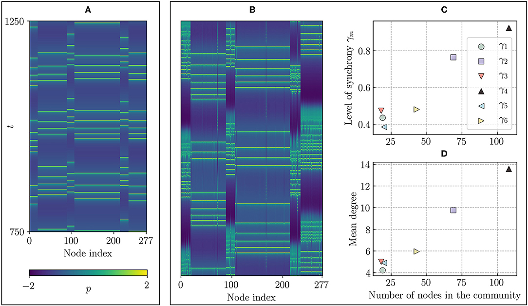
Figure 4. Space-time plots of the designed network. (A) Time series of the p-variables for a state in which every community is internally synchronized. The nodes are ordered as in Figure 2 with communities 1 to 6 from left to right. This state is achieved for g_el = 1.76, g_ch = 0. Keeping the chemical coupling at g_ch = 0 and decreasing the electrical coupling to g_el = 0.4 leads to the timeseries in panel (B), with the same color code and time scales as before, where the large communities (2 and 4) are more synchronized than the smaller communities. We call this a chimera-like state. (C) Level of synchronization γ_m and (D) mean degree of each community (m = 1, …, 6), vs. the size of the community, respectively, indicating a strong correlation between size and order. Parameters as in Figure 3.

The actual size of the community affects the order parameter only in an indirect way. What seems to be more important is the higher mean degree of nodes in the larger communities. In Figure 4D, it can be seen that there is a strong correlation between the number of nodes and the mean node degree of each community. In other words, since the nodes in large communities have more neighbors than the nodes in small communities, it is easier for them to synchronize. Note that this does not imply causality between node degree and level of synchronization. To corroborate this, more general investigations, e.g., on randomized versions of the network would be insightful. For our purpose however, it suffices to know that different community sizes influence the level of synchronization significantly.

3. Coupling by Biology

In order to investigate the synchronization of the C. elegans network even further, a third layer is added to the graph, representing the monoamine connections (wireless network). Furthermore, the assumptions about electrical and chemical synapses made in Hizanidis et al. [54] related to intra- and inter-connectivity are dropped, and the three-layer neuronal network is created using the actual connectivity data of the three synapse types (see Methods 5.1). In this section, we present two approaches to finding communities in this biological multilayer network.

3.1. Communities Based on Topology

The communities are first evaluated using a Multilayer-Louvain community detection algorithm (see Methods 5.4), which yields 8 communities instead of 6 as in the aggregated case discussed in the previous section (cf. Figure 2). Figure 5 gives an overview of the partition at hand. The adjacency matrices (Figures 5A–C) highlight clear differences between the edge types: while the wireless network, presenting few intra-community links, is distributed almost randomly across the network, the chemical layer for instance strongly reflects the underlying community structure in the adjacency matrix. Since chemical connections make up most of the edges in the network, the algorithm optimized the community partition mainly based on the chemical layer. Comparing this partition to the one in Figure 2, one can observe that the clear separation between edge types into intra- and inter-community edges is not achieved when using the biological connectome without assumptions.

FIGURE 5

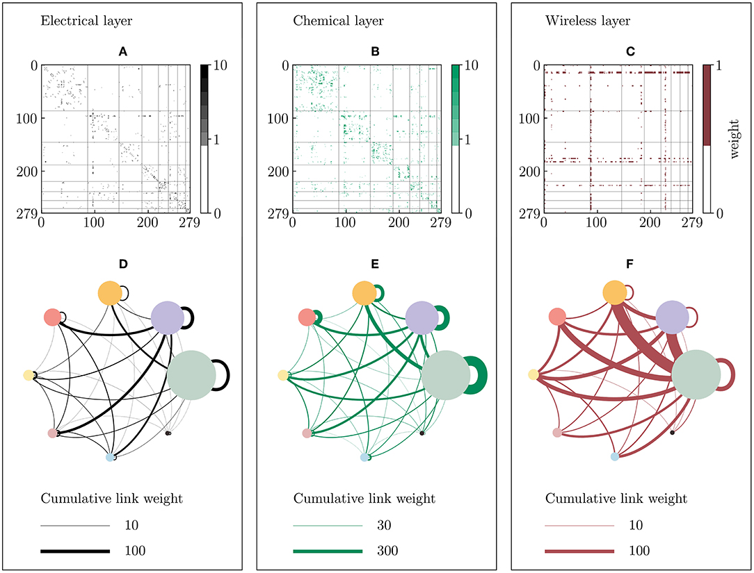
Figure 5. Communities of the Multilayer-Louvain C. elegans network. The network is divided into 8 communities of different size using the Multilayer implementation of the Louvain algorithm (see Methods 5.4). (A–C) Weighted adjacency matrices of the electrical (black), chemical (green) and wireless (red) networks, where the axes represent the node indices. The vertical and horizontal lines divides the matrix in the counter-clockwise ordered communities, from left to right in the horizontal axis, and from up to down in the vertical axis, respectively. Note that the maximum depicted weight is set to 10 in both the electrical and chemical layers for visualization reasons, even though few higher weights exist. (D–F) Inter- and intra-community coupling of the three layers, where colored circles represent communities [1: gray (87 neurons), 2: violet (59 neurons), 3: orange (43 neurons), 4: red (31 neurons), 5: yellow (19 neurons), 6: pink (17 neurons), 7: blue (15 neurons), 8: black (8 neurons)], and lines represent the cumulative link weight between two or within one community (self-loops).

The unclear separation of edge types in the partition shows its effects when analyzing the dynamics of the system using the Hindmarsh-Rose equations (see Methods 5.2). Figure 6 shows the parameter scans for the global level of synchronization γ, the chimera-like index χ_γ and the metastability index λ_γ for two different wireless coupling strengths. For the level of synchronization γ₁ to γ₈ within the individual communities (see Figures S1, S2). First of all, the global level of synchronization of the system is highly reduced when using the real connectome, which can be explained by the previously mentioned edge distribution. Since the electrical layer synchronized the nodes within communities in the designed partition, the inter-community coupling could easily be tuned using the chemical coupling strength. Therefore, a clear chimera-like region could be observed in the parameter scans in Figure 3. In the case of the real connectome, it is not possible to tune intra- and intercommunity coupling separately, since all edge types are distributed across and within communities.

FIGURE 6

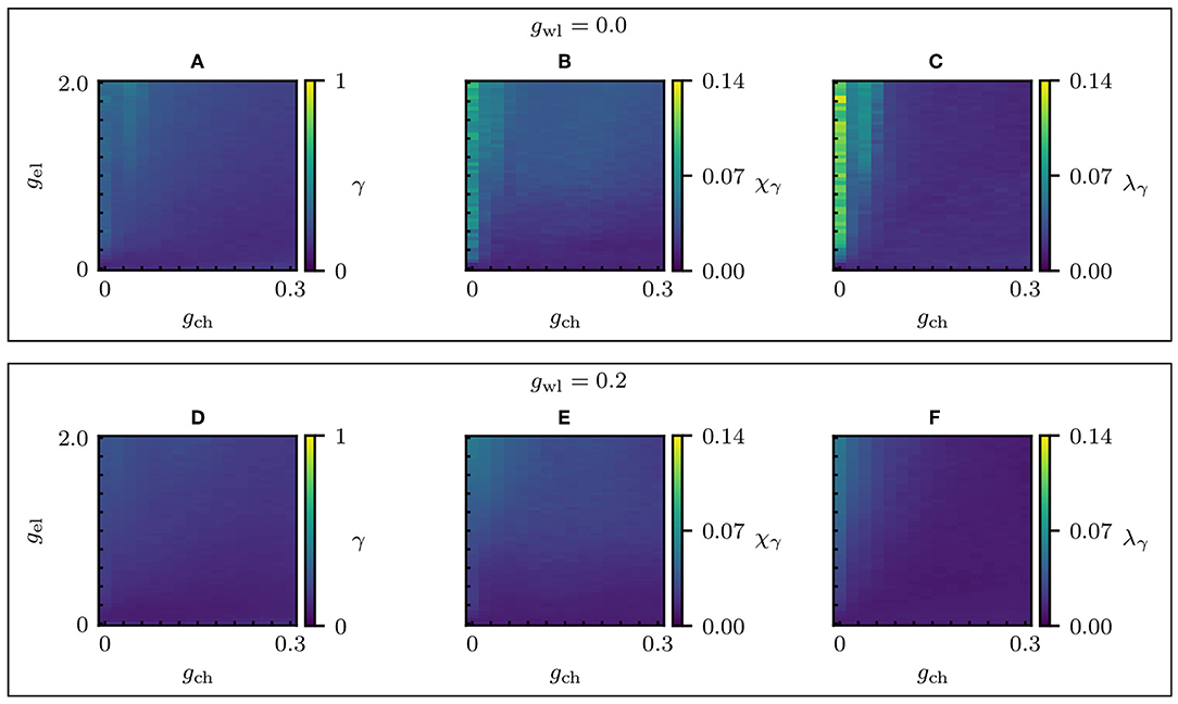
Figure 6. Synchronization parameter scans of the Multilayer-Louvain network. Changes in the global dynamical properties as the electric and chemical coupling strengths vary. (A–C) Absence of wireless coupling (g_wl = 0) for different electrical and chemical couplings: the global level of synchronization of the whole network γ, the chimera-like index χ_γ and the metastability index λ_γ. (D–F) γ, χ_γ, and λ_γ for g_wl = 0.2. The system parameters are the same as in Figure 3, except for g_wl.

Even though the parameters used to identify chimera-like states (γ, χ_γ, and λ_γ) are significantly lower than in the model by design, the timeseries of the neuron membrane potential p in Figure 7 suggest that the system adopts three different synchronization patterns, depending on the dynamical coupling strengths g_wl, g_el and g_ch. The corresponding coupling strengths and synchronization parameters are noted in Table 1. Figures 7A–C show the evolution of p for g_wl = 0.0, and Figures 7D–F show p for g_wl = 0.2. One observes that for high electrical coupling strengths (Figures 7A,D), the system is synchronized, meaning that most of the nodes follow the same periods of bursting (green) and quiescent (blue) states. However, one can see singular nodes that fall out of the synchronized pattern (especially in communities 1 to 3), which correspond to the nodes that are not electrically coupled. Figures 7C,F depict the system in the desynchronized regime, where one cannot distinguish any clear pattern of synchronization. The desynchronization becomes higher when the wireless coupling strength is increased. In Figure 7B, the system seems to exhibit chimera-like behavior at first glance. However, the chimera-like index for this coupling parameter set is very small (see Table 1). Even though community 3 seems less synchronized, one can read from the synchronization parameters (cf. Figure S1) that in fact all communities present very low synchronization. This behavior does not change significantly when adding wireless coupling (cf. Figure 7E).

FIGURE 7

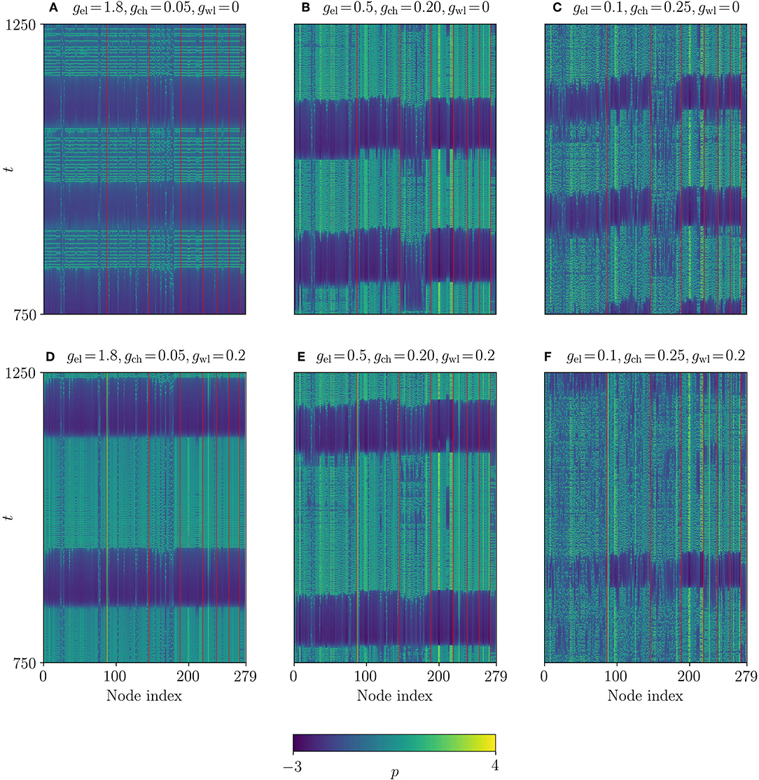
Figure 7. Space-time plots of the Multilayer-Louvain network. The system parameters are the same as in Figure 3, except for g_wl. (A–C) Temporal evolution of the p-variable for different g_el and g_ch with g_wl = 0. (D–F) Similar plots for g_wl = 0.2. The values of all coupling strengths are summarized in Table 1. Red lines separate different communities.

TABLE 1

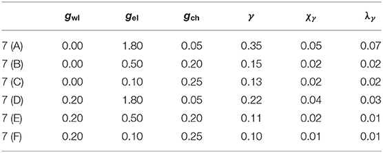
Table 1. Parameter sets used in Figure 7.

Using the Multilayer-Louvain community detection approach to partition the network, one observes a system expressing different synchronization patterns depending on the interplay of the coupling strengths of the three layers. However, even though these patterns are visible in the evolution of the p-variable (Figure 7), the topological community partition cannot reflect these patterns in the parameter scans (Figure 6). Therefore, the question about the meaning of community detection can be raised. The following section proposes an alternative way of detecting communities in multilayer networks, which is not based on the topology or link distribution, but on the correlation of nodes with respect to their dynamic variable p.

3.2. Communities Based on Dynamics

In the previous section it was shown that the Multilayer-Louvain partition already leads to significant differences in the synchronization behavior of the distinct communities. Yet, as this barely becomes apparent in the chimera-like index, we investigated an alternative approach of finding communities, based on dynamical correlations between the time series of the p-variable. The heuristic algorithm leading to the correlation-based partition is described in detail in Methods 5.5. It is worth mentioning that this algorithm only changes the partition of the network, it does not change the nodes' dynamics when compared to section 3.1, as the underlying graph itself remains untouched. However, the synchronization measures (i.e. γ_m, χ_γ, and λ_γ, see Methods 5.3) do intrinsically depend on the particular partition.

Figure 8 shows that the correlation-based partition strongly differs from the partition found with the Multilayer-Louvain algorithm. The most striking difference is the stronger heterogeneity among inter-community links in the correlation-based partition. The outgoing and incoming links between communities are relatively evenly distributed in the topology-based Multilayer-Louvain partition. In the correlation-based partition however, the two largest communities (3 and 6) are much stronger connected than the rest of the network. Furthermore, it can be seen that the two smallest communities (5 and 8) present no electrical connection to any other community in the network. In general, the electrical sub-network shows only very few inter-community links compared to the strong intra-community coupling (self-loops) of the two largest communities (3 and 6).

FIGURE 8

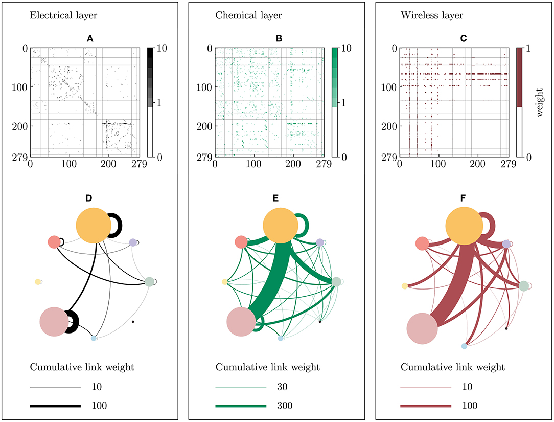
Figure 8. Communities of the dynamical correlation-based C. elegans network. The network is divided into 8 communities of different size using the correlation matrices of the p-variable from the dynamical equations (see Methods 5.5). (A–C) Weighted adjacency matrices of the electrical (black), chemical (green) and wireless (red) sub-network, where the axes represent the nodes indices. The vertical and horizontal lines divides the matrix in the counter-clockwise ordered communities, from left to right in the horizontal axis, and from up to down in the vertical axis, respectively. Note that the maximum depicted weight is set to 10 in both the electrical and chemical layers for visualization reasons, even though few higher weights exist. (D–F) Inter- and intra-community coupling of the three layers, where colored circles represent communities [1: gray (25 neurons), 2: violet (20 neurons), 3: orange (91 neurons), 4: red (33 neurons), 5: yellow (15 neurons), 6: pink (75 neurons), 7: blue (14), 8: black (6 neurons)]. Electrical and chemical connections are shown as black and green lines, respectively. Wireless connections are colored in red. In this partition, edges are distributed more clearly than in the partition obtained from the Multilayer-Louvain approach in Figure 5.

Regarding the dynamical properties, the dynamical correlation-based partition leads to qualitatively similar results as the Multilayer-Louvain partition. Compare Figures 6 and 9. In particular, Figure 9B clearly shows that the highest values of the chimera-like index χ_γ are still obtained for high electrical couplings and small chemical couplings. Increasing the wireless coupling as in Figure 9E reduces the value of χ_γ, similar to what has been observed previously in the dynamical analysis of the Multilayer-Louvain partition. However, the value of the highest chimera-like index (χ_γ ≈ 0.14, obtained at g_el = 1.96 and g_ch = 0.04) is significantly higher for the correlation-based partition. Moreover, it is also higher than the corresponding metastability index (λ_γ ≈ 0.07). Therefore, we may indeed call the state “chimera-like" [38, 54, 75–78].

FIGURE 9

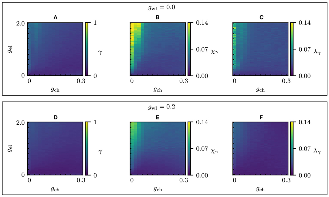
Figure 9. Synchronization parameter scans of the dynamical correlation-based network. Changes in the global dynamical properties as the electric and chemical coupling strengths vary. (A–C) Absence of wireless coupling (g_wl = 0) for different electrical and chemical couplings: the global level of synchronization of the whole network γ, the chimera-like index χ_γ and the metastability index λ_γ. (D–F) γ, χ_γ, and λ_γ for g_wl = 0.2. The system parameters are the same as in Figure 3, except for g_wl. Refer to Figures S3, S4 for the parameter scans including γ_i.

The reason for the high chimera-like index can be observed in the space time plots of the p-variables in Figure 10. As was mentioned before, the dynamics of single oscillators do not depend on the partition. In order to compare the results from the correlation-based partition with the Multilayer-Louvain partition, we decided to show the time series of p using the same coupling constants as in Figure 7. The different ordering of the nodes, though, leads to a significantly higher homogeneity between nodes within one community, which is especially apparent for the largest communities (3 and 6) in Figures 10A,D. As a consequence, the respective levels of synchronization (γ₃ ≈ 0.40 and γ₆ ≈ 0.67) are higher than for the other communities, which raises the chimera-like index. The reason for this high level of synchronization is the strong intra-community coupling of the two large communities in the electrical layer, since the electrical coupling strength is the very high in parameter set (g_el = 1.80).

FIGURE 10

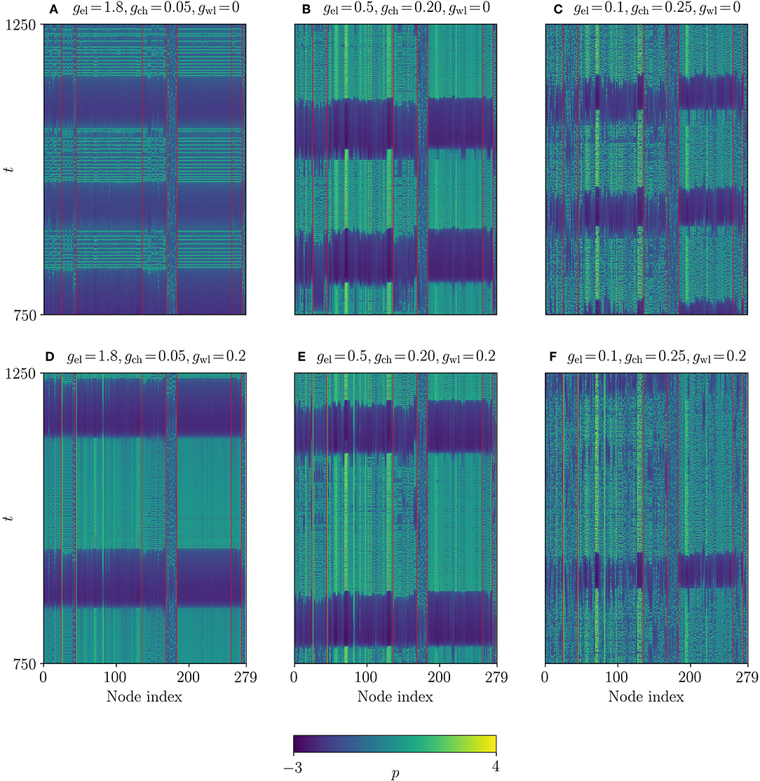
Figure 10. Space-time plots of the dynamical correlation-based network. The system parameters are the same as in Figure 3, except for g_wl. (A–C). Temporal evolution of the p-variable for different g_el and g_ch with g_wl = 0. (D–F) Similar plots for g_wl = 0.2. The values of all coupling strengths are summarized in Table 2. Red lines separate different communities. The time series are identical to Figure 7, but for a different ordering of nodes.

For time series with small electrical coupling (see Figures 10C,F), the communities are not separated as clearly, particularly when wireless coupling is applied to the system, which can be observed in Figure 10F. Especially the largest community (3) is much less synchronized, which can be explained by a stronger influence of the chemical and wireless layers, where a high number of intra-community links exist. This demonstrates that the dynamical correlation-based algorithm seems to preferentially sort the network according to the electrical sub-network, as this layer seems to be most important for the overall synchronization of the network. The adjacency matrices in Figures 8A–C support this observation: Only the electrical layer shows a large number of intra-community links, whereas the other layers present no clear visible structure. This is again in contrast to the Multilayer-Louvain partition, where the chemical layer also shows a pronounced community structure (see Figure 5B).

In the case of intermediate electrical, chemical coupling and no wireless coupling (see Figure 10B), the distinct communities can still be identified, yet the level of synchronization in the large communities does not suffice to reach a high chimera-like index. Adding wireless coupling as shown in Figure 10E does not lead to significant changes in the values.

For a full review of the different coupling strengths of to the system that lead to the time series in Figure 10, as well as the consequent values of the synchronization parameters γ, χ_γ, and λ_γ, please refer to Table 2.

TABLE 2

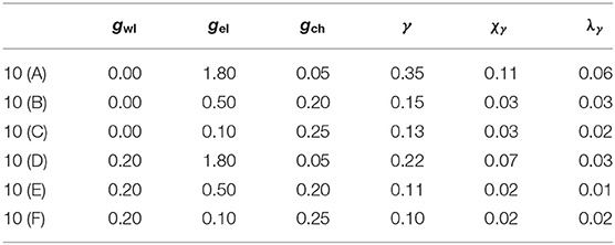
Table 2. Parameter sets used in Figure 10.

4. Discussion

Interesting synchronization patterns were found using different modeling approaches in the multilayer network of C. elegans. They were quantified based on the pairwise Euclidean distance between the dynamical variables p, q and n of the underlying Hindmarsh-Rose system (see Methods 5.3).

Following the approach of Hizanidis et al. [54], we first assume purely electrical connections within the communities, and chemical synaptic intercommunity coupling (section 2). This results in a designed coupling scenario, where chimera-like states are clearly visible due to a strong separation of connection types. While the electrical sub-network synchronizes the communities within themselves, the chemical sub-network only allows for connections across communities.

Moving toward a more biologically-inspired modeling (section 3), these synchronization states are more difficult to observe. Since the edge types are not clearly separated anymore and it is therefore impossible to tune intra- and intercommunity coupling separately, the nodes within one community cannot synchronize as easily. This is especially the case when partitioning the network with the Multilayer-Louvain algorithm: the synchronization patterns are visible in the time series (see Figure 7), but the synchronization indices are very low (see Figure 6).

We also discussed an alternative way to identify correlated clusters in the network, namely to sort nodes in communities according to the Pearson correlation matrix of the p-variable (see Methods 5.5). In this case, the community structure is dominated by two large communities with a high amount of electrical self-loops (see Figure 8) that present a strong synchronization (see Figure 10). There are two small communities that share no electrical links to the rest of the network and therefore scarcely synchronize with nodes from the other communities. This promotes the emergence of chimera-like states. Further insights on the dynamical correlation-based partition can be obtained by investigating the neuronal functions of the nodes. In Table 3, one can see that the highly synchronized communities (3 and 6) contain 75% of the motor neurons of the system. The synchronization of motor neurons under varied coupling strengths is in harmony with experimental findings, for example in rats [79].

TABLE 3

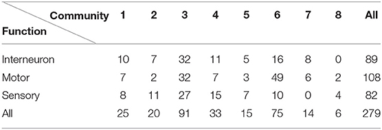
Table 3. Neuron functions of nodes in the dynamical correlation-based partition.

In this context, a question could be raised regarding the multilayer nature of the studied network. Since the three layers do not share the same number of neurons (only 253 of the 279 neurons are connected by electrical gap junctions), a certain group of nodes are prone to remain desynchronized for certain combinations of g_el, g_ch and g_wl. However, the strong biological interplay between synapse types is crucial to the understanding of the neuronal network as an entity [80, 81]. Therefore, the connectome should be modeled as a multilayer network.

Keep in mind that the studied three-layer network contains information only about the electrical, chemical and monoamine connections. Another layer could be added for the neuropeptide wireless network, which was not included since many neuropeptide receptors, as well as ligands for many neuropeptide receptors are unknown. Also, the distance over which neuropeptide signaling can occur is uncharacterized for many of them.

Furthermore, concerning the synchronization metric based on Euclidean distances (see section 5.3), the threshold parameter which defines the limit between synchronized and desynchronized nodes has been set to δ = 0.01 as in reference [73]. This value could be adapted to better suit the system and the three-dimensional distances.

This work presents an approach for analyzing the complex biological network of C. elegans using metrics of synchronization based on Euclidean distances and a new method of finding clustered nodes by correlating their dynamical variables. The underlying framework can be extended for multiple complex network applications.

5. Methods

5.1. Datasets

The gap junction and chemical synapse networks of a hermaphrodite C. elegans have been obtained in [66], and are available through WormAtlas [82]. The associated adjacency matrices are computed for the electrical and chemical layers, where we omitted the neuromuscular junctions since we are only interested in neuronal interaction. Note that this dataset does not include the 20 pharyngeal neurons. Hence, we work with the somatic giant component of the neuronal network.

The electrical sub-network consists of 253 neurons and 890 synapses or gap junctions from 517 unique neuron pairs (including 3 self-connections). A total of 352 out of 517 neuron pairs have only one synapse between them, while the other 165 pairs show multiple parallel connections, with a maximum value of 23. This means that the respective symmetric (undirected) adjacency matrix has weights varying from 1 to 23 for connected neurons.

The chemical sub-network contains 253 source and 268 target neurons, the union of both sets is composed of 279 neurons, which is the total number of nodes of the modeled C. elegans network. There are 6,294 synapses from 2,575 unique source-target neuron pairs. A total of 1,362 out of the 2,575 neuron pairs have only one synapse, while the other 1,211 pairs have multiple synaptic connections with a maximum value of 37. Therefore, the associated asymmetric (directed) adjacency matrix has weights varying from 1 to 37 for connected neurons.

The wireless sub-network of this study is restricted to the monoamine network in Bentley et al. [69] and is available in Bentley et al. [83]. Again, the pharyngeal neurons are excluded. This network by itself can be thought of as a directed quadripartite network composed of a source neuron, a neurotransmitter, a receptor and a target neuron. The considered wireless network is composed of 16 source neurons, 4 monoamine neurotransmitters, 16 associated protein receptors and 215 target neurons. As a first approach to the implementation of the wireless connectivity within our dynamical model, we are only interested in an effective connectivity between a source and a target neuron. For this purpose, we reduce the quadripartite nature by assigning binary weights to the adjacency matrix: 1, if there is any path between the neurons and 0, if there is no possible connection from a source to a target neuron through any neurotransmitter and matching receptor. The final directed adjacency matrix includes 2,282 edges.

The functional classification of the neurons in three categories (sensory, motor and interneurons) has also been obtained from [66] and manually created based on the dataset in WormAtlas [84]. We excluded the male data, since we only consider the hermaphrodite information. If the description of a particular neuron includes both interneuron and motor characteristics, we choose to describe it as motor neuron, as well as we define amphid neurons to be sensory, following the approach in Varshney et al. [66].

For details relevant to our study on the individual neurons and their characteristics, please refer to the Table S1.

5.2. Hindmarsh-Rose Dynamics

We consider a network of neurons locally characterized by Hindmarsh-Rosedynamics [85], a model intended to describe the transition between the stable resting state and the stable limit cycle of neurons. The model was intended for two types of coupling (electrical and chemical), we propose extending it by a third coupling term to account for the wireless connections in the studied network, as described by the following equations:

$\begin{array}{l}{ṗ}_i=q_i-a{p}_i^3+b{p}_i^2-n_i+I_{\text{ext}}+g_{\text{el}}{\displaystyle \sum _{j=1}^N}{L}_{ij}H(p_j)\\ -g_{\text{ch}}(p_i-V_{\text{syn}}){\displaystyle \sum _{j=1}^N}{A}_{ij}^{\text{ch}}S(p_j),-g_{\text{wl}}(p_i-V_{\text{syn}}){\displaystyle \sum _{j=1}^N}{A}_{ij}^{\text{wl}}\tilde{S}(p_j),\\ {\stackrel{\bullet }{q}}_i=c-d{p}_i^2-q_i,\\ {ṅ}_i=r\left[s(p_i-p_0)-n_i\right],& (1)\end{array}$

where i = 1, …, N is the neuron index, p_i is the membrane potential of the i-th neuron, q_i is associated with the fast current, either Na⁺ or K⁺, and n_i with the slow current, for example Ca²⁺. The parameters of Equation (1) are chosen such that a = 1, b = 3, c = 1, d = 5, s = 4, p₀ = −1.6, and I_ext = 3.25, for which the system exhibits a multi-scale chaotic behavior characterized as spike bursting [86]. The parameter r modulates the slow dynamics of the system and is set to 0.005 so that each neuron lies in the chaotic regime in the absence of coupling [54]. For these parameters, the Hindmarsh-Rosemodel enables the spike-bursting behavior of the membrane potential observed in experiments made with single neurons in vitro. We choose random initial conditions in the time series shown and find that changing the initial conditions does not change the long-term synchronization behavior. In our time series analysis, we always remove the transients and average over a long time period. The chaotic behavior of the Hindmarsh-Rosemodel has been studied in earlier publications with slightly different parameters, which led to the investigation of a plethora of chaotic phenomena using spike-counting techniques [87] and detailed bifurcation analysis [88].

The connectivity structure of the electrical synapses is described in terms of the Laplacian matrix L, whose elements are defined as $L_{ij}=A_{ij}^{\mathrm{\text{el}}}-{\delta }_{ij}{k}_i^{\mathrm{\text{el}}}$, where $k_i^{\mathrm{\text{el}}}$ is the degree of node i in the electrical layer and δ_ij = 1 if i = j, δ_ij = 0 otherwise. A^el is the symmetric adjacency matrix whose elements are $A_{ij}^{\mathrm{\text{el}}}\ne 0$ if there are electrical synapses connecting the neurons i and j, and $A_{ij}^{\mathrm{\text{el}}}=0$ otherwise. The strength of the electrical coupling is given by the parameter g_el and its functionality is governed by the linear function H(p) = p.

The connectivity structure of the chemical synapses is described by the adjacency matrix A^ch, whose elements are $A_{ij}^{\mathrm{\text{ch}}}\ne 0$ if there are chemical synapses between neurons i and j, and $A_{ij}^{\mathrm{\text{ch}}}=0$ otherwise. The nonlinear chemical coupling is described by the sigmoidal function $S(p)={\left\{1+exp\left[-{\lambda }_{\mathrm{\text{syn}}}(p-{\theta }_{\mathrm{\text{syn}}})\right]\right\}}^{-1}$, which acts as a continuous mechanism for the activation and deactivation of the chemical synapses. The associated coupling strength is noted as g_ch. For the chosen set of parameters, |p_i| < 2 and thus (p_i−V_syn) is always negative. Therefore, the chemical coupling is excitatory if V_syn = 2. The other parameters are θ_syn = −0.25 and λ_syn = 10, following references [89, 90].

The wireless connectivity structure is described by the adjacency matrix A^wl. It is also considered nonlinear; however, much slower than the chemical synaptic coupling [69]. Intuitively, the exponential function S(p) in the denominator can be decreased by replacing λ_syn with ${\tilde{\lambda }}_{\mathrm{\text{syn}}}\ll {\lambda }_{\mathrm{\text{syn}}}$. We chose ${\tilde{\lambda }}_{\mathrm{\text{syn}}}=1$, V_syn = 2 and θ_syn = −0.25, as for the chemical coupling. Furthermore, the wireless coupling is considered as an additional disrupting signal to the synchronization of the network. It is therefore treated like excitatory chemical synapses.

5.3. Level of Synchronization

We adapt an approach based on Kemeth et al. [73] in order to compute a level of synchronization of the studied network. Instead of considering the local curvature, which is optimized for a ring network, we calculate the pairwise Euclidean distances between the variables {x₁, x₂, …, x_N} at every time step t, with x_i = (p_i, q_i, n_i). For all t, we obtain a set of all possible distances between a set of N nodes:

$\begin{array}{ll}\widehat{D}\text{x}(t):=\{||{\text{x}}_i(t)-{\text{x}}_j(t)||,\forall i,j\in \{1,\dots ,N\}\}.& (2)\end{array}$

Two nodes i and j are now defined to be synchronized if ||x_i(t) − x_j(t)|| ≤ δ and desynchronized if ||x_i(t) − x_j(t)|| > δ, where δ = 0.01 · D_max is a threshold value. The value D_max is the maximum possible Euclidean distance between a pair of nodes:

$\begin{array}{ll}{D}_{\text{max}}=\sqrt{{({\text{x}}_{\text{max}}-{\text{x}}_{\text{min}})}^2},& (3)\end{array}$

where x_max = (p_max, q_max, n_max) and x_min = (p_min, q_min, n_min) are vectors containing the maximum and minimum values of the dynamical variables for all time steps t and nodes N. Therefore, two nodes are defined to be synchronized at time t if their Euclidean distance does not exceed 1% of the maximum possible distance, which is well defined for every space-time series.

Based on the set of Euclidean distances, we can measure the amount of spatially coherent nodes at each time step t. For this purpose, we consider a different set of distances, containing only those that are smaller than the threshold value δ:

$\begin{array}{ll}{\widehat{D}}_{\delta }\text{x}(t):=\{||{\text{x}}_i(t)-{\text{x}}_j(t)||<\delta ,\forall i,j\in \{1,\dots ,N\}\}.& (4)\end{array}$

The fraction between the number of distances within the range of the threshold value and the possible number of distances then results in the amount of synchronized node pairs. Note that the number of node pairs grows at a rate of N². It is therefore necessary to take the square root of this value, in order to make it comparable across network sizes. We call the resulting value “level of synchronization:”

$\begin{array}{ll}\gamma (t):=\sqrt{\frac{|{\widehat{D}}_{\delta }\text{x}(t)|}{|\widehat{D}\text{x}(t)|}}.& (5)\end{array}$

If γ(t) is only computed for a certain community m, it is called γ_m(t), representing the level of synchronization of community m at time t. For a network consisting of M communities, it is now possible to compute the chimera-like index:

$\begin{array}{ll}{\sigma }_{\gamma }(t):=\frac{1}{M-1}{\displaystyle \sum _{m=1}^M}{\left({\gamma }_m(t)-\langle {\gamma }_m(t){\rangle }_M\right)}^2& (6)\end{array}$

at time t as proposed in Shanahan [91] and also used in Hizanidis et al. [54], where 〈 γ_m(t)〉_M denotes the average level of synchronization at time t over all communities m. Thus, the only difference to Shanahan [91] is the application of the Euclidean-distance-based level of synchronization γ(t) instead of the Kuramoto order parameter. The temporal mean then defines the time-averaged chimera-like index of the network:

$\begin{array}{ll}{\tilde{\chi }}_{\gamma }:=\langle {\sigma }_{\gamma }(t){\rangle }_T.& (7)\end{array}$

Similarly we can compute the metastability index:

$\begin{array}{ll}{\sigma }_{\text{met},\gamma }(m):=\frac{1}{T-1}{\displaystyle \sum _{t=1}^T}{\left({\gamma }_m(t)-\langle {\gamma }_m(t){\rangle }_T\right)}^2& (8)\end{array}$

of community m, where 〈 γ_m(t)〉_T denotes the temporal mean of γ_m(t) over all time steps. The average over all communities yields the metastability index of the whole network:

$\begin{array}{ll}{\tilde{\lambda }}_{\gamma }=\langle {\sigma }_{\text{met},\gamma }(m){\rangle }_M.& (9)\end{array}$

The subscript γ is utilized to emphasize that these parameters differ from the parameters in Shanahan [91] and Hizanidis et al. [54] in the way the underlying level of synchronization is computed.

In order to compare community partitions with different numbers of communities, it is important to know that the ranges of χ_γ and λ_γ depend on the number of communities M of the studied network. The chimera-like index of a chimera state, where half of the communities is completely synchronized and the other half is desynchronized, becomes:

$\begin{array}{ll}{\tilde{\chi }}_{\gamma ,\text{max}}=\frac{M}{4(M-1)},& (10)\end{array}$

since the deviation from the mean is 0.5 for every community. The same considerations lead to a maximum metastability index of:

$\begin{array}{ll}{\tilde{\lambda }}_{\gamma ,\text{max}}=\frac{T}{4(T-1)},& (11)\end{array}$

which is approximately 0.25, since the total number of time steps T is large. Hence, we obtain the chimera-like and metastability indices normalized to unity:

$\begin{array}{ll}{\chi }_{\gamma }=\frac{{\tilde{\chi }}_{\gamma }}{{\tilde{\chi }}_{\gamma ,\text{max}}}& (12)\end{array}$

and,

$\begin{array}{ll}{\lambda }_{\gamma }=\frac{{\tilde{\lambda }}_{\gamma }}{{\tilde{\lambda }}_{\gamma ,\text{max}}}.& (13)\end{array}$

5.4. Multilayer-Louvain Community Detection

The communities discussed in section 3 are computed based on a multiplex Louvain community algorithm [92]. In single-layered graphs, the key to finding communities usually lies in optimizing the modularity function Q [93]:

$\begin{array}{ll}Q=\frac{1}{2m_l}{\displaystyle \sum _{i,j=1}^N}\left[A_{ij}-\frac{k_i{k}_j}{2m_l}\right]\delta (g_i,g_j),& (14)\end{array}$

where A_ij is the graph's N × N adjacency matrix, $m_l=\frac{1}{2}\sum _{i,j=1}^N{A}_{ij}$ is the total link weight in the network, and $k_i=\sum _{j=1}^N{A}_{ij}$ is the weight incident to node i. The weight of a link between i and j corresponds to the number of connections between these two nodes (see Methods 5.1). δ(g_i, g_j) = 1 if nodes i and j are in the same community, and δ(g_i, g_j) = 0 otherwise. Therefore, the term $A_{ij}-\frac{k_i{k}_j}{2m_l}$ quantifies how strongly the two nodes will be coupled in the studied network, compared to how strongly they would be coupled in a random network. In the algorithm, the function Q is computed for every pair of nodes iteratively until it reaches a maximum value.

For multilayer networks, the modularity as defined in Equation (14) is not well suited as it does not differentiate if nodes are connected by different layers. In order to extend the modularity to multilayer applications, consider a network with S layers. We define the degree of node j within the same layer as $k_j^{(\sigma )}=\sum _{i=1}^N{A}_{ij}^{(\sigma )}$, σ = 1, …, S with $A_{ij}^{(\sigma )}$ denoting the adjacency matrix in layer σ. The generalized modularity function Q_multilayer for a multilayer network with S layers is defined as [92]:

$\begin{array}{ll}{Q}_{\text{multilayer}}=\frac{1}{2\mu }{\displaystyle \sum _{i,j=1}^N}{\displaystyle \sum _{\sigma =1}^S}\left[\left(A_{ij}^{(\sigma )}-\frac{k_i^{(\sigma )}{k}_j^{(\sigma )}}{2m_{l,\sigma }}\right)\delta \left(g_i^{(\sigma )},g_j^{(\sigma )}\right)\right],& (15)\end{array}$

where $m_{l,\sigma }=\frac{1}{2}\sum _{j=1}^N{k}_j^{(\sigma )}$ is the total link weight within layer σ, and $\mu =\sum _{\sigma =1}^S{m}_{l,\sigma }$ is used for normalization similar to m_l in Equation (14). Note that in the case of the considered C. elegans network, there are no inter-layer connections, since every connection type (electrical, chemical, and wireless) represents an independent sub-network. In this study, we consider 3 layers with σ ∈ {el, ch, wl} that are shown by black, red and green link color in Figures 11A,B for the multilayer connectome and correlation-based matrix, respectively. However, Equation (15) can be extended to be used for the study of multiplex networks, in which inter-layer connections exist [92].

FIGURE 11

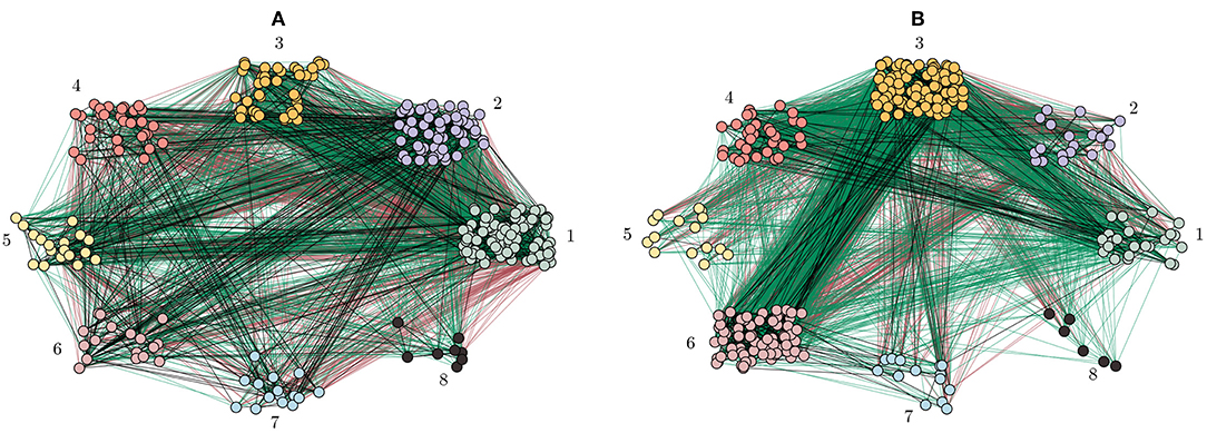
Figure 11. Community partitions of the biological C. elegans network. (A) The network is divided into 8 communities of different size using the Multilayer-Louvain algorithm (see Methods 5.4). Neurons are colored according to their community as in Figure 5. (B) The same network is partitioned using the correlation matrix approach (see Methods 5.5). Refer to Figure 8 for community sizes.

5.5. Dynamical Correlation Community Detection

We present a heuristic approach to finding meaningful communities based on the dynamics of the system. While previous approaches aimed to find a community structure based on the topology, we propose an algorithm which partitions the network based on the nodes' correlations of the p-variable.

Figure 12 shows a schematic description of the algorithm. In order to gain insight on the synchronization of the time series for each pair of nodes, we compute the Pearson-correlation matrix from the p-time series of all nodes

$\begin{array}{ll}{P}_{ij}=\frac{\langle [p_i(t)-\langle p\rangle ][p_j(t)-\langle p\rangle ]\rangle }{\sqrt{\langle p_i{(t)}^2\rangle -{\langle p\rangle }^2}\sqrt{\langle p_j{(t)}^2\rangle -{\langle p\rangle }^2}}.& (16)\end{array}$

In the hereby created matrix, every entry represents the correlation value of two time series of the two respective nodes (cf. the matrix in Figure 12, top left corner).

FIGURE 12

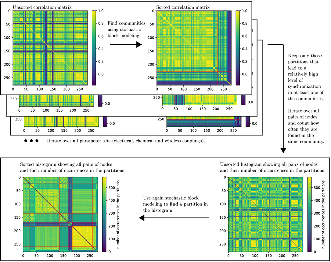
Figure 12. Schematic description of the dynamical correlation-based community detection algorithm. In the sorted matrices red lines represent the borders between two communities.

In order to find a community partition in the correlation matrix, we employ the stochastic block model approach from the graph_tool framework [94]. Since this framework does not intrinsically support weights in the network, we created a graph with a discrete number of edges between two distinct nodes that depends on the link weight in the correlation matrix; higher link weight therefore corresponds to a larger number of edges.

For every parameter set (i.e. every combination of the three different coupling strengths g_el, g_ch and g_wl) we obtain one correlation matrix, on which we apply the graph_tool algorithm. Note that, for some parameter sets, the algorithm will not find a “reasonable” partition. In particular, some partitions may consist of very small communities with only very few nodes. This is problematic in terms of the level of synchronization γ_m, since one node in a small community m plays a bigger role in the synchronization of this community; this implies stronger fluctuations of γ_m. Therefore, very small communities (especially communities consisting of only two or three nodes) can have a significantly stronger influence on the chimera-like and the metastability index than large communities. This is why we only consider community partitions with at least six nodes per community.

Another constraint applied to the partitions is a lower boundary for the level of synchronization in at least one community. The constraint is needed, because nodes do not synchronize as easily in the system based on the connectivity data (see section 3). However, a highly synchronized community is crucial to finding chimera-like states. The threshold value used to filter out partitions containing low-synchronized communities was set to γ_thr = 0.30. This is a reasonable compromise between reaching a high level of synchronization in at least one community and still keeping a relatively high number of partitions.

The algorithm finds 582 partitions that satisfy the constraints out of an initial set of 50 · 15 · 7 = 5250 possible partitions (g_el ∈ [0.04, 0.08, …, 2.00], g_ch ∈ [0.02, 0.04, …, 0.30] and g_wl ∈ [0.00, 0.05, …, 0.30]). Subsequently, we iterate over all pairs of nodes (i, j) and count how often they are found in the same community for the 582 partitions. In other words, if a pair of nodes always finds itself in the same community, the counter will be 582, while a pair that is always found in distinct communities will receive a counter of 0. This then leads to a 2-dimensional histogram as can be seen in Figure 12 in the bottom right corner.

As a final step, this histogram is sorted using the graph_tool algorithm in order to find a merged community partition that contains information over a large set of parameter values g_el, g_ch, and g_wl. The resulting sorted histogram is shown in Figure 12 in the bottom left corner and the network is visualized in Figure 11B. There is one community consisting of nodes that almost always find themselves in the same community. This implies that the time series of the corresponding nodes have a high correlation value for almost every parameter set. All the results from section 3.2 were created using this community partition.

Please note that the proposed algorithm is only one possible way of finding partitions based on a system's dynamical behavior. In fact, it invites to further explore the interplay between topology and dynamics.

Author Contributions

AP, LM, and JR had the lead analyzing the network data and performing the numerical simulations. All authors designed the study, analyzed the results, and wrote the manuscript.

Funding

AP, LM, and PH acknowledge support by Deutsche Forschungsgemeinschaft (DFG) under grant no. HO4695/3-1 and within the framework of Collaborative Research Center 910. JR acknowledges support by the German Academic Exchange Service (DAAD) and the Chilean National Commission for Scientific and Technological Research (CONICYT). NK acknowledges financial support by the MOVE-IN Louvain fellowship, co-funded by the Marie Curie Actions of the European Commission. JH acknowledges financial support by the General Secretariat for Research and Technology (GSRT) and the Hellenic Foundation for Research and Innovation (HFRI) (Code: 203).

Conflict of Interest

The authors declare that the research was conducted in the absence of any commercial or financial relationships that could be construed as a potential conflict of interest.

Acknowledgments

The authors would like to thank P. Orlowski for technical support.

Supplementary Material

The Supplementary Material for this article can be found online at: https://www.frontiersin.org/articles/10.3389/fams.2019.00052/full#supplementary-material

References

1. Ramirez JP, Olvera LA, Nijmeijer H, Alvarez J. The sympathy of two pendulum clocks: beyond Huygens' observations. Sci Rep. (2016) 6:23580. doi: 10.1038/srep23580

CrossRef Full Text | Google Scholar

2. Arenas A, Díaz-Guilera A, Kurths J, Moreno Y, Zhou C. Synchronization in complex networks. Phys Rep. (2008) 469:93–153. doi: 10.1016/j.physrep.2008.09.002

CrossRef Full Text | Google Scholar

3. Kapitaniak M, Czolczynski K, Perlikowski P, Stefanski A, Kapitaniak T. Synchronization of clocks. Phys Rep. (2012) 517:1. doi: 10.1016/j.physrep.2012.03.002

CrossRef Full Text | Google Scholar

4. Schöll E, Klapp SHL, Hövel P editors. Control of Self-organizing Nonlinear Systems. Berlin: Springer (2016).

Google Scholar

5. Boccaletti S, Pisarchik AN, del Genio CI, Amann A. Synchronization: From Coupled Systems to Complex Networks. Cambridge: Cambridge University Press (2018).

Google Scholar

6. Bader R. Nonlinearities and Synchronization in Musical Acoustics and Music Psychology. Berlin; Heidelberg: Springer (2013).

Google Scholar

7. Mukherjee S, Palit SK, Banerjee S, Ariffin MRK, Bhattacharya DK. Phase synchronization of instrumental music signals. Eur Phys J Spec Top. (2014) 223:1561–77. doi: 10.1140/epjst/e2014-02145-7

CrossRef Full Text | Google Scholar

8. Strogatz SH, Stewart I. Coupled oscillators and biological synchronization. Sci Am. (1993) 269:102–9.

PubMed Abstract | Google Scholar

9. Eckhardt B, Ott E, Strogatz SH, Abrams DM, McRobie A. Modeling walker synchronization on the Millennium Bridge. Phys Rev E. (2007) 75:021110. doi: 10.1103/PhysRevE.75.021110

PubMed Abstract | CrossRef Full Text | Google Scholar

10. Kuramoto Y, Battogtokh D. Coexistence of coherence and incoherence in nonlocally coupled phase oscillators. Nonlin Phen in Complex Sys. (2002) 5:380–5. Available online at: http://www.jp.j-npcs.org/abstracts/vol2002/v5no4/v5no4p380.html

Google Scholar

11. Abrams DM, Strogatz SH. Chimera states for coupled oscillators. Phys Rev Lett. (2004) 93:174102. doi: 10.1103/PhysRevLett.93.174102

PubMed Abstract | CrossRef Full Text | Google Scholar

12. Montbrió E, Kurths J, Blasius B. Synchronization of two interacting populations of oscillators. Phys Rev E. (2004) 70:056125. doi: 10.1103/PhysRevE.70.056125

PubMed Abstract | CrossRef Full Text | Google Scholar

13. Omel'chenko OE, Maistrenko Y, Tass P. Chimera states: the natural link between coherence and incoherence. Phys Rev Lett. (2008) 100:044105. doi: 10.1103/PhysRevLett.100.044105

PubMed Abstract | CrossRef Full Text | Google Scholar

14. Abrams DM, Mirollo RE, Strogatz SH, Wiley DA. Solvable model for chimera states of coupled oscillators. Phys Rev Lett. (2008) 101:084103. doi: 10.1103/PhysRevLett.101.084103

PubMed Abstract | CrossRef Full Text | Google Scholar

15. Pikovsky A, Rosenblum MG. Partially integrable dynamics of hierarchical populations of coupled oscillators. Phys Rev Lett. (2008) 101:264103. doi: 10.1103/PhysRevLett.101.264103

PubMed Abstract | CrossRef Full Text | Google Scholar

16. Martens EA, Laing CR, Strogatz SH. Solvable model of spiral wave chimeras. Phys Rev Lett. (2010) 104:044101. doi: 10.1103/PhysRevLett.104.044101

PubMed Abstract | CrossRef Full Text | Google Scholar

17. Martens EA. Bistable chimera attractors on a triangular network of oscillator populations. Phys Rev E. (2010) 82:016216. doi: 10.1103/PhysRevE.82.016216

PubMed Abstract | CrossRef Full Text | Google Scholar

18. Martens EA. Chimeras in a network of three oscillator populations with varying network topology. Chaos. (2010) 20:043122. doi: 10.1063/1.3499502

PubMed Abstract | CrossRef Full Text | Google Scholar

19. Omelchenko I, Maistrenko Y, Hövel P, Schöll E. Loss of coherence in dynamical networks: spatial chaos and chimera states. Phys Rev Lett. (2011) 106:234102. doi: 10.1103/PhysRevLett.106.234102

PubMed Abstract | CrossRef Full Text | Google Scholar

20. Omelchenko I, Omel'chenko OE, Hövel P, Schöll E. When nonlocal coupling between oscillators becomes stronger: patched synchrony or multichimera states. Phys Rev Lett. (2013) 110:224101. doi: 10.1103/PhysRevLett.110.224101

CrossRef Full Text | Google Scholar

21. Hizanidis J, Kanas V, Bezerianos A, Bountis T. Chimera states in networks of nonlocally coupled Hindmarsh-Rose neuron models. Int J Bifurcation Chaos. (2014) 24:1450030. doi: 10.1142/S0218127414500308

CrossRef Full Text | Google Scholar

22. Martens EA, Bick C, Panaggio MJ. Chimera states in two populations with heterogeneous phase-lag. Chaos. (2016) 26:094819. doi: 10.1063/1.4958930

PubMed Abstract | CrossRef Full Text | Google Scholar

23. Ghosh S, Zakharova A, Jalan S. Non-identical multiplexing promotes chimera states. Chaos Solitons Fractals. (2018) 106:56–60. doi: 10.1016/j.chaos.2017.11.010

CrossRef Full Text | Google Scholar

24. Calim A, Hövel P, Ozer M, Uzuntarla M. Chimera states in networks of Type-I morris-lecar neurons. Phys Rev E. (2018) 98:062217. doi: 10.1103/PhysRevE.98.062217

CrossRef Full Text | Google Scholar

25. Andrzejak RG, Ruzzene G, Malvestio I. Generalized synchronization between chimera states. Chaos. (2017) 27:053114. doi: 10.1063/1.4983841

PubMed Abstract | CrossRef Full Text | Google Scholar

26. Saha S, Bairagi N, Dana SK. Chimera states in ecological network under weighted mean-field dispersal of species. Front Appl Math Stat. (2019) 5:15. doi: 10.3389/fams.2019.00015

CrossRef Full Text | Google Scholar

27. Tinsley MR, Nkomo S, Showalter K. Chimera and phase cluster states in populations of coupled chemical oscillators. Nat Phys. (2012) 8:662–5. doi: 10.1038/nphys2371

CrossRef Full Text | Google Scholar

28. Hagerstrom AM, Murphy TE, Roy R, Hövel P, Omelchenko I, Schöll E. Experimental observation of chimeras in coupled-map lattices. Nat Phys. (2012) 8:658–61. doi: 10.1038/nphys2372

CrossRef Full Text | Google Scholar

29. Martens EA, Thutupalli S, Fourriere A, Hallatschek O. Chimera states in mechanical oscillator networks. Proc Natl Acad Sci USA. (2013) 110:10563. doi: 10.1073/pnas.1302880110

PubMed Abstract | CrossRef Full Text | Google Scholar

30. Gambuzza LV, Buscarino A, Chessari S, Fortuna L, Meucci R, Frasca M. Experimental investigation of chimera states with quiescent and synchronous domains in coupled electronic oscillators. Phys Rev E. (2014) 90:032905. doi: 10.1103/PhysRevE.90.032905

PubMed Abstract | CrossRef Full Text | Google Scholar

31. Totz J, Rode J, Tinsley MR, Showalter K, Engel H. Spiral wave chimera states in large populations of coupled chemical oscillators. Nat Phys. (2018) 14:282–5. doi: 10.1038/s41567-017-0005-8

CrossRef Full Text | Google Scholar

32. Panaggio MJ, Abrams DM. Chimera states: coexistence of coherence and incoherence in networks of coupled oscillators. Nonlinearity. (2015) 28:R67. doi: 10.1088/0951-7715/28/3/R67

CrossRef Full Text | Google Scholar

33. Schöll E. Synchronization patterns and chimera states in complex networks: interplay of topology and dynamics. Eur Phys J Spec Top. (2016) 225:891–919. doi: 10.1140/epjst/e2016-02646-3

CrossRef Full Text | Google Scholar

34. Omel'chenko OE. The mathematics behind chimera states. Nonlinearity. (2018) 31:R121. doi: 10.1088/1361-6544/aaaa07

CrossRef Full Text | Google Scholar

35. Majhi S, Bera BK, Ghosh D, Perc M. Chimera states in neuronal networks: a review. Phys Life Rev. (2019) 26:100. doi: 10.1016/j.plrev.2018.09.003

CrossRef Full Text | Google Scholar

36. Schmidt L, Schönleber K, Krischer K, García-Morales V. Coexistence of synchrony and incoherence in oscillatory media under nonlinear global coupling. Chaos. (2014) 24:013102. doi: 10.1063/1.4858996

PubMed Abstract | CrossRef Full Text | Google Scholar

37. Sethia GC, Sen A. Chimera states: the existence criteria revisited. Phys Rev Lett. (2014) 112:144101. doi: 10.1103/PhysRevLett.112.144101

PubMed Abstract | CrossRef Full Text | Google Scholar

38. Yeldesbay A, Pikovsky A, Rosenblum M. Chimeralike states in an ensemble of globally coupled oscillators. Phys Rev Lett. (2014) 112:144103. doi: 10.1103/PhysRevLett.112.144103

PubMed Abstract | CrossRef Full Text | Google Scholar

39. Böhm F, Zakharova A, Schöll E, Lüdge K. Amplitude-phase coupling drives chimera states in globally coupled laser networks. Phys Rev E. (2015) 91:040901. doi: 10.1103/PhysRevE.92.069905

PubMed Abstract | CrossRef Full Text | Google Scholar

40. Mishra A, Hens C, Bose M, Roy PK, Dana SK. Chimeralike states in a network of oscillators under attractive and repulsive global coupling. Phys Rev E. (2015) 92:062920. doi: 10.1103/PhysRevE.92.062920

PubMed Abstract | CrossRef Full Text | Google Scholar

41. Mishra A, Saha S, Hens C, Roy PK, Bose M, Louodop P, et al. Coherent libration to coherent rotational dynamics via chimeralike states and clustering in a Josephson junction array. Phys Rev E. (2017) 95:010201. doi: 10.1103/PhysRevE.95.010201

PubMed Abstract | CrossRef Full Text | Google Scholar

42. Laing CR. Chimeras in networks with purely local coupling. Phys Rev E. (2015) 92:050904. doi: 10.1103/PhysRevE.92.050904

PubMed Abstract | CrossRef Full Text | Google Scholar

43. Hizanidis J, Lazarides N, Tsironis GP. Robust chimera states in SQUID metamaterials with local interactions. Phys Rev E. (2016) 94:032219. doi: 10.1103/PhysRevE.94.032219

PubMed Abstract | CrossRef Full Text | Google Scholar

44. Bera BK, Ghosh D. Chimera states in purely local delay-coupled oscillators. Phys Rev E. (2016) 93:052223. doi: 10.1103/PhysRevE.93.052223

PubMed Abstract | CrossRef Full Text | Google Scholar

45. Clerc MG, Coulibaly S, Ferreira AM, Rojas R. Chimera states in a Duffing oscillators chain coupled to nearest neighbors. Chaos. (2018) 28:083126. doi: 10.1063/1.5025038

PubMed Abstract | CrossRef Full Text | Google Scholar

46. Bera BK, Ghosh D, Lakshmanan M. Chimera states in bursting neurons. Phys Rev E. (2016) 93:012205. doi: 10.1103/PhysRevE.93.012205

PubMed Abstract | CrossRef Full Text | Google Scholar

47. Belykh I, de Lange E, Hasler M. Synchronization of bursting neurons: what matters in the network topology. Phys Rev Lett. (2005) 94:188101. doi: 10.1103/PhysRevLett.94.188101

PubMed Abstract | CrossRef Full Text | Google Scholar

48. Andrzejak RG, Rummel C, Mormann F, Schindler K. All together now: analogies between chimera state collapses and epileptic seizures. Sci Rep. (2016) 6:23000. doi: 10.1038/srep23000

PubMed Abstract | CrossRef Full Text | Google Scholar

49. Laing CR, Chow CC. Stationary bumps in networks of spiking neurons. Neural Comput. (2001) 13:1473–94. doi: 10.1162/089976601750264974

PubMed Abstract | CrossRef Full Text | Google Scholar

50. Sakaguchi H. Instability of synchronized motion in nonlocally coupled neural oscillators. Phys Rev E. (2006) 73:031907. doi: 10.1103/PhysRevE.73.031907

PubMed Abstract | CrossRef Full Text | Google Scholar

51. Laing CR, Rajendran K, Kevrekidis YG. Chimeras in random non-complete networks of phase oscillators. Chaos. (2012) 22:043104. doi: 10.1063/1.3694118

PubMed Abstract | CrossRef Full Text | Google Scholar

52. Zhu Y, Zheng Z, Yang J. Chimera states on complex networks. Phys Rev E. (2014) 89:022914. doi: 10.1103/PhysRevE.89.022914

PubMed Abstract | CrossRef Full Text | Google Scholar

53. Omelchenko I, Provata A, Hizanidis J, Schöll E, Hövel P. Robustness of chimera states for coupled FitzHugh-Nagumo oscillators. Phys Rev E. (2015) 91:022917. doi: 10.1103/PhysRevE.91.022917

PubMed Abstract | CrossRef Full Text | Google Scholar

54. Hizanidis J, Kouvaris NE, Zamora-López G, Díaz-Guilera A, Antonopoulos C. Chimera-like states in modular neural networks. Sci Rep. (2016) 6:19845. doi: 10.1038/srep22314

CrossRef Full Text | Google Scholar

55. Tsigkri-DeSmedt ND, Hizanidis J, Schöll E, Hövel P, Provata A. Chimeras in leaky integrate-and-fire neural networks: effects of reflecting connectivities. Eur Phys J B. (2017) 90:139. doi: 10.1140/epjb/e2017-80162-0

CrossRef Full Text | Google Scholar

56. De Domenico M, Solé-Ribalta A, Cozzo E, Kivelä M, Moreno Y, Porter MA, et al. Mathematical formulation of multilayer networks. Phys Rev X. (2013) 3:041022. doi: 10.1103/PhysRevX.3.041022

CrossRef Full Text | Google Scholar

57. Kivelä M, Arenas A, Barthélemy M, Gleeson JP, Moreno Y, Porter MA. Multilayer networks. J Complex Networks. (2014) 2:203–71. doi: 10.1093/comnet/cnu016

CrossRef Full Text | Google Scholar

58. Kouvaris NE, Hata S, Díaz-Guilera A. Pattern formation in multiplex networks. Sci Rep. (2015) 5:10840. doi: 10.1038/srep10840

PubMed Abstract | CrossRef Full Text | Google Scholar

59. Sporns O. Structure and function of complex brain networks. Dialogues Clin Neurosci. (2013) 15:247–62.

PubMed Abstract | Google Scholar

60. Ghosh S, Jalan S. Emergence of chimera in multiplex network. Int J Bifurc Chaos. (2016) 26:1650120. doi: 10.1142/S0218127416501200

CrossRef Full Text | Google Scholar

61. Majhi S, Perc M, Ghosh D. Chimera states in a multilayer network of coupled and uncoupled neurons. Chaos. (2017) 27:073109. doi: 10.1063/1.4993836

PubMed Abstract | CrossRef Full Text | Google Scholar

62. Kasatkin DV, Nekorkin VI. Synchronization of chimera states in a multiplex system of phase oscillators with adaptive couplings. Chaos. (2018) 28:1054. doi: 10.1063/1.5031681

PubMed Abstract | CrossRef Full Text | Google Scholar

63. Majhi S, Perc M, Ghosh D. Chimera states in uncoupled neurons induced by a multilayer structure. Sci Rep. (2016) 6:39033. doi: 10.1038/srep39033

PubMed Abstract | CrossRef Full Text | Google Scholar

64. Yan G, Vértes PE, Towlson EK, Chew YL, Walker JD, Schafer WR, et al. Network control principles predict neuron function in the Caenorhabditis elegans connectome. Nature. (2017) 550:519. doi: 10.1038/nature24056

PubMed Abstract | CrossRef Full Text | Google Scholar

65. White JG, Southgate E, Thomson JN. The Structure of the nervous system of the nematode Caenorhabditis legans. Phil Trans R Soc B. (1986) 314:1–340.

PubMed Abstract | Google Scholar

66. Varshney LR, Chen BL, Paniagua E, Hall DH, Chklovskii DB. Structural properties of the Caenorhabditis elegans neuronal network. PLOS Comput Biol. (2011) 7:e1001066. doi: 10.1371/journal.pcbi.1001066

PubMed Abstract | CrossRef Full Text | Google Scholar

67. Ardiel EL, Rankin CH. An elegant mind: Learning and memory in Caenorhabditis elegans. Learn Memory. (2010) 17:191–201. doi: 10.1101/lm.960510

PubMed Abstract | CrossRef Full Text | Google Scholar

68. Chase DL, Koelle MR. Biogenic Amine Neurotransmitters in C. elegans. Wormbook (2007). p. 1–15. Available online at: http://www.wormbook.org/chapters/www_monoamines/monoamines.html

PubMed Abstract | Google Scholar

69. Bentley B, Branicky R, Barnes CL, Chew YL, Yemini E, Bullmore ET, et al. The multilayer connectome of caenorhabditis elegans. PLOS Comput Biol. (2016) 12:1–31. doi: 10.1371/journal.pcbi.1005283

PubMed Abstract | CrossRef Full Text | Google Scholar

70. Agnati LF, Zoli M, Strömberg I, Fuxe K. Intercellular communication in the brain: wiring versus volume transmission. Neuroscience. (1995) 69:711–26.

PubMed Abstract | Google Scholar

71. Zoli M, Torri C, Ferrari R, Jansson A, Zini I, Fuxe K, et al. The emergence of the volume transmission concept. Brain Res Rev. (1998) 26:136–47.

PubMed Abstract | Google Scholar

72. Sykova E. Extrasynaptic volume transmission and diffusion parameters of the extracellular space. Neuroscience. (2004) 129:861–76. doi: 10.1016/j.neuroscience.2004.06.077

PubMed Abstract | CrossRef Full Text | Google Scholar

73. Kemeth FP, Haugland SW, Schmidt L, Kevrekidis YG, Krischer K. A classification scheme for chimera states. Chaos. (2016) 26:094815. doi: 10.1063/1.4959804

PubMed Abstract | CrossRef Full Text | Google Scholar

74. Pons P, Latapy M. Computing communities in large networks using random walks. In: Computer and Information Sciences - ISCIS 2005. Berlin; Heidelberg: Springer (2005). p. 284–93.

Google Scholar

75. Nkomo S, Tinsley MR, Showalter K. Chimera and chimera-like states in populations of nonlocally coupled homogeneous and heterogeneous chemical oscillators. Chaos. (2016) 26:094826. doi: 10.1063/1.4962631

PubMed Abstract | CrossRef Full Text | Google Scholar

76. Dutta PS, Banerjee T. Spatial coexistence of synchronized oscillation and death: a chimeralike state. Phys Rev E. (2015) 92:042919. doi: 10.1103/PhysRevE.92.042919

PubMed Abstract | CrossRef Full Text | Google Scholar

77. Hizanidis J, Kouvaris NE, Antonopoulos C. Metastable and chimera-like states in the C. elegans brain network. Cybernetics Phys. (2015) 4:17–20. Available online at: http://repository.essex.ac.uk/18338/

Google Scholar

78. Santos MS, Szezech JD, Borges FS, Iarosz KC, Caldas IL, Batista AM, et al. Chimera-like states in a neuronal network model of the cat brain. Chaos Solit Fractals. (2017) 101:86. doi: 10.1016/j.chaos.2017.05.028

CrossRef Full Text | Google Scholar

79. Tresch MC, Kiehn O. Synchronization of motor neurons during locomotion in the neonatal rat: predictors and mechanisms. J Neurophysiol. (2002) 22:9997–10008. doi: 10.1523/JNEUROSCI.22-22-09997.2002

PubMed Abstract | CrossRef Full Text | Google Scholar

80. Pereda AE. Electrical synapses and their functional interactions with chemical synapses. Nat Rev Neurosci. (2014) 15:250–63. doi: 10.1038/nrn3708

PubMed Abstract | CrossRef Full Text | Google Scholar

81. Jabeen S, Thirumalai V. The interplay between electrical and chemical synaptogenesis. J Neurophysiol. (2018) 120:1914–22. doi: 10.1152/jn.00398.2018

PubMed Abstract | CrossRef Full Text | Google Scholar

82. Varshney LR, Chen BL, Paniagua E, Hall DH, Chklovskii DB. Connectivity Data. (2011). Available online at: http://www.wormatlas.org/neuronalwiring.html#NeuronalconnectivityII (accessed October 15, 2019).

Google Scholar

83. Bentley B, Branicky R, Barnes CL, Chew YL, Yemini E, Bullmore ET, et al. Edge List MonoAmines. (2016). Available online at: https://doi.org/10.1371/journal.pcbi.1005283.s004 (accessed October 15, 2019).

Google Scholar

84. Altun Z. Individual Neurons. (2011). Available online at: http://wormatlas.org/neurons/Individual%20Neurons/Neuronframeset.html.

Google Scholar

85. Hindmarsh JL, Rose RM. A model of neuronal bursting using three coupled first order differential equations. Proc R Soc London Ser B. (1984) 221:87.

PubMed Abstract | Google Scholar

86. Storace M, Linaro D, de Lange E. The Hindmarsh-Rose neuron model: bifurcation analysis and piecewise-linear approximations. Chaos. (2008) 18:033128. doi: 10.1063/1.2975967

PubMed Abstract | CrossRef Full Text | Google Scholar

87. Barrio R, Shilnikov A. Parameter-sweeping techniques for temporal dynamics of neuronal systems: case study of Hindmarsh-Rose model. J Math Neurosc. (2011) 1:6. doi: 10.1186/2190-8567-1-6

PubMed Abstract | CrossRef Full Text | Google Scholar

88. Barrio R, Angeles Martínez M, Serrano S, Shilnikov A. Macro-and micro-chaotic structures in the Hindmarsh-Rose model of bursting neurons. Chaos. (2014) 24:023128. doi: 10.1063/1.4882171

PubMed Abstract | CrossRef Full Text | Google Scholar

89. Baptista MS, Kakmeni FMM, Grebogi C. Combined effect of chemical and electrical synapses in Hindmarsh-Rose neural networks on synchronization and the rate of information. Phys Rev E. (2010) 82:036203. doi: 10.1103/PhysRevE.82.036203

PubMed Abstract | CrossRef Full Text | Google Scholar

90. Antonopoulos CG, Srivastava S, Pinto SE, Baptista MS. Do brain networks evolve by maximizing their information flow capacity? PLOS Comp Bio. (2015) 11:e1004372. doi: 10.1371/journal.pcbi.1004372

PubMed Abstract | CrossRef Full Text | Google Scholar

91. Shanahan M. Metastable chimera states in community-structured oscillator networks. Chaos. (2010) 20:013108. doi: 10.1063/1.3305451

PubMed Abstract | CrossRef Full Text | Google Scholar

92. Mucha PJ, Richardson T, Macon K, Porter MA, Onnela JP. Community structure in time-dependent, multiscale, and multiplex networks. Science. (2010) 328:876–8. doi: 10.1126/science.1184819

PubMed Abstract | CrossRef Full Text | Google Scholar

93. Blondel VD, Guillaume JL, Lambiotte R, Lefebvre E. Fast unfolding of communities in large networks. J Stat Mech. (2008) 2008:P10008. doi: 10.1088/1742-5468/2008/10/P10008

CrossRef Full Text | Google Scholar

94. Peixoto TP. The Graph-Tool Python Library. figshare. (2014). Available online at: https://figshare.com/articles/graph_tool/1164194

Google Scholar