Optimizing Species Richness in Mosaic Landscapes: A Probabilistic Model of Species-Area Relationships

Introduction

Landscapes usually consist of a mix of habitats. Such mosaic landscapes may be natural (e.g., boreal forest with interspersed mires), but increasingly human intervention has resulted in landscapes where various types of managed land are interspersed with less disturbed, natural or semi-natural habitat patches (Hannah et al., 1995). Mosaic landscapes may be inhabited by many organisms and can have high biodiversity (Rafe et al., 1985; Eriksson et al., 2002; Ke et al., 2018), but predicting the landscape scale biodiversity from habitat composition is not trivial given the non-additivity of biodiversity (Martins and Pereira, 2017; Frishkoff et al., 2019). However, to understand fundamental questions of how landscape composition affects biodiversity conservation, and to evaluate consequences of policies that affect the composition of landscapes, there is a need for models able to translate information on biodiversity from individual habitats to landscape-wide predictions.

Anthropogenic habitat alteration is a primary driver of biodiversity loss, through changes in land use (e.g., primary forest to farmland) and management (e.g., intensification of agriculture or silviculture) (Pereira et al., 2010; Chaudhary and Brooks, 2019; IPBES, 2019). Land use may be affected by policies that compensate landowners for profits forgone and management costs. A contentious issue in conservation is therefore to evaluate the impacts of alternative policies on conservation of species (Brady et al., 2009; Butsic and Kuemmerle, 2015) or even to determine what policy results in the optimal mix of habitats that maximizes conservation of species under a budget constraint (Ekroos et al., 2014). However, to do this any tool to predict biodiversity at larger scales should be able to account for heterogeneities in management/conservation costs under different constraints such as budgets (Wätzold et al., 2008).

An important approach for scenario analysis and modeling biodiversity effects of land use change, is the countryside species-area relationship (cSAR, Pereira and Daily, 2006). The cSAR approach is widely applied for scenario analyses of land use change and habitat alteration across different spatial scales (e.g., Pereira et al., 2010; Mendenhall et al., 2014; Martins and Pereira, 2017; Chaudhary and Brooks, 2019; Marques et al., 2019; Powers and Jetz, 2019; Leclère et al., 2020), as it efficiently relates occurrences of species in communities of arbitrary size to areas of multiple habitats. The cSAR builds on the canonical species-area relationship, or SAR (Rosenzweig, 1995; He and Legendre, 1996), with more species predicted in larger habitat areas, which is a law-like relation in ecology, first described at least a century ago (Arrhenius, 1921). The classic SAR is typically represented by S = cA^z (Preston, 1962), i.e., a power function in which species richness (S, i.e., the number of different species) increases in a decelerating manner with habitat area (A), determined by constants c and z ( ≤ 1). Empirical SAR-curves come in a variety of forms that may reflect different study design or the mechanisms generating these curves (Matthews et al., 2021). However, as pointed out by Rosenzweig (1995) and detailed below, the classic SAR is purely phenomenological and does not include underlying mechanisms. The cSAR is a modification of the classic SAR, in which each species is assumed to have different affinities to the different habitat types considered (Pereira and Daily, 2006).

We aim to develop a probabilistic model of biodiversity in mosaic landscapes that is suitable for scenario analyses and economic or environmental policy analyses. It can be used as an alternative to the cSAR, and has the advantages that it: builds on transparent assumptions and does not pre-suppose a phenomenological form of SAR; maintains species identity throughout analyses; incorporates species overlap between habitats; and can be used to calculate true diversities. Our basic model is similar to several previous models (Arrhenius, 1921; Preston, 1962; Coleman, 1981; Dorazio and Royle, 2005; Tjørve et al., 2008), in that we use the sum of the probabilities of finding each particular species in an area of habitat to calculate its (expected) species richness. Hence our model does not pre-suppose a SAR (such as e.g., Pereira and Daily, 2006; Koh et al., 2010; Martins and Pereira, 2017), but results in it from first principles of fundamental probability theory, similar to e.g., Coleman (1981). Like the cSAR our model concerns multiple habitats, each with their own biological community, making it possible to investigate how converting one habitat to another affects overall landscape biodiversity. As our model maintains species identity, it is explicit about which species are likely to be present in, or disappear from, a particular habitat area, or landscape after transformation. To do this correctly, our model accounts for species overlap, i.e., the probability of individual species occurring simultaneously in multiple habitats (Tjørve, 2002), using set theory (Egan and Mortensen, 2012), whereas approaches pre-supposing a SAR typically approximate species overlap by adjusting the habitat area estimation (Triantis et al., 2003; Pereira and Daily, 2006; Koh et al., 2010; Martins and Pereira, 2017). Furthermore, the probabilistic approach we use allows the calculation of true diversities, or any Hill number (Hill, 1973; Jost, 2006), including Shannon and Gini-Simpson diversity, and not just species richness. Following the approach taken in cSAR studies (e.g., Martins and Pereira, 2017), our model concerns habitat composition, but not configuration effects (Fahrig, 2013). Hence, within a landscape it is only the total habitat area and not whether it occurs in a single or multiple patches that matters. Thus, the model we develop here does not include thresholds in area or fragmentation effects, even though such can be important in many cases depending on the scales considered (Fahrig, 2017; Haddad et al., 2017a).

There are other methods that deal with statistically estimating community composition in multi-habitat landscapes, from repeated datasets in a Bayesian framework (e.g., Dorazio and Royle, 2005; Dorazio et al., 2006). Our aim is quite different, in that we develop a simpler model, useful for scenario analysis, which can use anything from simple estimates of community composition to real data.

We demonstrate how the model can be applied for optimizing mosaic landscapes to achieve the goals of a conservation policy, such as maximizing species diversity. In the site-constrained reserve selection problem, the goal is to maximize species representation (e.g., Moilanen et al., 2005; Nicholson et al., 2006) or expected number of species (Polasky et al., 2005; Billionnet, 2011) by selecting a subset of the available habitat patches. In contrast, our model is not site-constrained in the sense that it allows both the size and type of habitat areas to be controlled by management. Economic and biodiversity consequences of modifying areas often differ between habitats, and habitats with high conservation value may often be more costly to conserve. Our approach makes it possible to determine the optimal allocation of competing habitats within a defined area or budget constraint.

We begin by describing a general probabilistic model of species richness for a single habitat area with some particular spatial distribution of organisms. We then extend the model to landscapes with two or more habitats, and describe methods to find optimal habitat allocation in multiple habitat landscapes. We illustrate some of our points with a dataset of birds, observed in landscapes consisting of six different farmland habitats, but the model itself is completely general and not restricted to any particular dataset or habitat types. Specifically, we will show how the model can be used to: (i) predict the consequences of converting one habitat to another; (ii) predict the contribution, and thus marginal diversity value, of a habitat to landscape level biodiversity.

Model and Methods

The Model

Species Richness in a Single Habitat

A habitat is a piece of land (or water) with a distinct community composition of species, i.e., a number of species occurring in certain densities. Habitat categories can be defined from land use or land cover classes, as long as the densities of inhabiting species are repeatable within them. We are thus considering habitats to have a “true” community composition, and explicitly consider the probabilities of species occurrences in habitat patches of a given size. From the probabilities, we estimate expected species richness in those patches. Thus, in contrast to some previous models (Preston, 1962; Tjørve et al., 2008) we are not concerned with which species occur in samples taken from habitat patches (i.e., “collector's curves,” sensu Coleman, 1981), but those that have a non-zero expected density (probability of presence) in the habitat.

To allow us to derive equations to estimate diversity, we assign an index to each habitat, such that i = 1,2,…,N denotes the N distinct habitats in the landscape (in the present case of a single habitat, i = 1 = N), and j = 1,2,…,K denotes the species that might occur in the habitat area, where K is the (finite) number of species in the species pool. S_i is the species richness in a patch of habitat i, which is between 0 and K. Due to randomness we can never be sure that a particular species will occur in a particular habitat patch even though it belongs to that habitat's species pool (i.e., species' expected density is >0 in the habitat); we can only determine the probability of a species occurring in that patch. Thus, we begin by characterizing the probability of a species occurring in a patch of a particular habitat type. It is sufficient to realize that the probability of a species occurring in a particular patch of habitat, p_i,j, will in general increase with the species' density m_i,j per unit habitat area and habitat area a_i such that p_i,j = f(a_i, m_i,j). In this paper we use the simplifying assumptions that m_i,j is independent of area itself and there are no threshold effects, even though such effects may occur in some important cases (e.g., Haddad et al., 2017b). Furthermore, we do not consider effects of the spatial arrangement of habitats within landscapes, but only habitat amount effects (Fahrig, 2013).

As the probability that a species occurs in a patch is bounded between 0 and 1 and densities are non-negative, it follows that the probability that a species occurs in a habitat patch is an increasing concave function of area (Figure 1A). The expected total number of species in the habitat patch is then the sum of probabilities for all species in the pool:

$\begin{array}{ll}{S}_i={\displaystyle \sum _{j=1}^K}{p}_{i,j}.& (1)\end{array}$

FIGURE 1

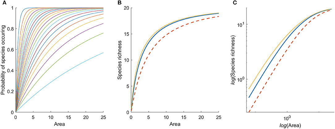
Figure 1. (A) Probability of occurrence of 20 species with random spatial distribution as a function of patch area. Different species have different densities in the habitat, which affects the slope of their respective curves. The mean densities for 20 species are simulated from a log-normal distribution with μ = −1.43, and σ = 1. (B) Species area relation generated by the model for a single habitat, under three different spatial aggregation patterns of individuals: spatial independence among individuals of the same species (solid blue), regular (dotted yellow), and aggregated spatial arrangement (dashed red). The solid blue curve is the sum of the probability curves in (A). (C) The species area relation on log-log scale.

Therefore, species richness, S_i, is also a concave function of area, i.e., it is increasing with area of the habitat patch and is bounded by 0 and K. Hence, a SAR is expected from basic probability theory (Figure 1B), and as there are only K species in the community, we also conclude that this SAR reaches an upper asymptote rather than increasing indefinitely (cf. Rosenzweig, 1995). It therefore cannot be approximated by a power-function and will not be linear on log-log scale (Figure 1C). This holds true irrespective of how individuals are spatially distributed within and among species.

To estimate species richness we need to make some explicit assumptions about the spatial distributions of individual organisms, and we will use three well-known and often applied distributions: Poisson, negative binomial, and binomial. If the number of individuals of a species found in a unit of area follows the Poisson distribution it is equivalent to assuming that each individual occurs independently of the whereabouts of other individuals within a habitat (Pielou, 1977). Although organisms will not be distributed independently of each other, this assumption is routinely made, e.g., when using Poisson regression techniques to analyze count data in ecological studies. For Poisson distributed organisms the probability to encounter at least one (i.e., not zero) individual of the species is

$\begin{array}{ll}{p}_{i,j}=1-e^{-a_i{m}_{i,j}},& (2)\end{array}$

since the expected number of individuals to encounter is a_im_i,j. The resulting SAR, as found by combining expressions 1 and 2, is shown by the solid curve in Figure 1B.

As two alternatives to spatial independence we may assume either a spatially aggregated or spatially regular distribution. If the individuals of a species are aggregated, their numbers per unit area may follow a negative binomial distribution, and hence

$\begin{array}{ll}{p}_{i,j}=1-{\left(\frac{k_j}{k_j+m_{i,j}}\right)}^{a_i{k}_j},& (3)\end{array}$

where k_j is the over-dispersion coefficient for the spatial distribution of the individuals of species j. Alternatively, if the organisms are more regularly dispersed (repulsed) the probability could be calculated from the binomial distribution:

$\begin{array}{ll}{p}_{i,j}=1-{\left(1-\frac{m_{i,j}}{n_j}\right)}^{a_i{n}_j},& (4)\end{array}$

where n_j is the maximum number of individuals of species j that can fit within a unit area. Note that in expressions 3 and 4, a_i cancels everywhere except in the exponents. The resulting SARs for all three distributions are shown in Figure 1B. We see that the underlying spatial distributions of the organisms affects the SAR, but not dramatically, and the general shape of the curve (decelerating toward an asymptote) is unaffected. If the individuals of species are evenly dispersed in space (binomial), more species are likely to be found in a small area, than if they are randomly dispersed (Poisson). If they are strongly aggregated (negative binomial), larger areas need to be included before all species are found.

For the Poisson distribution it is possible to simplify the algebra by using matrix notation and rewrite expression 1 as

$\begin{array}{ll}{S}_i=(1-e^{-a_i{\text{M}}_i})1.& (5)\end{array}$

Note that M_i is a single row matrix with the densities of all species in habitat i, m_i,j, as elements, and 1 is a K-length column vector of ones to accomplish the summation.

It follows from expressions 1 and 2 that the rate of change in species richness with area is

$\begin{array}{ll}\frac{\partial S}{\partial a_i}={\displaystyle \sum _{j=1}^K}{e}^{-a_i{m}_{i,j}}{m}_{i,j}=e^{-a_i{\text{M}}_i}{\text{M}}_{{}^i}^T,& (6)\end{array}$

(M${}_i^T$ is the transpose of M_i). This derivative tends to zero as area goes to infinity, i.e., the marginal species productivity of any habitat is decreasing in area.

Rather than estimating expected species richness, the model could be used to calculate other metrics of community composition or biodiversity, such as Shannon or Gini-Simpson diversities, or any other Hill-number (Hill, 1973; Jost, 2006), or β-diversities as species identity is maintained throughout the calculations and frequencies of all species can be calculated. However, for simplicity we limit the treatment to species richness in this paper.

Species Richness in Mosaic Landscapes

Species richness in a mosaic landscape is affected by the habitat mix and the extent of species overlap between different habitats. Thus, some species might occur in multiple habitats whilst others occur in single habitats.

With two habitats, expected species richness in the landscape, i.e., the number of species occurring in habitat 1 or habitat 2 or both, is therefore

$\begin{array}{ll}{S}_T={\displaystyle \sum _{j\in \left(I_1\cup I_2\right)}}\left(p_{1,j}+p_{2,j}-p_{1,j}{p}_{2,j}\right).& (7)\end{array}$

Here I₁ and I₂ are the subsets of species in habitat 1 and 2 respectively, and p_1,j p_2,j is the probability of species j occurring in both habitats, and hence this term eliminates the probability of species common to both habitats, which follows from basic set theory (Appendix S1). The calculation of expected species richness in the case of three or more habitats follows from 7 (the case of three habitats is shown in Appendix S1): it equals the sum of the probabilities of each species j occurring in each habitat i with area a_i in the landscape, adjusted for species overlap among habitats.

It may be convenient to substitute q_1,j for 1-p_1,j and q_2,j for 1-p_2,j in equation 7, such that

$\begin{array}{ll}{S}_T={\displaystyle \sum _{j\in \left(I_1\cup I_2\right)}}\left(\left(1-q_{1,j}\right)+\left(1-q_{2,j}\right)-\left(1-q_{1,j}\right)\left(1-q_{2,j}\right)\right)& (8)\end{array}$

which simplifies to

$\begin{array}{ll}{S}_T={\displaystyle \sum _{j\in \left(I_1\cup I_2\right)}}\left(1-q_{1,j}{q}_{2,j}\right)& (9)\end{array}$

That is, the probabilities to sum are simply the probabilities of each species not being absent from both habitats. In fact, this general result can be extended to any number of habitats (Appendix S1), but does require discrete habitat classes, and will not be easy to apply to habitat gradients without discretizing them.

For Poisson distributed organisms, q_1,j = $e^{-a_1{m}_{1,j}}$and q_2,j = $e^{-a_2{m}_{2,j}}$. Hence,

$\begin{array}{ll}{S}_T={\displaystyle \sum _{i\in \left(I_1\cup I_2\right)}}\left(1-e^{-\left(a_1{m}_{1,j}+a_2{m}_{2,j}\right)}\right),& (10)\end{array}$

which is equivalent to

$\begin{array}{ll}{S}_T=\left(1-e^{-\text{A}\text{M}}\right)1.& (11)\end{array}$

Here, the densities of all species in both habitats are in the matrix M, which has one row for each habitat and one column for each species, such that the total number of columns equals the combined species pool in both habitats (I₁ ∪ I₂). A species j which does not occur in habitat i will have m_i,j = 0. A is a single row matrix with habitat areas, a₁ and a₂. Note that expression 9 is general for any spatial distribution of organisms, whereas 10 and 11 are specific to densities following the Poisson distribution. Additionally, A can be extended with additional rows for each landscape for which calculations are being made.

We may also consider correlations in densities among species across habitats. If the correlation between habitats i and i′ (ρ_i,i′) is negative, then species that are common in one habitat are usually rare in the other.

In Figure 2A, we show an example of a landscape consisting of two habitats. The total species richness is given by the contours (isoquants), as a function of the areas of habitats 1 and 2. We assume that both habitats have a species pool of the same 100 species, but densities of species across habitats are uncorrelated, ρ_1,2 = 0, and average densities are the same in both habitats (Figure 2C). Increasing the area of any of the habitats will increase species richness, and naturally, an increase in habitat 1 will increase species richness by the same amount as an increase in habitat 2, i.e., ∂S_T/∂a₁= ∂S_T/∂a₂. These two partial derivatives are given by

$\begin{array}{ll}{S}^{\prime }=e^{-AM}{M}^T.& (12)\end{array}$

FIGURE 2

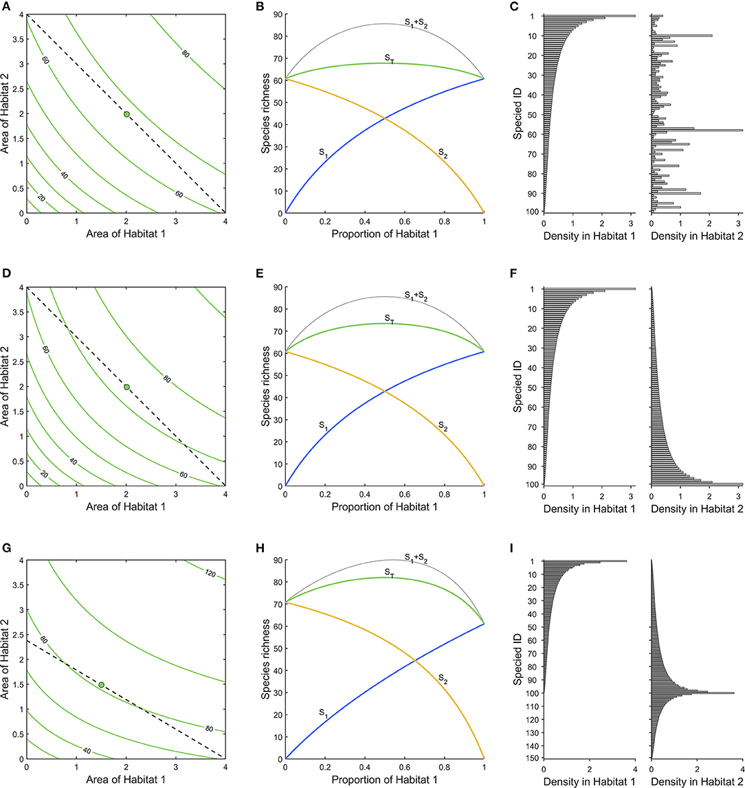
Figure 2. (A) Total species richness of the landscape (green), as a function of areas of the two habitats. A budget line (dashed) connects all points with four area units, and a green dot indicates maximum species richness along it. (B) S_T (green) is the net total species richness along the budget line in (A). S₁ (blue) and S₂ (yellow) are the gross number of species contributed by each habitat, and the curve S₁₊₂ (gray) is the sum of these curves (which overestimates S_T, ignoring overlap). (C) Densities of species in habitats. Species are ordered according to their density in habitat 1. Densities of species are simulated from log-normal distributions with μ = −1.43, σ = 1, and ρ = 0. (D–F) As (A–C), but with negatively correlated densities between habitats (ρ = −1), which makes the maximum total species richness, S_T, higher and the gradient toward it steeper. (G–I) As in (A–C), but negative correlation (ρ = −1) between densities and larger species pool in habitat 2 (note that species 101–150 are absent from habitat 1) strengthens the gradient in that habitat. Habitat 2 has the higher cost (shallow slope of budget line in G), canceling that effect and the optimum is still an equal mix of the two habitats.

That is, we obtain the steepest increase in species richness if we add the same areas of both habitats, as we assume uncorrelated and similar species densities, and the same species pools in both habitats (Figure 2C). Consequently, if a species can survive in different habitats, its probability of survival should be maximized through preserving a mix of these habitats, rather than maximizing the area of any single habitat. That is, generalists benefit from habitat diversity.

In Figures 2D–F the densities of species in the two habitats are perfectly negatively correlated (ρ_1,2 = −1; Figure 2F). However, the species pools for both habitats are identical. The results are similar to the previous case, but as the overlap between the habitats is less, species richness increases more by adding similar amounts of both habitats. This result is generated by the fact that there is the same number of specialists in both habitats.

Had the correlation between habitats been perfectly positive (ρ_1,2 = 1), the contours would have been straight lines; adding area of either habitat would have the same effect because in essence the two habitats are identical.

Constrained Optimization of Biodiversity

The dashed line in Figure 2A connects points with a constant total area, a₁ + a₂ = B = 4 (a “budget line”). In Figure 2B, we show the effect on species richness of varying habitat 1 as a proportion of the total area. Hence, Figure 2B renders the cross-section of Figure 2A along the dashed line starting at the upper left. This is the kind of situation we might have if we consider the distribution of different habitats within a fixed area of land (Cabeza and Moilanen, 2006). It arises when we have a piece of land of fixed size and want to consider what would be the consequence of converting one habitat in it to another (Pereira and Daily, 2006).

In Figure 2D, the corresponding situation is shown for the case with negatively correlated densities. With the current assumptions, of identical species pool and average densities in the two habitats, the highest species richness is achieved with equal proportions of the two habitats, just like in Figure 2B.

It is important to note that the difference between the curves S_T and S₁ + S₂ in Figures 2B,D is due to the species overlap. The curve for S₁ + S₂, i.e., the number of species found in 1 plus the number in 2, is the same in both figures. However, the total number of different species found in the two habitats taken together, S_T, is lower in Figure 2B, as there the overlap between the habitats is greater.

If land prices differ between the habitats the budget line will be affected. Assume habitat 1 costs c₁ per hectare and the price for habitat 2 is c₂. With a budget of B there is a constraint:

$\begin{array}{ll}B=a_1{c}_1+a_2{c}_2,& (13)\end{array}$

i.e., the total cost of preserving both habitats must be B, when weighting the habitat areas by their respective costs.

To solve the optimal allocation of habitats, in maximizing species richness under a budget constraint (regardless of whether prices are different or the same), we use the technique of Lagrange multipliers. The Lagrangian function is

$\begin{array}{ll}L=S_T-\lambda (a_1{c}_1+a_2{c}_2-B)& (14)\end{array}$

where λ is the Lagrange multiplier. The expression in parenthesis is hence the budget constraint, which needs to be zero when the budget is satisfied. To find an optimal combination of areas of the two habitats we additionally need both partial derivatives to satisfy ∂L/∂a₁= 0 and ∂L/∂a₂= 0. With the probability distributions of the organisms that we have used, it is not possible to analytically solve for a₁, a₂, and λ simultaneously. However, we know that at the optimum

$\begin{array}{ll}\lambda =\frac{1}{c_1}\frac{\partial S_T}{\partial a_1}=\frac{1}{c_2}\frac{\partial S_T}{\partial a_2},& (15)\end{array}$

which will occur where the budget line is tangent to a contour line. This tangency will also define the optimal solution. At that point, λ measures the shadow price of species (e.g., species per €), i.e., the marginal gain in species richness per unit increase in budget. The marginal value of habitat i is thus given by S′/c and the optimal decision to maximize species richness is to increase the area of (investment in) the habitat with the higher marginal value. This will hold true also for cases with more habitats than two.

In Figures 2G–I we show an effect of varying land prices of different habitats. The combined species pool of the two habitats is 150; all species occur in habitat 2, but only 100 of them in habitat 1, and the remaining 50 are entirely absent from habitat 1 (Figure 2I). In addition there is a perfect negative correlation between the densities of species in common in the two habitats, ρ_1,2 = −1, such that the most common species in habitat 1 is the rarest in habitat 2. This may represent a case where habitat 2 is a natural forest and habitat 1 is farmland, the converted habitat. Here, more species are gained by increasing the area of habitat 2, as it is the richer. However, as densities are negatively correlated some species will more likely occur in habitat 1. Here we have assumed that the more species-rich habitat 2 is also the more costly (c₁= 1, c₂= 1.68), and this offsets the difference in species richness, such that an equal mix between the habitats is again what maximizes biodiversity, given the limited budget (Figure 2H). If both habitats had the same price then a larger area of habitat 2 would be the optimal choice (cf. Figure 2G).

Data

During May-June of 2008, 2009, and 2011, we assessed bird densities using 5-min point counts in a total of 77 study landscapes in farmland in southernmost Sweden. Half of the landscapes were sampled in the “mixed farming region” and half in the “plains region.” Full details of the methods are provided by Stjernman et al. (2019) and in Appendix S2. Landscapes were either 2.5 × 2.5 km squares or 1 km radius circles (Appendix S2). In each landscape there were 16 survey points in a regular 4 by 4 grid covering the landscape. To ensure that field border habitat was sampled sufficiently, half of the points were displaced to the nearest field border. Points that fell in forest (>50 m from farmland) or in built up areas were not surveyed, as we are focusing on farmland, i.e., habitats that could be affected by agricultural policy (Stjernman et al., 2019). All birds seen or heard were identified and noted on high resolution aerial photos in the field and later digitized. Only birds observed ≤ 150 m from the observation point, were included in analyses, totaling 10,280 birds of 96 species.

We measured the farmland habitat in 150 m radius circles centered on each survey point, from GIS shapefiles containing the land use for each year (IACS; https://ec.europa.eu/agriculture/direct-support/iacs_en). As we only required a single mean habitat composition of landscapes for the current analyses, we averaged across all points and landscapes. We grouped land uses into six categories: annually tilled crops, ley, fallow, bioenergy crops, semi-natural pasture, and field border. The last category was estimated from field polygons' boundary lengths, assuming 1 m field border widths. Land uses other than farmland were ignored. Semi-natural pasture (hereafter called pasture) is a permanent, unimproved grassland, which can in principle be created from other habitats, but that is a slow and possibly costly process. Field borders in the studied regions often, but not always, have stonewalls and the vegetation is typically a mix of wild herbs, shrubs and some trees. In Sweden, removal of stonewalls is restricted by law, but increasing the area of field border is in principle a feasible conservation action. The other habitat types are more or less interchangeable, and may replace each other in crop rotations, except if the bioenergy crop is a woody plant, such as Salix.

The same six habitat classes were measured in 10 m radius circles centered on each observed bird. If a circle contained more than 10 m field border we assumed that the bird was sitting on the border, otherwise its observation was assigned to the habitats in the circle, in proportions relative to the areas covered by each habitat. By summing the habitat use of all birds within each species, and dividing by the total habitat areas inside all 150 m circles we obtained the densities of all species in each habitat.

We calculated an optimal mix of the six habitats at the landscape scale (Equations 14 and 15) by numerically finding the composition that minimized the standard deviation of the S′/c vector (cf. Equation 15), given the constraints that total area is always 200 ha and field edge could not account for more than 20 ha (see below). For this we used non-linear multivariate constrained minimization, using the function fmincon in MATLAB (www.mathworks.com), and MATLAB was also used for evaluating and illustrating the other parts of the model. In the Supplementary Data S1, we present R (R-Core-Team, 2018) code for the main part of the model, and an annotated R-script with a worked example is provided in the Supplementary Data S1.

Results

Figure 3 shows the densities of 96 bird species in six different habitats. Clearly, field borders have the overall highest densities, and densities across habitats are moderately correlated (Table 1). In Figure 4A we show an analysis, using expression 11, of a hypothetical example where a landscape can consist of up to 200 ha (2 km²) of either annually tilled fields or field borders, with the bird densities shown in Figure 3. The lower grayed triangle indicates where field borders are <10% of the total area, i.e., what might be observed in reality. The solid part of the budget line connects 200 ha landscapes with a maximum of 10% field border habitat, and the solid dot indicates the maximum species richness (~60) attainable with those constraints. Had it been possible to further increase the area of field borders to as much as e.g., 20%, expected bird species richness would increase to 67.5, but this is hardly a realistic landscape. However, the extreme with all 200 ha annually tilled and no borders is quite realistic but harbors only 21.3 species. Adding field borders to such a landscape (moving from right to left in Figure 4B) rapidly adds species. Figure 4C shows the marginal rate of change in species richness with a change in the area of annually tilled, i.e., how many species are lost for each additional hectare of annually tilled. Adding field borders to landscapes where there are none would increase species richness by 17.2 for the first hectare added (i.e., the negative of the marginal rate of change in species at 100% annually tilled in Figure 4C). If there are 4% field borders (and 96% annually tilled) in the landscape, corresponding to an average field size of 1 ha, the expected number of bird species is 51.0, and the marginal rate of loss of species richness with additional annually tilled would be 1.3 species per hectare (Figure 4C).

FIGURE 3

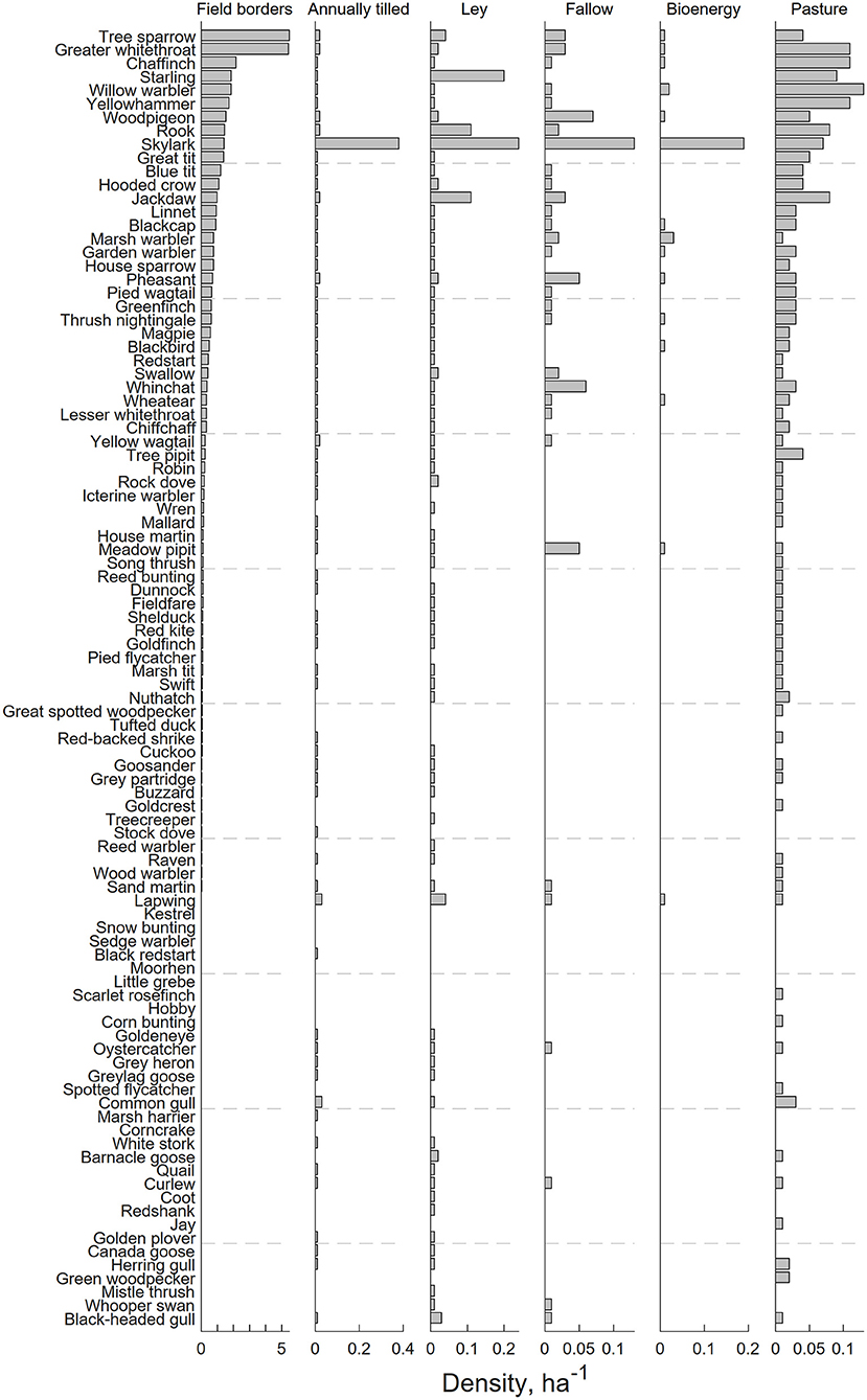
Figure 3. Densities of the 96 observed bird species in the six surveyed habitats. Species are ordered according to their density in field borders.

TABLE 1

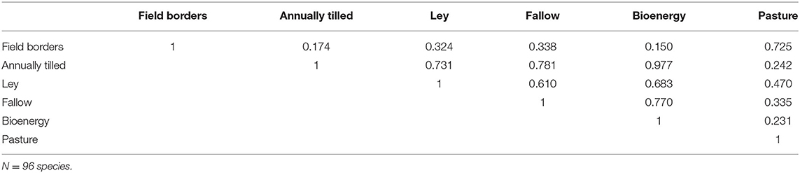
Table 1. Pearson correlations between densities of the observed birds in the different habitats.

FIGURE 4

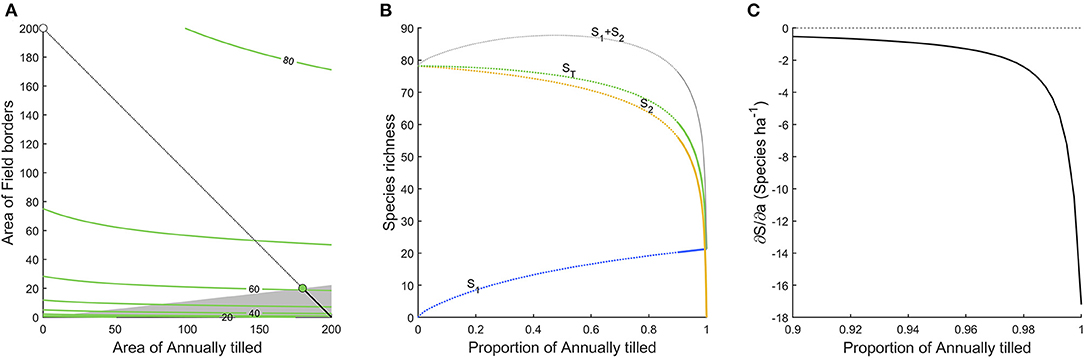
Figure 4. (A,B) as in Figure 2, but for the bird dataset, analyzing only annually tilled land and field borders. The radically higher densities of many species in field border means that the optimal landscape composition would be to have as much field border as possible. The gray shaded area in (A), and the solid parts of the curves in (B) indicate the cases where there is up to 10% of field border. (C) The marginal rate of change in species richness with a change in the area of annually tilled in the landscape.

The bird data were collected in two adjacent agricultural regions (Plains and Mixed, see Appendix S2) that differ in habitat composition (Figures 5A,B). Applying expression 11 again, expected bird species richness in landscapes of 200 ha with the average composition of each region, is 43.7 species in the plains, and 49.0 species in the mixed. Marginal species gain (expression 12) with increasing areas of pasture, and especially field borders, were positive in both regions, but higher in the plains (Figures 5A,B) as that region has less pasture and field borders, and lower species richness. Assuming equal conversion costs between all habitats, the best habitat composition (with field borders at the allowed maximum, 10%) is 60% pasture, and 30% ley (Figure 5C), based on the optimization analysis. With that habitat composition we would expect to find 65.7 species in a 200 ha landscape, and as the area of field borders was not allowed to vary freely, there was still a positive marginal gain of species with that habitat, as indicated by the yellow line in Figure 5C. If we assume twice the cost of creating semi-natural pastures in comparison to the other habitats, the new optimum would be to have only 36% pasture and increase ley to 54% (Figure 5D). This would reduce expected species richness very slightly to 65.3. Consequently, the optimal habitat configuration will be determined through the interplay among conversion costs and species productivity of the different habitats.

FIGURE 5

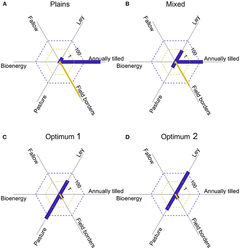
Figure 5. (A,B) show the area of the six habitats (blue bars), and the marginal rate of change in species richness with an increase in the respective area (yellow bars), for the two agricultural regions surveyed. Note that there are small positive yellow bars for pasture and ley in both (A,B). (C) Shows the results of an optimization, where the area of field border was constrained to ≤ 10%, and conversion costs were equal for all habitats. (D) is like (C), but with doubled cost to create pasture.

Discussion

Our main aim is to develop a tool for scenario analyses of expected species richness under resource constraints in mosaic landscapes. This allocation or trade-off problem is particularly relevant in human-modified landscapes, where conservation authorities (or policymakers) may have a wide range of alternative land uses or management practices to consider. For example, our model can evaluate which strategy along the land-sharing – land-sparing continuum that will maximize conservation of species under the constraint of maintaining agricultural production (c.f. Phalan et al., 2011). It may also inform about the optimal allocation of European Union agri-environment schemes to alternative measures under budget constraints (Wätzold et al., 2008). Not least, our model can be combined with land-use modeling, to evaluate biodiversity outcomes of policies with complex impacts, for example alternative formulations of the Common Agricultural Policy, where consequences of funding agri-environment schemes are related both to farmers' willingness to implement subsidized management and the structural change induced on agriculture by the policy (Brady et al., 2009). From a welfare-economic perspective, land uses should be allocated optimally, otherwise society will be wasting resources and biodiversity will be lower than possible (given resource constraints). Further, authorities need decision-support in the form of ex-ante evaluations or predictions of the potential impacts of policy designs on species richness, because program periods are usually long (5–7 years in the EU), and hence ex-post evaluations carried out long after policy implementation. Cost-effective conservation policy under these circumstances requires practical tools for predicting the potential impacts of different policy designs or interventions on biodiversity.

The model we have described is a general method for predicting the expected species richness in an area with a particular mix of different habitats. It results in a mechanistic model for a SAR based on first principles from probability theory, whereas previous models analyzing a similar kind of problem, i.e., species diversity in mosaic landscapes, have assumed a phenomenological functional form of a SAR (Pereira and Daily, 2006; Koh et al., 2010; Martins and Pereira, 2017; Keil et al., 2018). Data on species abundances in multiple habitat types can be “plugged in” into any of the expressions 11, 12, or 15 (Supplementary Data S1). These results can then be used to estimate expected species richness, habitat value, or the optimal habitat allocation, respectively, for maximizing species richness (Butsic and Kuemmerle, 2015). It should be noted, however, that when analyses are based on e.g., monitoring data that could include e.g., migrants, or when densities do not reflect carrying capacity (e.g., source-sink dynamics), results should be interpreted with extra caution.

In a homogeneous landscape, an approximation of the SAR can be used to predict the impact of habitat destruction on species richness (Koh et al., 2010). Species richness in a mosaic landscape, however, is also affected by the habitat mix and the extent of species overlap between habitats. Pereira and Daily (2006) define a countryside SAR as one that accounts for differential use of habitats by different species groups (rather than individual species). Our model is capable of predicting the impact of habitat alteration on species richness as well as keeping track of which individual species are most likely to disappear, whereas previous models require additional demographic modeling to discriminate between individual species (Martins and Pereira, 2017). Our model circumvents the need for a demographic model in the cases treated by us and by Martins and Pereira (2017), by being based upon the matrix of species densities in the different habitat types. This is not only more convenient, but also reduces the risk of compounding error. However, the simplicity of our model has a price: we assume mean densities to be fixed within habitat types, and currently the model does not incorporate e.g., direct area effects (such as thresholds), effects of isolation or spatial arrangement (cf. Fahrig, 2013, 2017; Haddad et al., 2017a), or population dynamics (see below). Adding fragmentation effects, such as making species' density m_ij dependent on area, is an important next step, and would likely make the SAR sigmoidal, and the S_T curve (Figure 2) more peaked.

Discrimination between individual species is important when all species are not valued equally in conservation objectives. For example, conserving important ecosystem services providers may be deemed important at local (α) scales even if they occur in many other sites, and the local preservation therefore does not contribute to large-scale (γ) species richness. Conversely, conserving nationally rare species may be deemed more important than our model would give at regional scales (Giljohann et al., 2018). With our model, it is possible to account for some species being of higher conservation concern than given from a simple tally of species, as it discriminates between species. Thus, it can be adapted to optimize species richness at alternative spatial scales by weighting the species probabilities according to their value at the most relevant scale, i.e., optimizing a weighted function between species value and γ-diversity. This is not possible using the classical or countryside SAR without additional steps. However, the focus of this paper is effects on landscape level species richness.

Benton et al. (2003) argue that habitat heterogeneity is “the key” to maintaining farmland biodiversity. Our results provide an explicit mechanism as to why heterogeneity might have a value in itself (Triantis et al., 2003). In general, a mix of habitats results in higher species richness if each habitat supports different species (Rafe et al., 1985). However, if a particular species can survive in different habitats, as is common in mosaic landscapes, the probability of species survival can be maximized by preserving some area of each habitat rather than a single habitat, because its marginal probability of survival is decreasing in area of each habitat (expression 13). Technically the sharing of habitat is therefore a sufficient condition to generate the curved species richness isoquants shown in Figure 2 and, hence an interior solution to the maximization problem given a total area constraint. An intuitive explanation is that since there is diminishing returns to species richness with increasing area of a single habitat (Figure 1), adding species from another habitat will in general maximize expected biodiversity. Similarly, our model returns high marginal values of habitats with complementary communities, even in small fragments (Figures 4, 5, cf. Wintle et al., 2019).

Our model is a significant step forward, but still has several limitations as it does not incorporate direct effects of scale, configuration, or interspecific interactions (Dunning et al., 1992; Andrén, 1994; Nicholson et al., 2006). In some cases it would be preferable to let density increase with area, and in a meta-population context one might assume thresholds, so that small or isolated patches are unlikely to have viable populations of some species (Andrén, 1994; Moilanen et al., 2005). However, this is context dependent, and often our assumptions are probably a reasonable approximation to reality. Furthermore, the probability of occurrence that our model relies on is an effect of population density and patch area, and should thus be positively related to persistence. Although it is beyond the scope of this paper, it would probably be feasible in the future, to modify this model to incorporate scale effects. For example, the model by Drechsler et al. (Drechsler and Johst, 2010; Drechsler et al., 2016) for population viability in habitat patches may be possible to combine with the current model. The current version of the model also only covers the process of habitat supplementation and not habitat complementation (Dunning et al., 1992; Fahrig et al., 2011), i.e., many animals' need of access to different habitats simultaneously (e.g., for nesting and foraging) in mosaic landscapes.

Our model is very simple to apply to a real dataset with densities of species in different habitats. We provided a simple illustrative example of this, demonstrating the differential value of conserving semi-natural pastures in two different landscape types if the objective is to maximize bird diversity at landscape scales. However, we provide this example mostly for illustrative purposes, and that deeper analyses are required to actually inform decisions of e.g., the formulation of agri-environment schemes, as we have not accounted for the constraints and time-delayed effects of converting one land-use type to another. For example pastures are normally permanent and difficult to recreate, but can sometimes be converted to arable or more likely subject to forest encroachment or plantations. By contrast, the removal of field borders, such as stonewalls, to enlarge arable land is prohibited by law in Sweden today, but was common practice until the 1970s. The way we include costs in the model assume that for a particular habitat, the cost is equal independent of its history of land use, whereas in reality there may be unequal costs of converting land use to and from a particular state. Such conversion costs could be added as fixed costs in the model (cf. Hart et al., 2014) and would result in path dependent outcomes. Also, some bird species are likely dependent on the interaction between habitats, such that some of the more extreme representation of landscapes (e.g., only field borders) that are theoretically possible, would render unrealistic results. Nevertheless, we show that with such a biodiversity dataset, it is straightforward to estimate the marginal value of each of the habitats. This value is expressed in terms of the number of species gained per unit increase in habitat area, or per monetary unit invested in it. This is crucial information when e.g., desiring to evaluate different management options and policy instruments that affect the areal extent of habitats and for allocating conservation budgets cost-effectively.

Data Availability Statement

The original contributions presented in the study are included in the article/Supplementary Material, further inquiries can be directed to the corresponding author.

Author Contributions

OO, MVB, and HGS conceived the idea. OO designed and developed the model with significant input from MVB on the economic theory, and improvement from MS. OO and HGS wrote the manuscript with significant input from MVB and MS. OO, MS, and HGS designed the field study. All authors contributed to the article and approved the submitted version.

Funding

This study was funded by grants from Formas to OO (2006-2076), HGS (210-2009-1680), and MS (226-2013-1204).

Conflict of Interest

The authors declare that the research was conducted in the absence of any commercial or financial relationships that could be construed as a potential conflict of interest.

Publisher's Note

All claims expressed in this article are solely those of the authors and do not necessarily represent those of their affiliated organizations, or those of the publisher, the editors and the reviewers. Any product that may be evaluated in this article, or claim that may be made by its manufacturer, is not guaranteed or endorsed by the publisher.

Acknowledgments

We thank Ulf Mörte, Ylva Hanell, Juliana Dänhardt, Petter Olsson, and Mikael Olofsson for help with collection of the bird field data.

Supplementary Material

The Supplementary Material for this article can be found online at: https://www.frontiersin.org/articles/10.3389/fcosc.2021.703260/full#supplementary-material

Appendix S1. Method for expanding the calculations for three and more habitats.

Appendix S2. Detailed description of field methods, including maps of study design.

Supplementary Data S1. Essential R code to perform the calculations of the central expressions 12 and 13, and analyze the bird dataset. Also replicates Figures 6, 7.

References

Andrén, H. (1994). Effects of habitat fragmentation on birds and mammals in landscapes with different proportions of suitable habitat - a review. Oikos 71, 355–366. doi: 10.2307/3545823

CrossRef Full Text | Google Scholar

Arrhenius, O. (1921). Species and area. J. Ecol. 9, 95–99. doi: 10.2307/2255763

CrossRef Full Text | Google Scholar

Benton, T. G., Vickery, J. A., and Wilson, J. D. (2003). Farmland biodiversity: is habitat heterogeneity the key? Trends. Ecol. Evol. 18, 182–188. doi: 10.1016/S0169-5347(03)00011-9

CrossRef Full Text | Google Scholar

Billionnet, A. (2011). Solving the probabilistic reserve selection problem. Ecol. Mod. 222, 546–554. doi: 10.1016/j.ecolmodel.2010.10.009

CrossRef Full Text | Google Scholar

Brady, M., Kellermann, K., Sahrbacher, C., Jelenik, L., and Lombianco, A. (2009). Impacts of decoupled support on farm structure, biodiversity and landscape mosaic: some EU results. J. Agric. Econ. 60, 563–585. doi: 10.1111/j.1477-9552.2009.00216.x

CrossRef Full Text | Google Scholar

Butsic, V., and Kuemmerle, T. (2015). Using optimization methods to align food production and biodiversity conservation beyond land sharing and land sparing. Ecol. Appl. 25, 589–595. doi: 10.1890/14-1927.1

PubMed Abstract | CrossRef Full Text | Google Scholar

Cabeza, M., and Moilanen, A. (2006). Replacement cost: a practical measure of site value for cost-effective reserve planning. Biol. Cons. 132, 336–342. doi: 10.1016/j.biocon.2006.04.025

CrossRef Full Text | Google Scholar

Chaudhary, A., and Brooks, T. M. (2019). National consumption and global trade impacts on biodiversity. World Dev. 121, 178–187. doi: 10.1016/j.worlddev.2017.10.012

PubMed Abstract | CrossRef Full Text | Google Scholar

Coleman, B. D. (1981). On random placement and species-area relations. Math. Biosci. 54, 191–215. doi: 10.1016/0025-5564(81)90086-9

CrossRef Full Text | Google Scholar

Dorazio, R. M., and Royle, J. A. (2005). Estimating size and composition of biological communities by modeling the occurrence of species. J. Am. Stat. Assoc. 100, 389–398. doi: 10.1198/016214505000000015

PubMed Abstract | CrossRef Full Text | Google Scholar

Dorazio, R. M., Royle, J. A., Söderström, B., and Glimskär, A. (2006). Estimating species richness and accumulation by modeling species occurrence and detectability. Ecology 87, 842–854. doi: 10.1890/0012-9658(2006)87842:ESRAAB2.0.CO

PubMed Abstract | CrossRef Full Text | Google Scholar

Drechsler, M., and Johst, K. (2010). Rapid viability analysis for metapopulations in dynamic habitat networks. Proc. Biol. Sci. R. Soc. 277, 1889–1897. doi: 10.1098/rspb.2010.0029

PubMed Abstract | CrossRef Full Text | Google Scholar

Drechsler, M., Smith, H. G., Sturm, A., and Wätzold, F. (2016). Cost-effectiveness of conservation payment schemes for species with different range sizes. Conserv. Biol. 30, 894–899. doi: 10.1111/cobi.12708

PubMed Abstract | CrossRef Full Text | Google Scholar

Dunning, J. B., Danielson, B. J., and Pulliam, H. R. (1992). Ecological processes that affect populations in complex landscapes. Oikos 65, 169–175. doi: 10.2307/3544901

CrossRef Full Text | Google Scholar

Egan, J. F., and Mortensen, D. A. (2012). A comparison of land-sharing and land-sparing strategies for plant richness conservation in agricultural landscapes. Ecol. Appl. 22, 459–471. doi: 10.1890/11-0206.1

PubMed Abstract | CrossRef Full Text | Google Scholar

Ekroos, J., Olsson, O., Rundlöf, M., Wätzold, F., and Smith, H. G. (2014). Optimizing agri-environment schemes for biodiversity, ecosystem services or both? Biol. Cons. 172, 65–71. doi: 10.1016/j.biocon.2014.02.013

CrossRef Full Text | Google Scholar

Eriksson, O., Cousins, S. A. O., and Bruun, H. H. (2002). Land-use history and fragmentation of traditionally managed grasslands in Scandinavia. J. Veg. Sci. 13, 743–748. doi: 10.1111/j.1654-1103.2002.tb02102.x

CrossRef Full Text | Google Scholar

Fahrig, L. (2013). Rethinking patch size and isolation effects: the habitat amount hypothesis. J Biogeography 40, 1649–1663. doi: 10.1111/jbi.12130

CrossRef Full Text | Google Scholar

Fahrig, L. (2017). Ecological responses to habitat fragmentation per se. Ann. Rev. Ecol. Evol. Syst. 48, 1–23. doi: 10.1146/annurev-ecolsys-110316-022612

CrossRef Full Text | Google Scholar

Fahrig, L., Baudry, J., Brotons, L., Burel, F. G., Crist, T. O., Fuller, R. J., et al. (2011). Functional landscape heterogeneity and animal biodiversity in agricultural landscapes. Ecol. Lett. 14, 101–112. doi: 10.1111/j.1461-0248.2010.01559.x

PubMed Abstract | CrossRef Full Text | Google Scholar

Frishkoff, L. O., Ke, A., Martins, I. S., Olimpi, E. M., and Karp, D. S. (2019). Countryside biogeography: the controls of species distributions in human-dominated landscapes. Curr. Landscape Ecol. Rep. 4, 15–30. doi: 10.1007/s40823-019-00037-5

CrossRef Full Text | Google Scholar

Giljohann, K. M., Kelly, L. T., Connell, J., Clarke, M. F., Clarke, R. H., Regan, T. J., et al. (2018). Assessing the sensitivity of biodiversity indices used to inform fire management. J. Appl. Ecol., 55, 461–471. doi: 10.1111/1365-2664.13006

CrossRef Full Text | Google Scholar

Haddad, N. M., Gonzalez, A., Brudvig, L. A., Burt, M. A., Levey, D. J., and Damschen, E. I. (2017a). Experimental evidence does not support the habitat amount hypothesis. Ecography. 40, 48–55. doi: 10.1111/ecog.02535

CrossRef Full Text | Google Scholar

Haddad, N. M., Holt, R. D. Jr, Fletcher, R. J., Loreau, M., and Clobert, J. (2017b). Connecting models, data, and concepts to understand fragmentation's ecosystem-wide effects. Ecography 40, 1–8. doi: 10.1111/ecog.02974

CrossRef Full Text | Google Scholar

Hannah, L., Carr, J. L., and Landerani, A. (1995). Human disturbance and natural habitat - a biome level analysis of a global data set. Biodiv. Cons., 4, 128–155. doi: 10.1007/BF00137781

CrossRef Full Text | Google Scholar

Hart, R., Brady, M., and Olsson, O. (2014). Joint production of food and wildlife: uniform measures or nature oases?. Environ. Resour. Econ. 59, 187–205.

Google Scholar

He, F., and Legendre, P. (1996). On species-area relations. Am. Nat. 148, 719–737. doi: 10.1086/285950

CrossRef Full Text | Google Scholar

Hill, M. O. (1973). Diversity and evenness: a unifying notation and its consequences. Ecology 54, 427–432. doi: 10.2307/1934352

CrossRef Full Text | Google Scholar

IPBES. (2019). Global Assessment Report on Biodiversity and Ecosystem Services of the Intergovernmental Science- Policy Platform on Biodiversity and Ecosystem Services. IPBES Secretariat, Bonn, Germany.

Google Scholar

Jost, L. (2006). Entropy and diversity. Oikos 113, 363–375. doi: 10.1111/j.2006.0030-1299.14714.x

CrossRef Full Text | Google Scholar

Ke, A., Sibiya, M. D., Reynolds, C., McCleery, R. A., Monadjem, A., and Fletcher, R. J. (2018). Landscape heterogeneity shapes taxonomic diversity of non-breeding birds across fragmented savanna landscapes. Biodiv. Cons. 27, 2681–2698. doi: 10.1007/s10531-018-1561-7

CrossRef Full Text | Google Scholar

Keil, P., Pereira, H. M., Cabral, J. S., Chase, J. M., May, F., Martins, I. S., et al. (2018). Spatial scaling of extinction rates: theory and data reveal nonlinearity and a major upscaling and downscaling challenge. Global Ecol. Biogeogr. 27, 2–13. doi: 10.1111/geb.12669

CrossRef Full Text | Google Scholar

Koh, L. P., Lee, T. M., Sodhi, N. S., and Ghazoul, J. (2010). An overhaul of the species-area approach for predicting biodiversity loss: incorporating matrix and edge effects. J Appl. Ecol. 47, 1063–1070. doi: 10.1111/j.1365-2664.2010.01860.x

CrossRef Full Text | Google Scholar

Leclère, D., Obersteiner, M., Barrett, M., Butchart, S. H. M., Chaudhary, A., De Palma, A., et al. (2020). Bending the curve of terrestrial biodiversity needs an integrated strategy. Nature 585, 551–556. doi: 10.1038/s41586-020-2705-y

PubMed Abstract | CrossRef Full Text | Google Scholar

Marques, A., Martins, I. S., Kastner, T., Plutzar, C., Theurl, M. C., Eisenmenger, N., et al. (2019). Increasing impacts of land use on biodiversity and carbon sequestration driven by population and economic growth. Nat. Ecol. Evol. 3, 628–637. doi: 10.1038/s41559-019-0824-3

PubMed Abstract | CrossRef Full Text | Google Scholar

Martins, I. S., and Pereira, H. M. (2017). Improving extinction projections across scales and habitats using the countryside species-area relationship. Sci. Rep. 7, 12899. doi: 10.1038/s41598-017-13059-y

PubMed Abstract | CrossRef Full Text

Matthews, T. J., Triantis, K. A., and Whittaker, R. J. (2021). The Species-Area Relationship: Theory and Application. Cambridge: Cambridge University Press.

Google Scholar

Mendenhall, C. D., Karp, D. S., Meyer, C. F. J., Hadly, E. A., and Daily, G. C. (2014). Predicting biodiversity change and averting collapse in agricultural landscapes. Nature 509:213. doi: 10.1038/nature13139

PubMed Abstract | CrossRef Full Text | Google Scholar

Moilanen, A., Franco, A. M., Early, R. I., Fox, R., Wintle, B., and Thomas, C. D. (2005). Prioritizing multiple-use landscapes for conservation: methods for large multi-species planning problems. Proc. Biol Sci. R. Soc. 272, 1885–1891. doi: 10.1098/rspb.2005.3164

PubMed Abstract | CrossRef Full Text | Google Scholar

Nicholson, E., Westphal, M. I., Frank, K., Rochester, W. A., Pressey, R. L., Lindenmayer, D. B., et al. (2006). A new method for conservation planning for the persistence of multiple species. Ecol. Lett. 9, 1049–1060. doi: 10.1111/j.1461-0248.2006.00956.x

PubMed Abstract | CrossRef Full Text | Google Scholar

Pereira, H. M., and Daily, G. C. (2006). Modeling biodiversity dynamics in countryside landscapes. Ecology 87, 1877–1885. doi: 10.1890/0012-9658(2006)871877:MBDICL2.0.CO

PubMed Abstract | CrossRef Full Text | Google Scholar

Pereira, H. M., Leadley, P. W., Proenca, V., Alkemade, R., Scharlemann, J. P. W., Fernandez-Manjarres, J. F., et al. (2010). Scenarios for global biodiversity in the 21st century. Science 330, 1496–1501. doi: 10.1126/science.1196624

PubMed Abstract | CrossRef Full Text | Google Scholar

Phalan, B., Onial, M., Balmford, A., and Green, R. E. (2011). Reconciling food production and biodiversity conservation: land sharing and land sparing compared. Science 333, 1289–1291. doi: 10.1126/science.1208742

PubMed Abstract | CrossRef Full Text | Google Scholar

Pielou, E. C. (1977). Mathematical Ecology. New York, NY: Wiley-Interscince.

Google Scholar

Polasky, S., Nelson, E., Lonsdorf, E., Fackler, P., and Starfield, A. (2005). Conserving species in a working landscape: land use with biological and economic objectives. Ecol. Appl. 15, 1387–1401. doi: 10.1890/03-5423

CrossRef Full Text | Google Scholar

Powers, R. P., and Jetz, W. (2019). Global habitat loss and extinction risk of terrestrial vertebrates under future land-use-change scenarios. Nat. Climate Change. 9:323. doi: 10.1038/s41558-019-0406-z

CrossRef Full Text | Google Scholar

Preston, F. W. (1962). The canonical distribution of commonness and rarity: part I. Ecology 43, 185–215. doi: 10.2307/1931976

CrossRef Full Text | Google Scholar

Rafe, R. W., Usher, M. B., and Jefferson, R. G. (1985). Birds on reserves: the influence of area and habitat on species richness. J Appl. Ecol. 22, 327–335. doi: 10.2307/2403167

CrossRef Full Text | Google Scholar

R-Core-Team. (2018). R: A Language and Environment for Statistical Computing. Vienna: R Foundation for Statistical Computing.

Google Scholar

Rosenzweig, M. L. (1995). Species Diversity in Time and Space. Cambridge: Cambridge University Press.

Google Scholar

Stjernman, M., Sahlin, U., Olsson, O., and Smith, H. G. (2019). Estimating effects of arable land use intensity on farmland birds using joint species modeling. Ecol. Appl. 29:e01875. doi: 10.1002/eap.1875

PubMed Abstract | CrossRef Full Text | Google Scholar

Tjørve, E. (2002). Habitat size and number in multi-habitat landscapes: a model approach based on species-area curves. Ecography 25, 17–24. doi: 10.1034/j.1600-0587.2002.250103.x

CrossRef Full Text | Google Scholar

Tjørve, E., Kunin, W. E., Polce, C., and Calf Tjørve, K. M. (2008). Species-area relationship: separating the effects of species abundance and spatial distribution. J. Ecol. 96, 1141–1151. doi: 10.1111/j.1365-2745.2008.01433.x

CrossRef Full Text | Google Scholar

Triantis, K. A., Mylonas, M., Lika, K., and Vardinoyannis, K. (2003). A model for the species-area-habitat relationship. J. Biogeogr. 30, 19–27. doi: 10.1046/j.1365-2699.2003.00805.x

CrossRef Full Text | Google Scholar

Wätzold, F., Lienhoop, N., Drechsler, M., and Settele, J. (2008). Estimating optimal conservation in the context of agri-environmental schemes. Ecol. Econ. 68, 295–305. doi: 10.1016/j.ecolecon.2008.03.007

CrossRef Full Text | Google Scholar

Wintle, B. A., Kujala, H., Whitehead, A., Cameron, A., Veloz, S., Kukkala, A., et al. (2019). Global synthesis of conservation studies reveals the importance of small habitat patches for biodiversity. Proc. Nat. Acad. Sci. 116, 909–914. doi: 10.1073/pnas.1813051115

PubMed Abstract | CrossRef Full Text | Google Scholar