Distance-Weighted Graph Neural Networks on FPGAs for Real-Time Particle Reconstruction in High Energy Physics

1. Introduction

At the CERN Large Hadron Collider (LHC), high-energy physics (HEP) experiments collect signals generated by the particles produced in high-energy proton collisions that occur every 25 ns, when two proton beams cross. The readout from the detectors that capture the particles emerging from the collision is filtered by a real-time processing system, known as the trigger, that discards uninteresting collision events, based on a set of predefined algorithms. The trigger system is structured in two stages: a Level-1 trigger (L1T), implemented with custom electronics on-detector and field-programmable gate arrays (FPGAs); and a high-level trigger (HLT), consisting of a computer farm, possibly including co-processor accelerators like graphics processing units (GPUs) and FPGAs. Because of asynchronous event processing at the HLT, the accept/reject decision has to be reached with a typical latency of $\mathcal{O}\left(100\right)\text{ms}$. However, at the L1T, a decision must be taken within a fixed latency of $\mathcal{O}\left(1\right)\mu \text{s}$. The main limitations are the synchronous, “hard-deadline” nature of the processing system and the limited size of the memory buffer for the data from each beam crossing.

While HLT algorithms have a complexity comparable to those used offline to produce the final physics results, a typical L1T algorithm consists of simpler rules based on coarser objects to satisfy the latency constraint. Consequently, the resolution of quantities computed at the L1T is typically poor compared to offline quantities. Recently, the successful deployment of the first machine learning (ML) L1T algorithm, based on a boosted decision tree (BDT), at the LHC (Acosta et al., 2018) has changed this tendency, raising interest in using ML inference as fast-to-execute approximations of complex algorithms with good accuracy. This first example consisted of a large, pre-computed table of input and output values implementing a BDT, which raises the question of how to deploy more complex architectures. This question motivated the creation of hls4ml (Duarte et al., 2018; Loncar et al., 2020), a library designed to facilitate the deployment of ML algorithms on FPGAs.

A typical hls4ml workflow begins with a neural network model that is implemented and trained using Keras (Keras, 2015), PyTorch (Paszke et al., 2019), or TensorFlow (Abadi et al., 2015). The trained model is passed to hls4ml, directly or through the ONNX (Bai et al., 2019) interface, and converted to C++ code that can be processed by a high-level synthesis (HLS) compiler to produce an FPGA firmware. By design, hls4ml targets low-latency applications. To this end, its design prioritizes all-on-chip implementations of the most common network components. Its functionality has been demonstrated with dense neural networks (DNNs) (Duarte et al., 2018), extended to also support BDTs (Summers et al., 2020). Extensions to convolutional and recurrent neural networks are in development. The library comes with handles to compress the model by quantization, up to binary and ternary precision (Di Guglielmo et al., 2020). Recently, support for QKeras (Qkeras, 2020) models has been added, in order to allow for quantization-aware training of models (Coelho et al., 2020). While the hls4ml applications go beyond HEP, its development has been driven by the LHC L1T use case.

Graph neural networks (GNNs) are among the complex architectures whose L1T implementations are in high demand, given the growing list of examples showing how well GNNs can deal with tasks related to HEP (Henrion et al., 2017; Choma et al., 2018; Abdughani et al., 2019; Arjona Martínez et al., 2019; Jin et al., 2019; Ju et al., 2019; Qasim et al., 2019b; Bernreuther et al., 2020; Moreno et al., 2020a; Moreno et al., 2020b; Qu and Gouskos, 2020; Shlomi et al., 2020). In fact, while the irregular geometry of a typical HEP detector complicates the use of computing vision techniques such as convolutional neural networks, GNNs can naturally deal with the sparse and irregular nature of HEP data.

In this work, we show how a graph model can be efficiently deployed on FPGAs to perform inference within $\mathcal{O}\left(1\right)\mu \text{s}$ for HEP-related problems. We consider the distance-weighted architecture GarNet, introduced in Qasim et al., (2019b), which is designed to keep resource consumption under control by reducing as much as possible the number of operations. It has been demonstrated to perform well for a HEP-related task, namely particle reconstruction in a calorimeter. For these reasons, it represents a good candidate for our purpose. The firmware implementation of GarNet presented in this work has been included in hls4ml, representing the first graph-based algorithm available in the library.

We present a case study of a neural network algorithm based on GarNet, applied to a task of identifying the nature of an incoming particle and simultaneously estimating its energy from the energy deposition patterns in a simulated imaging calorimeter. The inference accuracy of the firmware implementation of the algorithm is compared against its offline counterpart running on processors (CPUs and GPUs). Latency and resource utilization of the translated FPGA firmware are reported, along with a discussion on their implications for real-world usage of similar algorithms.

This paper is structured as follows. In Section 2, we briefly recount related work. Section 3 defines the main problem by outlining the challenges in designing a graph network compatible with L1T latency and resource constraints. Section 4 describes how GarNet addresses these challenges, and introduces a simplified form of the algorithm with a better affinity to a firmware implementation. The case study using a calorimeter simulation is presented in Section 5, with detailed descriptions of the task setup, model architecture, training results, and the summary of FPGA firmware synthesis. Finally, conclusions are given in Section 6.

2. Related Work

Graph neural networks are gaining interest in HEP applications, mainly due to their intrinsic advantage in dealing with sparse input datasets, which are very common in HEP. A recent review of applications of GNNs to HEP problems may be found in Shlomi et al., (2020). In particular, dynamic GNNs (Qasim et al., 2019b; Wang et al., 2019; Gray et al., 2020; Kieseler, 2020) are relevant for particle reconstruction tasks, such as tracking (Ju et al., 2019) and calorimetry (Qasim et al., 2019b).

Development of ML models deployable to FPGA-based L1T systems is helped by tools for automatic network-to-circuit conversion such as hls4ml. Using hls4ml, several solutions for HEP-specific tasks (e.g., jet tagging) have been provided (Duarte et al., 2018; Coelho et al., 2020; Di Guglielmo et al., 2020; Summers et al., 2020), exploiting models with simpler architectures than what is shown here. This tool has been applied extensively for tasks in the HL-LHC upgrade of the CMS L1T system, including an autoencoder for anomaly detection, and DNNs for muon energy regression and identification, tau lepton identification, and vector boson fusion event classification (CMS Collaboration, 2020). However, prior to this work, GNN models had not yet been supported by hls4ml. To the best of our knowledge, the present work is the first demonstration of GNN inference on FPGAs for a HEP application.

Outside of HEP, hardware and firmware acceleration of GNN inference, and graph processing in general, has been an active area of study in recent years, motivated by the intrinsic inefficiencies of CPUs and GPUs when dealing with graph data (Besta et al., 2019; Gui et al., 2019). Nurvitadhi et al., 2014; Ozdal et al., 2016; Auten et al., 2020; Geng et al., 2020; Kiningham et al., 2020; Yan et al., 2020; Zeng and Prasanna, 2020 describe examples of GNN acceleration architectures. Auten et al., 2020; Geng et al., 2020; Yan et al., 2020; Zeng and Prasanna, 2020. are specific to the graph convolutional network (GCN) (Kipf and Welling, 2017), while the graph inference processor (GRIP) architecture in Kiningham et al., (2020) is efficient across a wide range of GNN models. All five architectures are designed for processing graphs with millions of vertices under a latency constraint (10–1,000$\mu \text{s}$ or more) that is less stringent than in the HEP L1T environment (less than 1$\mu \text{s}$), and are thus not directly applicable to our use case. Nurvitadhi et al., (2014) and Ozdal et al., (2016) present frameworks that automatically generate register-transfer level (RTL) implementations for graph computations according to user-defined configurations. While these frameworks are applicable to various graph processing tasks, they require the user to specify the design in highly specific nonstandard format, rather than a standard serialized ML model as in our implementation.

3. General Requirements and Challenges

In the framework of Battaglia et al., (2018), a graph is a triplet $\left(\upsilon ,\mathrm{ℰ},\mathcal{u}\right)$, where $\mathrm{\upsilon }$ is a set of entities (vertices) each possessing some attributes in a fixed format, $\mathrm{ℰ}$ is a set of pairwise relations (edges) between the elements in $\mathrm{\upsilon }$, potentially possessing some additional attributes, and $\mathcal{u}$ are global (graph-level) attributes. While a GNN can be any neural network that acts on such graphs, in this work we specifically consider graph networks (GN) (Battaglia et al., 2018), i.e., architectures that consist of repeatable graph-to-graph mapping blocks (GN blocks). Each GN block performs some combination of operations such as edge feature transformation, aggregation of neighbors’ features at each vertex, vertex feature transformation, global aggregation of edge and vertex features, and global feature transformation. A GN takes a graph as an input sample, where the cardinality of $\upsilon$ may differ sample to sample, and infers its properties, which may be anything from a global scalar, such as a classification label of the sample, to new edge attributes.

To be usable as a part of an LHC L1T system, an algorithm must execute within $\mathcal{O}\left(1\right)\mu \text{s}$ and have the throughput to accept all inputs from each beam crossing every 25$\text{ns}$. Time-multiplexing, whereby N copies of the algorithm accept inputs from N different beam crossings, may be used to decrease the throughput requirement by a factor of N. Additionally, there is a practical constraint that the firmware implementation should fit in the FPGA resources of the system, i.e., utilize the resources such as digital signal processing units (DSPs), look-up tables (LUTs), flip-flips (FFs), and block RAM (BRAM) within the limits of chips available on the market. Satisfying these requirements with a GNN can be challenging for multiple reasons listed below.

• Model depth: Within each GN block, vertices exchange information with other directly connected vertices or with global attributes. Therefore, to expand the receptive field of each vertex beyond the nearest neighbors, multiple GN blocks must be repeated in the network. Given that various transformations within each GN block are often themselves multilayer perceptrons (MLPs), GNN models tend to be quite deep. Deep networks go against the latency requirement, as each perceptron layer uses at least one clock cycle on an FPGA under a straightforward implementation, and also against the resource usage requirement, because MLPs utilize multiplications heavily.

• Input size: Typically, for problems where the application of GNNs is interesting, the cardinality of $\mathrm{\upsilon }$ is at least $\mathcal{O}\left({10}^2\right)$. Even with the high degree of parallelism of FPGAs, due to finiteness of the compute resource, such large input will have to be processed serially to a certain extent, increasing the latency and the interval before a new input can be accepted, known as the initiation interval (II). Longer IIs lead to lower throughput values.

• Memory usage: Related to the problem of the input size, if the algorithm requires temporary retention of features for all vertices or edges, memory usage may be prohibitive for an FPGA firmware implementation.

• Memory access pattern: Except for certain cases, algorithms that have both $\upsilon$ and $\mathrm{ℰ}$ in the input usually require random memory access, for example when reading or writing features of vertices at the ends of the edges. This poses a challenge in FPGA firmware design not only because it implies that there needs to be a large enough memory bank to store all vertex and/or edge data, but also because random memory access itself is a costly operation (Besta et al., 2019). The exceptions include when $\mathrm{ℰ}$ is trivial ($\mathrm{ℰ}=\varnothing$ or when the graph is complete) and when all samples have an identical graph topology. In such cases, the memory access pattern of the algorithm is known at compile time and therefore can be statically scheduled in the FPGA firmware.

The case of $\mathrm{ℰ}=\varnothing$ is a rather extreme solution to the last challenge, but it is also attractive in terms of memory usage. In fact, even without explicit input edge features, a GNN can infer regional and non-local properties of the graph by globally gathering the vertex features and then scattering the gathered information back to the vertices. This information flow can also be mediated by a learnable attention mechanism (Veličković et al., 2018). The attention mechanism suppresses information from vertices that are considered unimportant, effectively forming “soft” edges among the unsuppressed vertices.

In the next section, we study a GNN architecture with these exact properties, then discuss the modifications to the architecture to make it suitable for an FPGA firmware implementation.

4. A Simplified GARNET Layer in the HLS4ML Framework

In this work, we consider GarNet (Qasim et al., 2019b) as a specific example of GNN. A GarNet layer is a GN block that takes as input a set of V vertices, each possessing $F_{\text{in}}$ features, and returns the same set of vertices with $F_{\text{out}}$ features. In a GarNet layer, $F_{\text{in}}$ features of each vertex are encoded into an internal representation and gathered at S aggregators. A distance parameter between each of the aggregators and vertices is also computed from the vertex attributes. Information gathered at the aggregators are then sent back to individual vertices and decoded into $F_{\text{out}}$ features. Communications between the vertices and aggregators are weighted by a decreasing function of the distance parameter, implementing an attention mechanism that allows the network to learn a dynamic, nontrivial graph structure from the vertex input alone.

The original GarNet algorithm, while already using less compute and memory resource than other similar GNN architectures in Qasim et al., (2019b) and Wang et al., (2019), is still challenging to implement as fast and high-throughput FPGA firmware. The biggest problem arises from the use of the input feature vector as a part of the input to the decoder, which requires retention of the input data until the last steps of the algorithm. An immediate consequence of this requirement is a longer II, because processing of new samples cannot start while the input data for the current sample is still in use. Furthermore, the input feature vector is already used to compute the distance parameter as well as the internal representation of each vertex, and therefore a reuse of the input in the decoder creates a complex data flow, restricting the options for pipelining the algorithm.

We therefore designed a modified GarNet algorithm with a simplified processing flow:

• Input transformation (Figures 1A,B): An encoder network converts the features $g_v^j\left(j=1,\dots ,F_{\text{in}}\right)$ of the $v^{\text{th}}$ vertex $\left(v=1,\dots ,V\right)$ into an internal learned representation vector $f_v^i\left(i=1,\dots ,F_{\text{LR}}\right)$. In parallel, another network (distance calculator) also acts on $g_v^j$ and computes the distance parameters $d_{av}\left(a=1,\dots ,S\right)$ between the vertices and the S aggregators. Implicitly, this means that a complete bipartite graph with $VS$ edges is built from $\mathrm{\upsilon }$ and , where is the set of aggregators (Figure 1B). The encoder and distance calculator networks are both single-layer perceptrons with linear activation functions, so one can write them as linear transformations

$f_v^i={\displaystyle \sum _{j=1}^{F_{\text{in}}}{w}_j^i\hspace{0.17em}{g}_v^j}+b^i(1)$

$d_{av}={\displaystyle \sum }_{j=1}^{F_{\text{in}}}{\alpha }_{aj}\hspace{0.17em}{g}_v^j+{\beta }_a ,(2)$

where $\left(w_j^i,b^i\right)$ and $\left({\alpha }_{aj},{\beta }_a\right)$ are the kernels and biases of the encoder and distance calculator networks, respectively.

• Aggregation (Figure 1C): The learned representation vectors $f_v^i$ of the vertices are weighted by a potential function $W_{av}=\text{exp}\left(-d_{av}^2\right)$ and averaged across the vertices. In other words, the ith averaged feature $h_a^i$ of aggregator a is written as

$h_a^i=\frac{1}{V_{\text{max}}}{\displaystyle \sum }_{v=1}^V{W}_{av}{f}_v^i.(3)$

The factor $V_{\text{max}}$ in the denominator is the maximum possible value for the vertex multiplicity V (as V may have a different value for each input sample). Through this normalization by a common factor, the information about the size of the sample (cardinality of $\upsilon$) is effectively encoded into $h_a^i$.

• Output transformation (Figures 1D,E): The aggregated features are sent back to the vertices using the same weights as

${\tilde{f}}_{av}^i=W_{av}\hspace{0.17em}{h}_a^i,(4)$

and then transformed by a single-layer decoder network with linear activation function into the final output representation $g_v^{\prime k}\left(k=1,\dots ,F_{\text{out}}\right)$. With the kernel u and bias c of the decoder, this is written as

$g_v^{\prime k}={\displaystyle \sum }_{i=1}^{F_{\text{LR}}}{\displaystyle \sum }_{a=1}^S{u}_{ia}^k\hspace{0.17em}{\tilde{f}}_{av}^i+c^k.(5)$

This simplified algorithm differs from the original design in the following ways. First, only the mean over vertices is computed at the aggregators, whereas the maximum is also used in the original design. In other words, the aggregators in the original design have

$h_a^{\prime i}=\underset{v}{\text{max}}{W}_{av}{f}_v^i(6)$

as an additional set of features. Secondly, as already noted, the input feature vector is not used as a part of the input to the decoder network. In the original GarNet design, the decoder is expressed as

$g_v^{\prime k}={\displaystyle \sum }_{i=1}^{F_{\text{LR}}}{\displaystyle \sum }_{a=1}^S{W}_{av}\left(u_{ia}^k\hspace{0.17em}{h}_a^i+u_i^{\prime k}{h}_a^{\prime i}\right)+{\displaystyle \sum }_{i=1}^{F_{\text{in}}}{w}_i^{\prime k}{g}_v^i+c^k,(7)$

with additional sets of kernel weights $u^{\prime }$ and $w^{\prime }$. Finally, the original design applies a nonlinear ($\text{tanh}$) activation function to the decoder, while the simplified version uses a linear activation. In the specific case considered in the next section, these simplifications result in negligible degradation of the network performance. In the remainder of this paper, this simplified version of the algorithm is referred to as GarNet.

FIGURE 1

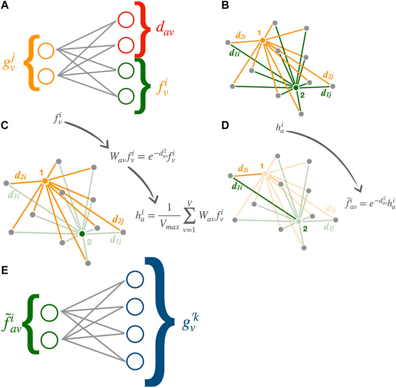
FIGURE 1. Processing flow of the modified GarNet algorithm: (A) The input features $\left(g_v^j\right)$ of each vertex are processed by a linear network, that returns a new set of features $\left(f_v^i\right)$ and its distance from the S aggregators $\left(d_{av}\right)$. (B) A graph is built in the learned space, using the $d_{av}$ distances. (C) A message is gathered by each aggregator, as a weighted sum across the vertices of $f_v^i$, with $W_{av}=\text{exp}\left(-d_{av}^2\right)$ as weights. (D) A message from each aggregator (${\tilde{f}}_{av}^i$) is passed back to each vertex, with the same $W_{av}$ weight. (E) The aggregated outputs of each vertex are given as input to a neural network, which returns the learned representation.

It is worth pointing out that while the GarNet layer uses only linear activation functions for all of the internal neural networks, it can still learn nonlinear functions through the nonlinearity of the potential function $W_{av}$. On the other hand, having no nonlinear activation functions allows a compact FPGA firmware implementation of the layer, consisting mostly of multiplications and additions. The only substantial computation comes with the exponential function, whose values can be pre-computed with sufficient granularity and stored.

An FPGA firmware implementation of the GarNet layer using Vivado (O’Loughlin et al., 2014) HLS is integrated into the hls4ml library. The HLS source code is written in C++ and is provided as a template, from which an HLS function for a GarNet layer can be instantiated, specifying the configurable parameters such as S, $F_{\text{LR}}$, and $F_{\text{out}}$. In the following, we provide some noteworthy details of the implementation.

In the HLS source code of GarNet, all quantities appearing in the computation are expressed as either integers or fixed-point numbers with fractional precision of at least eight bits. In particular, the distance parameter $d_{av}$ is represented with three integer bits, eight fractional bits, and one sign bit. During the layer computation, $d_{av}$ is reinterpreted as a 12-bit unsigned integer, which is used to retrieve the corresponding pre-computed value of $W_{av}$ from a table with 4,096 entries.

The processing flow in Eqs 1–5 is compactified in the hls4ml implementation by exploiting the linearity of the encoder, average aggregation, and the decoder. Equations 1, 3, and 5 can be combined into

$g_v^{\prime k}={\displaystyle \sum }_{a=1}^S{W}_{av}\left({\displaystyle \sum }_{j=1}^{F_{\text{in}}}{\tilde{w}}_{ja}^k{G}_a^j+{\tilde{b}}_a^k{L}_a\right)+c^k,(8)$

where

${\tilde{w}}_{ja}^k={\displaystyle \sum }_{i=1}^{F_{\text{LR}}}{u}_{ia}^k{w}_j^i,{\tilde{b}}_a^k={\displaystyle \sum }_{i=1}^{F_{\text{LR}}}{u}_{ia}^k{b}^i,G_a^j=\frac{1}{V_{\text{max}}}{\displaystyle \sum }_{v=1}^V{W}_{av}\hspace{0.17em}{g}_v^j,\text{and}\hspace{0.17em}{L}_a=\frac{1}{V_{\text{max}}}{\displaystyle \sum }_{v=1}^V{W}_{av}.(9)$

In particular, the kernel and bias tensors of the encoder and decoder are contracted into $\tilde{w}$ and $\tilde{b}$ at logic synthesis time, resulting in fewer steps to arrive at the output from the input.

With this simplification, the input data from each sample are encoded into $W_{av}$, $G_a^j$, and $L_a$. Therefore, a new sample can be processed as soon as the three quantities from the previous sample are computed. In other words, the II of the overall GarNet layer depends on the number of clock cycles needed to compute the three quantities. Furthermore, $G_a^j$ and $L_a$ can be derived trivially from $W_{av}$, making the latency of the computation of the latter the critical determinant of the throughput of the algorithm.

The computation of $W_{av}$ is performed independently on each vertex, and is therefore parallelizable across the vertices. In a fully parallelized implementation, there would be $V_{\text{max}}$ logic units (one unit per vertex) operated simultaneously. However, with V typically as large as $\mathcal{O}\left({10}^2\right)$ or greater, this configuration would consume too much of the FPGA resources and would not fit on a single chip. Therefore, the hls4ml implementation of GarNet allows a partial parallelization of the algorithm controlled by a parameter called the reuse factor ($R_{\text{reuse}}$). For $R_{\text{reuse}}>1$, the logic unit to compute $W_{av}$ is cloned $V_{\text{max}}/R_{\text{reuse}}$ times, such that each unit is reused serially up to $R_{\text{reuse}}$ times. This serial reuse is fully pipelined with the local II of one clock cycle. The latency $T_W$ for computing $W_{av}$ for all vertices is therefore given by

$T_W=T_W^0+R_{\text{reuse}},(10)$

where $T_W^0\sim 20$ is the number of clock cycles needed to compute $W_{av}$ for one vertex. The value of $T_W^0$ depends on the numerical precision of the fixed-point numbers in the computation.

Finally, the kernel and bias of the encoder and the kernel of the decoder can be quantized, such that each element takes only values $-1$, 0, or 1 (ternary quantization) (Zhu et al., 2017). In the quantized version of the algorithm, contracted kernel and bias $\tilde{w}$ and $\tilde{b}$ have elements that are $\mathcal{O}\left(1\right)$ integers. Multiplication of small integers with fixed-point numbers can be performed in FPGAs using LUTs rather than DSPs, which are usually the more scarce resource. Multiplications with LUTs also proceed faster than those with DSPs.

5. Case Study: Particle Identification and Energy Regression in an Imaging Calorimeter

As a case study, the hls4ml implementation of GarNet is applied to a representative task for the LHC L1T, namely reconstructing electrons and pions in a simulated 3D imaging calorimeter. In the following, we first describe the dataset used for the study, then define the task and the architectures of the ML models, and present the inference performance of the models and the resource usage of the synthesized firmware.

5.1. Dataset

The calorimeter is a multi-layered full-absorption detector with a geometry similar to the one described in Qasim et al., (2019b). The detector is made entirely of tungsten, which is considered as both an absorber and a sensitive material, and no noise or threshold effects in the readout electronics are simulated. While this homogeneous calorimeter design is not a faithful representation of a modern sampling calorimeter, this simplification allows us to evaluate the performance of the ML models decoupled from detector effects.

The calorimeter extends 36 cm in x and y and has a total depth in z of 2 m, corresponding to approximately 20 nuclear interaction lengths and 170 radiation lengths. The coordinate origin is placed at the center of the front face of the calorimeter. The calorimeter is segmented into 50 layers along z, with each layer divided into small square cells in the x-y plane, forming a three-dimensional imaging detector. Cells are oriented so their sides are parallel to the x and y axes. Tiling of the cells in each layer is uniform except for in one quadrant, where the cell sides are half as long as those in the other area. The aim of the tiling is to incorporate the irregularity of the geometry of a real-life particle physics calorimeter. The quadrant with smaller cells and the remainder of the layer are respectively called the high granularity (HG) and low granularity (LG) regions. The first 25 layers in z correspond to the electromagnetic calorimeter, with a layer thickness of 1 cm and cell dimensions of 2.25 cm $\times$ 2.25 cm in the HG region (4.5 cm $\times$ 4.5 cm in LG). The remaining 25 layers correspond to the hadron calorimeter, with a layer thickness of 7 cm and cell dimensions of 3 cm $\times$ 3 cm in the HG region (6 cm $\times$ 6 cm in LG). Schematics of the cell tiling in the electromagnetic and hadron parts are shown in Figure 2. The geometry and the detector response to particles are simulated using Geant4 (Agostinelli et al., 2003).

FIGURE 2

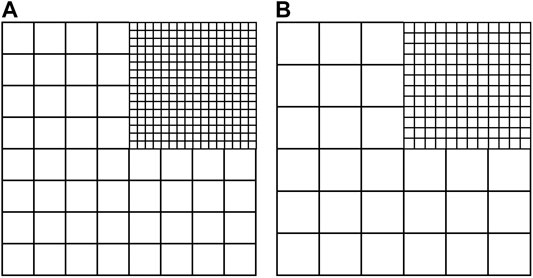
FIGURE 2. Schematics of the high-granularity and low-granularity regions of the (A) electromagnetic and (B) hadron layers.

Each event used in this study contains a high-energy primary particle and low-energy pileup particles, which represent backgrounds from simultaneous additional proton-proton interactions. The primary particle is either an electron (${\text{e}}^{-}$) or a charged pion (${\pi }^{\pm }$), shot at the calorimeter with momentum aligned along the z axis, i.e., perpendicular to the front face of the calorimeter. The x and y coordinates of the particle’s origin are randomly sampled according to a uniform distribution in a 10 cm $\times$ 10 cm region centered at $x=y=0$. Following this procedure, we aim to mimic a realistic situation in which the actual calorimeter extends to a much larger surface and the area covered by the geometry used in this study represents a portion of it. The value of the particle momentum is drawn randomly for each event from a uniform distribution between 10 and 100 GeV. The pileup particles consist of photons (γ) and ${\pi }^{\pm }$. The number of pileup particles is randomly sampled from a Poisson distribution with a mean of 40, with the ${\pi }^{\pm }$ multiplicity fixed to twice the γ multiplicity. This setup approximates the flux of pileup particles expected at a pseudorapdity $\eta =2$ in a $\text{Δ}\eta \times \text{Δ}\varphi =0.4\times 0.4$ patch of the forward region of an LHC detector during the High-Luminosity LHC (HL-LHC) phase (Apollinari et al., 2017). The momentum direction and the window of origin of the pileup particles are the same as the primary particle. The momentum value of the pileup particles is sampled from a Landau distribution with $\mu =0.6$ GeV and $c=0.5$ GeV, in a range of 0–20 GeV.

The output of the simulation for each event is the array of total energy deposition values by the particles at individual detector cells (hits). Energy depositions by the particles in the homogeneous calorimeter are recorded exactly, i.e., the detector output does not require calibration and is not affected by stochastic noise.

In an L1T system, hits containing energy depositions from a potentially interesting particle would be identified through a low-latency clustering algorithm. The clustering algorithm used in this study mimics the one planned for the L1T system of the HGCAL detector in CMS (CMS Collaboration, 2017a). In this approach, the hit with the largest energy deposition in the event is elected to be the seed, and the cluster consists of all hits contained in a cylinder whose axis passes through the center of the seed cell and extends along the z direction. The radius of the cylinder is set at 6.4 cm so that the resulting cluster contains 95% of the energy of the primary particle for 50% of the pion events. Because electromagnetic showers have a narrower energy spread than hadronic showers in general, all of the electron events have at least 95% of the energy contained in the same cylinder. Typical events with momenta of the primary particles around 50 GeV and the total pileup energy close to the median of the distribution are shown in Figures 3A and 3B. The hits in the figure are colored by the fraction of the hit energy due to the primary particle (primary fraction, $f_{\text{prim}}$) to help the visualization.

FIGURE 3

FIGURE 3. Examples of electron (A), (C) and pion (B), (D) events. Values in parentheses in the graph titles are the respective energy depositions contained in the cluster around the seed hit. Points represent hits in the detector, with their coordinates at the center of the corresponding detector cells and the size of the markers proportional to the square root of the hit energy. Opaque points are within the cluster, while the translucent ones are not. In (A) and (B), the point color scale from blue to red corresponds to the primary fraction (see Section 5.1 for definition). In (C) and (D), the color scale from blue to green corresponds to $\text{Δ}{E}_{\text{pred}}/\text{Δ}h$, which is an indication of the importance the neural network model places to individual hits for energy regression. See Section 5.3 for details.

The actual dataset used in this study thus contains one cluster per sample, given as an array of hits in the cluster, and one integer indicating the number of hits in the sample. Only the hits with energy greater than 120 MeV are considered. Each cluster contains at most 128 hits, sorted by hit energy in decreasing order. Note that sorting of the hit has no effect on the neural network, and is only relevant when truncating the list of hits to consider smaller clusters, as explored later. In fact, 0.2% of the events resulted in clusters with more than 128 hits, for which the lowest energy hits were discarded from the dataset. Each hit is represented by four numbers, corresponding to the hit coordinates, given in x, y, and z, and energy. The x and y coordinates are relative to the seed cell. The dataset consists of 500,000 samples, split evenly and randomly into ${\text{e}}^{-}$ and ${\pi }^{\pm }$ events, stored as NumPy (van der Walt et al., 2011; Harris et al., 2020) arrays in HDF5 format (The HDF Group, 2020). The dataset together with the ground truth information is available on the Zenodo platform (Iiyama and Kieseler, 2020).

5.2. Task and Model Architecture

The task in this study is to identify the nature of the primary particle and to simultaneously predict its energy, given the hits in the cluster. The ability to reliably identify the particle type and estimate its energy at the cluster level in a local calorimeter trigger system greatly enhances the efficacy of high-level algorithms, such as particle-flow reconstruction (ALEPH Collaboration, 1995; ATLAS Collaboration, 2017; CMS Collaboration, 2017b), downstream in the L1T system. However, because of the distortion of the energy deposition pattern in the cluster due to pileup, particle identification based on collective properties of the hits, such as the depth of the energy center of mass, can achieve only modest accuracy. Furthermore, only half of the pion events have 95% of the energy deposition from the pion contained in the cluster, requiring substantial extrapolation in the energy prediction. This task is thus both practically relevant and sufficiently nontrivial as a test bench of a GarNet-based ML model.

The architecture of the model is as follows. First, the input data represented by a two-dimensional array of $V_{\text{max}}\times F_{\text{in}}$ numbers per cluster are processed by a stack of three GarNet layers. The parameters $\left(S,F_{\text{LR}},F_{\text{out}}\right)$ for the first two layers are $\left(\mathrm{4,8,8}\right)$ and for the last layer are $\left(\mathrm{8,16,16}\right)$. The output of the third GarNet layer is averaged across the vertices for each of the 16 features. The resulting array of 16 numbers is then passed through two fully connected layers with 16 and 8 nodes and ReLU (Agarap, 2018) activation. Data flow is split into two branches in the final step. The first branch consists of a fully connected layer with a single node, whose output is activated by a sigmoid function and is interpreted as the classification prediction, i.e., the predicted probability that the primary particle is an electron. The other branch also consists of a single-node fully connected layer, but with a linear activation of the output, which is interpreted as the predicted value of the energy of the particle.

This model is built in Keras (Keras, 2015), using the corresponding implementation of GarNet available in Qasim et al., (2019a). In total, the model has 3,402 trainable parameters (2,976 in the three GarNet layers), whose values are optimized through a supervised training process using the Adam optimizer (Kingma and Ba, 2014). Input is processed in batches of 64 samples during training. The overall objective function that is minimized in the training is a weighted sum of objective functions for the classification and regression tasks:

$\mathrm{ℒ}=\beta {\mathrm{ℒ}}_{\text{class}}+\left(1-\beta \right){\mathrm{ℒ}}_{\text{reg}}(11)$

with $\beta =0.01$. The objective function for classification ${\mathrm{ℒ}}_{\text{class}}$ is the binary cross entropy in each batch between the truth labels (electrons are represented by 1 and pions by 0) and the classification output of the model. The objective function for regression ${\mathrm{ℒ}}_{\text{reg}}$ is the batch mean of the relative squared error

${\mathrm{ℒ}}_{\text{reg}}={[\left(E_{\text{pred}}-E_{\text{true}}\right)/E_{\text{true}}]}^2,(12)$

where $E_{\text{pred}}$ and $E_{\text{true}}$ are the predicted and true energies of the primary particle, respectively. The training is performed on 400,000 training and 100,000 validation samples over a few hundred epochs, with early stopping when the value of the objective function does not improve for ten consecutive epochs. Keeping the full training dataset on RAM and using two NVIDIA GeForce RTX 2080 Ti GPUs in parallel, each epoch takes roughly 30 s to process.

Additionally, we prepare a model in which the encoders and decoders of the GarNet layers are quantized as ternary networks using QKeras (Coelho et al., 2020; Qkeras, 2020), which performs quantization-aware training with the straight-through estimator by quantizing the layers during a forward pass but not a backward pass (Courbariaux et al., 2015; Zhou et al., 2016; Moons et al., 2017; Coelho et al., 2020). In the following, this model is referred to as the quantized model, and the original model as the continuous model. The quantized model is trained with the same objective function and training hyperparameters as the continuous model.

To evaluate the inference performance of the trained models, reference algorithms are defined separately for the classification and regression subtasks. The reference algorithm for classification (cut-based classification) computes the energy-weighted mean $\overline{z}$ and standard deviation ${\sigma }_z$ of the z coordinates of the hits,

$\overline{z}=\frac{{{{\displaystyle \sum }}^{\text{}}}_{i=1}^V{z}_i{h}_i}{{{{\displaystyle \sum }}^{\text{}}}_{i=1}^V{h}_i}\text{and}{\sigma }_z=\sqrt{\frac{{{{\displaystyle \sum }}^{\text{}}}_{i=1}^V{\left(z_i-\overline{z}\right)}^2{h}_i}{{{{\displaystyle \sum }}^{\text{}}}_{i=1}^V{h}_i}},(13)$

where i is the index of hits in the cluster and $z_i$ and $h_i$ are the z coordinate and energy of the ith hit. The cluster is labeled as an electron if $\overline{z}<{\overline{z}}^{\text{cut}}$ and ${\sigma }_z<{\sigma }_z^{\text{cut}}$, where ${\overline{z}}^{\text{cut}}$ and ${\sigma }_z^{\text{cut}}$ are predefined thresholds. Pions, and hadrons in general, tend to penetrate deeper in an absorbing detector and create showers of secondary particles with a larger transverse size than electrons and photons. For regression, the reference algorithm (weight-based regression) predicts the energy of the primary particle through a formula

$E_{\text{pred}}^{\text{ref}}={\displaystyle \sum }_{i=1}^V{w}_{l\left(i\right)}\left(h_i+b_{l\left(i\right)}\right),(14)$

where $l\left(i\right)$ is the detector z layer of hit i. Parameters $\left\{w_l,b_l\right\}\left(l=1,\dots ,50\right)$ are determined by minimizing ${\mathrm{ℒ}}_{\text{reg}}$ over the training dataset using $E_{\text{pred}}^{\text{ref}}$ as the predicted energy. Particle identification based on the energy deposition profile of the cluster and energy estimation based on weighted sum of hit energies are both common strategies in the conventional, non-ML-based event reconstruction approaches.

5.3. Training Result

Performance of the trained continuous and quantized models, evaluated using the validation sample, are shown in Figure 4. For each ML model, the inference results based on the original Keras model and the HLS model, converted using hls4ml, are shown. The HLS model provides a realistic emulation of the synthesized FPGA firmware.

FIGURE 4

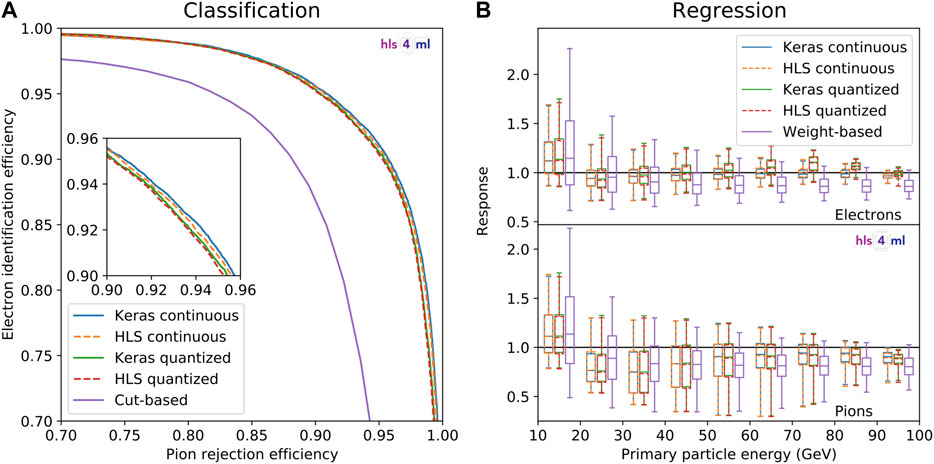
FIGURE 4. Classification (A) and regression (B) inference performance of the continuous and quantized GarNet-based models and the reference algorithms. Results from the Keras and HLS implementations are shown for the GarNet-based models. The classification performance is quantified with a ROC curve of electron identification efficiency vs. pion rejection efficiency. The inset in (A) shows a close-up view of the efficiency range 0.90–0.96 for both axes. The regression performance is quantified as the response $\left(E_{\text{pred}}/E_{\text{true}}\right)$ in 10 GeV bins of $E_{\text{true}}$. The horizontal line in the box corresponds to the median of the distribution, the top and bottom of the box to the upper and lower quartiles, and the upper and lower ends of the whiskers to the 95th and 5th percentiles.

The classification performance is given in terms of receiver operating characteristic (ROC) curves that trace the electron identification efficiency (true positive fraction) and pion rejection efficiency (true negative fraction) for different thresholds of the classifiers. The two GarNet-based models perform similarly and better than the cut-based reference in terms of the electron identification efficiency for a given pion rejection efficiency. A detailed comparison of the four sets of results from the GarNet-based models in the inset reveals that the continuous model performs slightly better than the quantized model, and that the difference between the Keras and HLS implementations is smaller for the quantized model.

The regression performance is given in terms of the response $\left(E_{\text{pred}}/E_{\text{true}}\right)$. Distributions of the response are summarized in 10 GeV bins of $E_{\text{true}}$, separately for the continuous model, quantized model, and the weight-based reference. In each summary, the horizontal line in the box corresponds to the median of the distribution, the top and bottom of the box to the upper and lower quartiles, and the upper and lower ends of the whiskers to the 95th and 5th percentiles. The GarNet-based models exhibit narrower spreads of the response distributions in most of the bins, with the continuous model again performing slightly better than the quantized model.

The differences between the Keras and HLS implementations are due to the numerical precision in the computation. While the former represents all fractional numbers in 32-bit floating-point numbers, the latter employs fixed-point numbers with bit widths of at most 18. Consequently, for the quantized model, where the encoder and decoder of the GarNet layers employ integer weights for inference, the difference between the two implementations are smaller.

For both subtasks, the GarNet-based models generally outperform the reference algorithms. The reference algorithm has narrower spread of the response in some energy bins for the regression subtask. However, it is important to note that the weights and biases appearing in Eq. 14 are optimized for a specific pileup profile, while in a real particle collider environment, pileup flux changes dynamically even on the timescale of a few hours. In contrast, algorithms based on inference of properties of individual hits, such as the GarNet-based models presented in this study, are expected to be able to identify hits due to pileup even under different pileup environments and thus to have a stable inference performance with respect to change in pileup flux. Since a detailed evaluation of application-specific performance of GarNet is not within the scope of this work, we leave this and other possible improvements to the model architecture and training to future studies.

To verify that GarNet can infer relations between individual vertices without edges $\mathrm{ℰ}$ in the input, the following test is performed. Using the two events shown in Figure 3, the energy of each hit in the clusters is increased one at a time by 10%, and the inference with the continuous model is performed for each perturbed event. If the model has learned to perfectly distinguish the primary particle from pileup at the vertex level, a small change in the energy of a hit from pileup should result in no change in the predicted particle energy. In Figures 3C and 3D, each hit in the cluster is colored by the ratio of the change of predicted particle energy and the amount of perturbation ($\text{Δ}{E}_{\text{pred}}/\text{Δ}h$). While some hits with $f_{\text{prim}}=0$ appear with $\text{Δ}{E}_{\text{pred}}/\text{Δ}h>0$, a general correspondence between $f_{\text{prim}}$ and $\text{Δ}{E}_{\text{pred}}/\text{Δ}h$ is observed. The occurrence of $\text{Δ}{E}_{\text{pred}}/\text{Δ}h>1$ is expected, given the extrapolation required to predict the full particle energy from the energy of the hits included in the cluster. With this test, we are able to probe how the GarNet-based model is learning the structure of the graph.

5.4. Model Synthesis and Performance

The latency, II, and resource usage of the FPGA firmware synthesized from the HLS implementations are summarized in Table 1. Vitis Core Development Kit 2019.2 (Kathail, 2020) is used for synthesis, with a Xilinx Kintex UltraScale FPGA (part number xcku115-flvb2104-2-i) as the target device and a clock frequency of 200 MHz. The reported resource usage numbers reflect the synthesis estimates from Vivado HLS. The latency and II reported here are the maximum values for samples with full $V_{\text{max}}$ vertices; the actual HLS implementation allows early termination of the serial reuse of the vertex-processing logic unit for samples with fewer vertices. The area under the ROC curve (AUC) and overall response root mean square (RMS) are used to summarize the performance.

TABLE 1

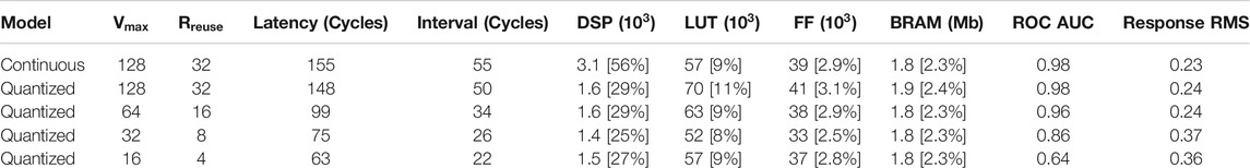
TABLE 1. Summary of the latency, II, FPGA resource usage metrics, and inference accuracy metrics of the synthesized firmware. The reported resource usage numbers reflect the synthesis estimates from Vivado HLS. The target FPGA is a Xilinx Kintex UltraScale FPGA (part number xcku115-flvb2104-2-i), which has 5,520 DSPs, 663,360 LUTs, 1,326,720 FFs, and 77.8 Mb of BRAM (Xilinx, 2020). The utilized percentage of the targeted FPGA resources are denoted in the square brackets.

Comparing the continuous and quantized models with $V_{\text{max}}=128$, the former has a longer latency and II and consumes substantially more DSPs. On the other hand, the quantized model uses more LUTs, mainly for the multiplications in the GarNet encoders and decoders, as discussed in Section 4. However, it is known that the expected LUT usage tend to be overestimated in Vivado HLS, while the expected DSP usage tends to be accurate (Duarte et al., 2018; Di Guglielmo et al., 2020). The DSP usage of $3.1\times {10}^3$ for the continuous model is well within the limit of the target device, but is more than what is available on a single die slice ($2.8\times {10}^3$) (Xilinx, 2020). The quantized model fits in one slice in all metrics. Given the small difference in the inference performance between the two models, it is clear that the quantized model is advantageous for this specific case study.

The latency of the synthesized quantized model at 148 clock periods, corresponding to 740$\text{ns}$, satisfies the LHC L1T requirement of $\mathcal{O}\left(1\right)\mu \text{s}$ execution. However, the II of 50 clock periods (250$\text{ns}$) implies that the logic must be time-multiplexed tenfold to be able to process a single cluster per LHC beam crossing period of 25$\text{ns}$. With $\mathcal{O}\left(100\right)$ or more clusters expected per beam crossing in the collision environment of HL-LHC, the throughput of the synthesized firmware is therefore inadequate for a reasonably sized L1T calorimeter system with $\mathcal{O}\left(100\right)$ FPGAs, and requires down-scoping or implementation improvements.

The simplest down-scoping measure is to reduce the size of the input. This is effective because the most prominent factor driving both the latency and the II of the firmware is $R_{\text{reuse}}$ (see Eq. 10), which in turn is determined by $V_{\text{max}}$ to be able to fit the logic in a single chip. To test how short the II can be made while retaining a reasonable inference performance, additional models with $V_{\text{max}}=64$, 32, and 16 are trained and synthesized into FPGA firmware. Clusters with more hits than $V_{\text{max}}$ are truncated by discarding the lowest energy hits. The fraction of truncated clusters for the three $V_{\text{max}}$ values are 27%, 85%, and 99%, respectively.

The results of synthesis of the additional models are given in the last three rows of Table 1. The values of FPGA resource usage metrics are similar in all quantized models because the ratio $V_{\text{max}}/R_{\text{reuse}}$ is kept at 4. The area under the ROC curve (AUC) and the root-mean-square (RMS) of the response are considered as metrics for the inference performance. Only a modest degradation of performance is observed by truncating the clusters to $V_{\text{max}}=64$, while the II is reduced by 16 clocks as a direct result of the reduction of $R_{\text{reuse}}$ by the same amount. This working point might thus represent a reasonable compromise between the inference performance and throughput. Further cluster truncation results in considerable loss of inference accuracy. It is also clear that reduction of $R_{\text{reuse}}$ has a diminishing return in terms of shorter II, and improvements to other parts of the algorithm are necessary to further reduce the II.

6. Conclusion

In this paper, we presented an implementation of a graph neural network algorithm as FPGA firmware with $\mathcal{O}\left(1\right)\mu \text{s}$ execution time. General considerations and challenges in implementing graph neural networks for real-time trigger systems at particle collider experiments are outlined, along with how algorithms such as GarNet address these issues. We then described the simplified version of GarNet, which is now available as a general-purpose graph network layer in the hls4ml library. An example use case of a machine learning model based on the simplified version of GarNet, applied to data from a simulation of a small imaging calorimeter, is presented. The model is able to learn to predict the identity and the energy of the particles detected at the calorimeter with high accuracy, while its firmware implementation executes in 740$\text{ns}$ and fits easily in a commercially available FPGA. Although the throughput of the firmware is not sufficient to make the model readily deployable in a submicrosecond, real-time collider trigger system, its variants with reduced input size are shown to have higher throughput with reasonable inference performance. These results demonstrate that fast inference of graph neural networks in FPGAs is possible, and with hls4ml, various graph-based machine learning architectures can be automatically translated into firmware.

Data Availability Statement

The datasets presented in this study can be found in online repositories. The names of the repository/repositories and accession number(s) can be found below: https://doi.org/10.5281/zenodo.3992780, doi:10.5281/zenodo.3992780. Simulation data set and the KERAS source code used for the case study are available on the Zenodo platform (Iiyama, 2020).

Author Contributions

All authors listed have made a substantial, direct, and intellectual contribution to the work and approved it for publication.

Funding

MP, AG, KW, SS, VL and JN are supported by the European Research Council (ERC) under the European Union’s Horizon 2020 research and innovation program (Grant Agreement No. 772369). SJ, ML, KP, and NT are supported by Fermi Research Alliance, LLC under Contract No. DE-AC02-07CH11359 with the U.S. Department of Energy (DOE), Office of Science, Office of High Energy Physics. PH is supported by a Massachusetts Institute of Technology University grant. ZW is supported by the National Science Foundation under Grants Nos. 1606321 and 115164. JD is supported by DOE Office of Science, Office of High Energy Physics Early Career Research program under Award No. DE-SC0021187. CERN has provided the open access publication fee for this paper.

Conflict of Interest

The authors declare that the research was conducted in the absence of any commercial or financial relationships that could be construed as a potential conflict of interest.

Acknowledgments

We acknowledge the Fast Machine Learning collective as an open community of multi-domain experts and collaborators. This community was important for the development of this project.

References

Abadi, M., Agarwal, A., Barham, P., Brevdo, E., Chen, Z., Citro, C., et al. (2015). TensorFlow: large-scale machine learning on heterogeneous distributed systems. Available at: http://download.tensorflow.org/paper/whitepaper2015.pdf.

CrossRef Full Text | Google Scholar

Abdughani, M., Ren, J., Wu, L., and Yang, J. M. (2019). Probing stop pair production at the LHC with graph neural networks. J. High Energy Phys. 8, 55. doi:10.1007/JHEP08(2019)055

CrossRef Full Text | Google Scholar

Acosta, D., Brinkerhoff, A., Busch, E., Carnes, A., Furic, I., Gleyzer, S., et al. (2018). “Boosted decision trees in the Level-1 muon endcap trigger at CMS,” in Proceedings, 18th international workshop on advanced computing and analysis techniques in physics research (ACAT 2017), Seattle, WA, August 21–25, 2017 (Seattle, WA: ACAT), 042042. doi:10.1088/1742-6596/1085/4/042042

CrossRef Full Text | Google Scholar

Agarap, A. F. (2018). Deep learning using rectified linear units (ReLU). [Preprint]. Available at: https://arxiv.org/abs/1803.08375.

CrossRef Full Text | Google Scholar

Agostinelli, S., Allison, J., Amako, K., Apostolakis, J., Araujo, H., Arce, P., et al. (2003). Geant4—a simulation toolkit. Nucl. Instrum. Methods Phys. Res. 506, 250. doi:10.1016/S0168-9002(03)01368-8

CrossRef Full Text | Google Scholar

ALEPH Collaboration (1995). Performance of the ALEPH detector at LEP. Nucl. Instrum. Methods Phys. Res. 360, 481. doi:10.1016/0168-9002(95)00138-7

CrossRef Full Text | Google Scholar

Apollinari, G., Béjar Alonso, I., Brüning, O., Fessia, P., Lamont, M., Rossi, L., et al. (2017). High-luminosity large hadron collider (HL-LHC): technical design report V. 0.1, CERN Yellow Reports: Monographs (Geneva, Switzerland: CERN). doi:10.23731/CYRM-2017-004

CrossRef Full Text | Google Scholar

Arjona Martínez, J., Cerri, O., Pierini, M., Spiropulu, M., and Vlimant, J. R. (2019). Pileup mitigation at the Large Hadron Collider with graph neural networks. Eur. Phys. J. Plus 134, 333. doi:10.1140/epjp/i2019-12710-3

CrossRef Full Text | Google Scholar

ATLAS Collaboration (2017). Jet reconstruction and performance using particle flow with the ATLAS detector. Eur. Phys. J. C 77, 466. doi:10.1140/epjc/s10052-017-5031-2

CrossRef Full Text | Google Scholar

Auten, A., Tomei, M., and Kumar, R. (2020). “Hardware acceleration of graph neural networks,” in 57th ACM/IEEE Design Automation Conference (DAC), San Francisco, CA, July 20–24, 2020 (San Francisco, CA: IEEE), 1–6. doi:10.1109/DAC18072.2020.9218751

CrossRef Full Text | Google Scholar

Bai, J., Lu, F., and Zhang, K. (2019). ONNX: open neural network exchange. Available at: https://github.com/onnx/onnx (Accessed August 20, 2020).

CrossRef Full Text | Google Scholar

Battaglia, P. W., Hamrick, J. B., Bapst, V., Sanchez-Gonzalez, A., Zambaldi, V., Malinowski, M., et al. (2018). Relational inductive biases, deep learning, and graph networks. [Preprint]. Available at: https://arxiv.org/abs/1806.01261.

CrossRef Full Text | Google Scholar

Bernreuther, E., Finke, T., Kahlhoefer, F., Krämer, M., and Mück, A. (2020). Casting a graph net to catch dark showers. [Preprint]. Available at: https://arxiv.org/abs/2006.08639.

CrossRef Full Text | Google Scholar

Besta, M., Stanojevic, D., De Fine Licht, J., Ben-Nun, T., and Hoefler, T. (2019). Graph processing on FPGAs: taxonomy, survey, challenges. [Preprint]. Available at: https://arxiv.org/abs/1903.06697.

CrossRef Full Text | Google Scholar

Choma, N., Monti, F., Gerhardt, L., Palczewski, T., Ronaghi, Z., Prabhat, , et al. (2018). Graph neural networks for IceCube signal classification. [Preprint]. Available at: https://arxiv.org/abs/2006.10159.

CrossRef Full Text | Google Scholar

CMS Collaboration (2017a). The phase-2 upgrade of the CMS endcap calorimeter. CMS Technical Design Report CERN-LHCC-2017-023. CMS-TDR-019 (Geneva, Switzerland: CERN).

CrossRef Full Text | Google Scholar

CMS Collaboration (2017b). Particle-flow reconstruction and global event description with the CMS detector. J. Instrum. 12, P10003. doi:10.1088/1748-0221/12/10/P10003

CrossRef Full Text | Google Scholar

CMS Collaboration (2020). The phase-2 upgrade of the CMS level-1 trigger. CMS Technical Design Report CERN-LHCC-2020-004. CMS-TDR-021 (Geneva, Switzerland: CERN).

CrossRef Full Text | Google Scholar

Coelho, C. N., Kuusela, A., Zhuang, H., Aarrestad, T., Loncar, V., Ngadiuba, J., et al. (2020). Automatic deep heterogeneous quantization of Deep Neural Networks for ultra low-area, low-latency inference on the edge at particle colliders. [Preprint]. Available at: https://arxiv.org/abs/2006.10159.

CrossRef Full Text | Google Scholar

Courbariaux, M., Bengio, Y., and David, J. P. (2015). “BinaryConnect: training deep neural networks with binary weights during propagations,” in Advances in neural information processing systems 28. Editors C. Cortes, N. D. Lawrence, D. D. Lee, M. Sugiyama, and R. Garnett (Red Hook, NY: Curran Associates, Inc.), 3123.

CrossRef Full Text | Google Scholar

Di Guglielmo, G., Duarte, J., Harris, P., Hoang, D., Jindariani, S., Kreinar, E., et al. (2020). Compressing deep neural networks on FPGAs to binary and ternary precision with hls4ml. Mach. Learn. Sci. Technol. 2, 015001. doi:10.1088/2632-2153/aba042

CrossRef Full Text | Google Scholar

Duarte, J., Han, S., Harris, P., Jindariani, S., Kreinar, E., Kreis, B., et al. (2018). Fast inference of deep neural networks in FPGAs for particle physics. J. Instrum. 13, 07027. doi:10.1088/1748-0221/13/07/P07027

CrossRef Full Text | Google Scholar

Geng, T., Li, A., Shi, R., Wu, C., Wang, T., Li, Y., et al. (2020). AWB-GCN: a graph convolutional network accelerator with runtime workload rebalancing. [Preprint]. Available at: https://arxiv.org/abs/1908.10834.

CrossRef Full Text | Google Scholar

Gray, L., Klijnsma, T., and Ghosh, S. (2020). A dynamic reduction network for point clouds. [Preprint]. Available at: https://arxiv.org/abs/2003.08013.

CrossRef Full Text | Google Scholar

Gui, C. Y., Zheng, L., He, B., Liu, C., Chen, X. Y., Liao, X. F., et al. (2019). A survey on graph processing accelerators: challenges and opportunities. J. Comput. Sci. Technol. 34, 339. doi:10.1007/s11390-019-1914-z

CrossRef Full Text | Google Scholar

Harris, C. R., Millman, K. J., van der Walt, S. J., Gommers, R., Virtanen, P., Cournapeau, D., et al. (2020). Array programming with NumPy. Nature 585, 357. doi:10.1038/s41586-020-2649-2

PubMed Abstract | CrossRef Full Text | Google Scholar

Henrion, I., Cranmer, K., Bruna, J., Cho, K., Brehmer, J., Louppe, G., et al. (2017). “Neural message passing for jet physics,” in Deep learning for physical sciences workshop at the 31st conference on neural information processing systems, Long Beach, CA, April 2017 (Long Beach, CA: NIPS), 1–6.

CrossRef Full Text | Google Scholar

Iiyama, Y. (2020). Keras model and weights for GARNET-on-FPGA. Available at: https://zenodo.org/record/3992780.

CrossRef Full Text | Google Scholar

Iiyama, Y., and Kieseler, J. (2020). Simulation of an imaging calorimeter to demonstrate GARNET on FPGA. Available at: https://zenodo.org/record/3888910.

CrossRef Full Text | Google Scholar

Jin, C., Chen, Sz., and He, H. H. (2019). Classifying the cosmic-ray proton and light groups on the LHAASO-KM2A experiment with the graph neural network. [Preprint]. Available at: https://arxiv.org/abs/1910.07160.

CrossRef Full Text | Google Scholar

Ju, X., Farrell, S., Calafiura, P., Murnane, D., Prabhat, , Gray, L., et al. (2019). Graph neural networks for particle reconstruction in high energy physics detectors. Available at: https://ml4physicalsciences.github.io/files/NeurIPS_ML4PS_2019_83.pdf.

CrossRef Full Text | Google Scholar

Kathail, V. (2020). “Xilinx vitis unified software platform,” in 2020 ACM/SIGDA international symposium on field-programmable gate arrays, New York, NY, March 2020 (New York, NY: Association for Computing Machinery), 173. doi:10.1145/3373087.3375887

CrossRef Full Text | Google Scholar

Keras Special Interest Group (2015). Keras. Available at: https://keras.io (Accessed August 20, 2020).

CrossRef Full Text | Google Scholar

Kieseler, J. (2020). Object condensation: one-stage grid-free multi-object reconstruction in physics detectors, graph and image data. [Preprint]. Available at: https://arxiv.org/abs/2002.03605.

CrossRef Full Text | Google Scholar

Kingma, D. P., and Ba, J. (2014). Adam: a method for stochastic optimization. 3rd international conference for learning representations. [Preprint]. Available at: https://arxiv.org/abs/1412.6980.

CrossRef Full Text | Google Scholar

Kiningham, K., Re, C., and Levis, P. (2020). GRIP: a graph neural network accelerator architecture. [Preprint]. Available at: https://arxiv.org/abs/2007.13828.

CrossRef Full Text | Google Scholar

Kipf, T. N., and Welling, M. (2017). Semi-supervised classification with graph convolutional networks. Available at: https://openreview.net/forum?id=SJU4ayYgl.

CrossRef Full Text | Google Scholar

Loncar, V., Tran, N., Kreis, B., Ngadiuba, J., Duarte, J., Summers, S., et al. (2020). hls-fpga-machine-learning/hls4ml: v0.3.0. Available at: https://github.com/hls-fpga-machine-learning/hls4ml.

CrossRef Full Text | Google Scholar

Moons, B., Goetschalckx, K., Van Berckelaer, N., and Verhelst, M. (2017). “Minimum energy quantized neural networks,” in 51st Asilomar conference on signals, systems, and computers, Pacific Grove, CA, October 29–November 1, 2008 (Pacific Grove, CA: IEEE), 1921.

CrossRef Full Text | Google Scholar

Moreno, E. A., Cerri, O., Duarte, J. M., Newman, H. B., Nguyen, T. Q., Periwal, A., et al. (2020a). JEDI-net: a jet identification algorithm based on interaction networks. Eur. Phys. J. C 80, 58. doi:10.1140/epjc/s10052-020-7608-4

CrossRef Full Text | Google Scholar

Moreno, E. A., Nguyen, T. Q., Vlimant, J. R., Cerri, O., Newman, H. B., Periwal, A., et al. (2020b). Interaction networks for the identification of boosted decays. Phys. Rev. D 102, 012010. doi:10.1103/PhysRevD.102.012010

CrossRef Full Text | Google Scholar

Nurvitadhi, E., Weisz, G., Wang, Y., Hurkat, S., Nguyen, M., Hoe, J. C., et al. (2014). “GraphGen: an FPGA framework for vertex-centric graph computation,” in 2014 IEEE 22nd annual international symposium on field-programmable custom computing machines, Boston, MA, May 11–13, 2014 (Boston, MA: IEEE), 25–28. doi:10.1109/FCCM.2014.15

CrossRef Full Text | Google Scholar

Ozdal, M. M., Yesil, S., Kim, T., Ayupov, A., Greth, J., Burns, S., et al. (2016). Energy efficient architecture for graph analytics accelerators. Comput. Archit. News 44, 166. doi:10.1145/3007787.3001155

CrossRef Full Text | Google Scholar

O’Loughlin, D., Coffey, A., Callaly, F., Lyons, D., and Morgan, F. (2014). “Xilinx Vivado high level synthesis: case studies,” in 25th IET Irish signals and systems conference 2014 and 2014 China-Ireland international conference on information and communications technologies (ISSC 2014/CIICT 2014), Limerick, Ireland, June 26–27, 2014 (Limerick, Ireland: IET), 352–356. doi:10.1049/cp.2014.0713

CrossRef Full Text | Google Scholar

Paszke, A., Gross, S., Massa, F., Lerer, A., Bradbury, J., Chanan, G., et al. (2019). “PyTorch: an imperative style, high-performance deep learning library,” in Advances in neural information processing systems. Editors H. Wallach, H. Larochelle, A. Beygelzimer, F. d’Alché Buc, E. Fox, and R. Garnett (Red Hook, NY: Curran Associates, Inc.), 8026.

CrossRef Full Text | Google Scholar

Qasim, S. R., Kieseler, J., Iiyama, Y., and Pierini, M. (2019a). caloGraphNN. Available at: https://github.com/jkiesele/caloGraphNN (Accessed August 20, 2020).

CrossRef Full Text | Google Scholar

Qasim, S. R., Kieseler, J., Iiyama, Y., and Pierini, M. (2019b). Learning representations of irregular particle-detector geometry with distance-weighted graph networks. Eur. Phys. J. C 79, 608. doi:10.1140/epjc/s10052-019-7113-9

CrossRef Full Text | Google Scholar

Qkeras (2020). Google. Available at: https://github.com/google/qkeras (Accessed August 20, 2020 ).

CrossRef Full Text | Google Scholar

Qu, H., and Gouskos, L. (2020). ParticleNet: jet tagging via particle clouds. Phys. Rev. D 101, 056019. doi:10.1103/PhysRevD.101.056019

CrossRef Full Text | Google Scholar

Shlomi, J., Battaglia, P., and Vlimant, J. R. (2020). Graph neural networks in particle physics. Machine Learn. Sci. Tech. doi:10.1088/2632-2153/abbf9a

CrossRef Full Text | Google Scholar

Summers, S., Di Guglielmo, G., Duarte, J., Harris, P., Hoang, D., Jindariani, S., et al. (2020). Fast inference of boosted decision trees in FPGAs for particle physics. J. Instrum. 15, 05026. doi:10.1088/1748-0221/15/05/P05026

CrossRef Full Text | Google Scholar

The HDF Group (2020). Hierarchical data format, version 5 (1997–2020). Available at: https://www.hdfgroup.org/HDF5/ (Accessed August 20, 2020).

CrossRef Full Text | Google Scholar

van der Walt, S., Colbert, S. C., and Varoquaux, G. (2011). The NumPy array: a structure for efficient numerical computation. Comput. Sci. Eng. 13, 22. doi:10.1109/MCSE.2011.37

CrossRef Full Text | Google Scholar

Veličković, P., Cucurull, G., Casanova, A., Romero, A., Liò, P., and Bengio, Y. (2018). Graph attention networks. Available at: https://openreview.net/forum?id=rJXMpikCZ.

CrossRef Full Text | Google Scholar

Wang, Y., Sun, Y., Liu, Z., Sarma, S. E., Bronstein, M. M., and Solomon, J. M. (2019). Dynamic graph CNN for learning on point clouds. ACM Trans. Graph. 38. doi:10.1145/3326362

CrossRef Full Text | Google Scholar

Xilinx, Inc. (2020). UltraScale FPGA product tables and product selection guide. Available at: https://www.xilinx.com/support/documentation/selection-guides/ultrascale-fpga-product-selection-guide.pdf (Accessed August 20, 2020).

CrossRef Full Text | Google Scholar

Yan, M., Deng, L., Hu, X., Liang, L., Feng, Y., Ye, X., et al. (2020). “HyGCN: a GCN accelerator with hybrid architecture,” in 2020 IEEE International Symposium on High Performance Computer Architecture (HPCA), San Diego, CA, February 2020 (New York, NY: IEEE), 15–29. doi:10.1109/HPCA47549.2020.00012

CrossRef Full Text | Google Scholar

Zeng, H., and Prasanna, V. (2020). “GraphACT: accelerating GCN training on CPU-FPGA heterogeneous platforms,” in 2020 ACM/SIGDA international symposium on field-programmable gate arrays, New York, NY, April 2020 (New York, NY: Association for Computing Machinery), 255. doi:10.1145/3373087.3375312

CrossRef Full Text | Google Scholar

Zhou, S., Wu, Y., Ni, Z., Zhou, X., Wen, H., and Zou, Y. (2016). DoReFa-Net: training low bitwidth convolutional neural networks with low bitwidth gradients. [Preprint]. Available at: https://arxiv.org/abs/1606.06160.

CrossRef Full Text | Google Scholar

Zhu, C., Han, S., Mao, H., and Dally, W. J. (2017). Trained ternary quantization. Available at: https://openreview.net/pdf?id=S1_pAu9xl.

CrossRef Full Text | Google Scholar