Mass Balance Re-analysis of Findelengletscher, Switzerland; Benefits of Extensive Snow Accumulation Measurements

1. Introduction

Glacier mass balance is being monitored around the world to investigate and understand glacier response to climatic change (WGMS, 2013; Zemp et al., 2015). Conventional glaciological measurements provide in situ observations of annual mass balance (e.g., Kaser et al., 2003; Zemp et al., 2013). When surveyed at the end of the hydrological year, ablation can be derived from measurements at stakes while snow pits provide accumulation (Østrem and Brugman, 1991). Extrapolating these point observations by means of the contour line method (Østrem and Brugman, 1991) or the profile method (Escher-Vetter et al., 2009), allows glacier-wide mass changes to be calculated in a straightforward manner. However, these approaches require a dense spatial coverage of observations that can only be achieved through maintenance of extensive networks of stakes and snow pits. Because the spatial variability of winter accumulation, by contrast, can be assessed more efficiently through snow probings, monitoring programs can be enhanced by treating the seasonal components of mass balance separately. To integrate the information contained in winter balance measurements, the evaluation scheme must resolve the temporal evolution of mass balance. This can be achieved through modeling approaches that explicitly compute ablation and accumulation and allow for a process-based integration of measurements (Hock and Holmgren, 2005; Machguth et al., 2006b; Reijmer and Hock, 2008; Huss et al., 2009; van Pelt and Kohler, 2015).

Alternatively, glacier mass changes can be derived using geodetic methods. These compare consecutive surveys of the glacier surface and aim at transferring volume change measurements to mass balance. Data sources encompass spaceborne, airborne, and terrestrial application of ranging sensors, such as LiDAR (light detection and ranging), as well as photogrammetry and the analysis of historical maps (e.g., Bamber and Rivera, 2007). Geodetic approaches are capable of determining elevation changes in a glacier surface with high precision. Airborne and terrestrial LiDAR surveys, for instance, often have error margins in the order of a few centimeters (Joerg and Zemp, 2014). By analyzing mean annual glacier surface elevation changes over longer periods of several years or decades, the sensitivity to errors can be further reduced (Kaser et al., 2003). However, the conversion of volume change to mass change requires an estimate of the material density, which is a challenging task (Bader, 1954; Sapiano et al., 1998; Huss, 2013). Generic differences between the geodetic and glaciological mass balance arise from subsurface processes. Conventional readings at stakes and snow pits do not capture basal and internal accumulation and ablation and are, thus, referred to as glaciological measurements of surface mass balance. In order to enable the glaciological and geodetic methods to be compared, an estimate must be made of the internal and basal mass balance components (Zemp et al., 2013).

The comparison between mass changes obtained from glaciological measurements and the geodetic method has been studied extensively (Cox and March, 2004; Thibert et al., 2008; Cogley, 2009; Thibert and Vincent, 2009; Fischer, 2011). For Findelengletscher, a 13 km² temperate valley glacier in Switzerland, the glaciological measurement series, evaluated using the contour line method (WGMS, 2013), show a considerable positive deviation from the geodetic mass change (Joerg et al., 2012). Similar disagreement is inherent in many glacier monitoring programs around the globe (e.g., Huss et al., 2009; Zemp et al., 2013). We suggest that a correct reproduction of glacier-wide surface mass balance requires an evaluation scheme to resolve the accumulation distribution. However, snow accumulation patterns are highly variable in space and time, due to variations in the amount of solid precipitation, the preferential deposition of snow, and the redistribution by wind and avalanching (Lehning et al., 2008; Dadic et al., 2010; Grünewald et al., 2010). Thus, the sparsity of accumulation measurements can be a major source of uncertainty in the glaciologically derived glacier-wide mass balance (Funk et al., 1997; Fountain and Vecchia, 1999). This could be improved by including extensive measurements of winter mass balance, assimilated into a mass balance model to derive the temporal evolution of accumulation and ablation. Previous studies suggest that such extensive winter balance observations can be obtained, for instance, by helicopter-borne ground-penetrating radar in addition to conventional snow probings and density pits (Machguth et al., 2006a; Sold et al., 2013; Gusmeroli et al., 2014; McGrath et al., 2015).

In this study we compare different approaches used to derive 10 years of glacier-wide mass balance from measurements at Findelengletscher. Firstly, we apply different interpolation techniques to the annual point mass balance measurements, directly providing the annual glacier surface mass balance. Secondly, to investigate the effect of including seasonal measurements, we use the complete set of available data to constrain a distributed mass balance model. Extensive measurements of snow accumulation distribution acquired over 3 years by means of helicopter-borne GPR provide the accumulation pattern for the entire period. We demonstrate that integrating snow depth measurements can dramatically improve the quality of the calculated glacier-wide surface mass balance.

2. Study Site and Data

Findelengletscher extends over an altitude interval from 2600 to 3900 m a.s.l. and its surface is predominantly exposed to the north-west. Being situated directly at the main Alpine divide (Figure 1), its accumulation characteristics are strongly determined by the synoptic weather conditions, dominated by north-western and southern influences. Although located only a few kilometers north of the main divide, its former northern tributary Adlergletscher (2.0 km², 3100–3900 m a.s.l.) receives substantially less accumulation (Machguth et al., 2006a). While Adlergletscher shows rather slow surface velocities of about 5 ma⁻¹, Findelengletscher reveals considerable ice dynamics that involve typical velocities of 30–50 ma⁻¹.

FIGURE 1

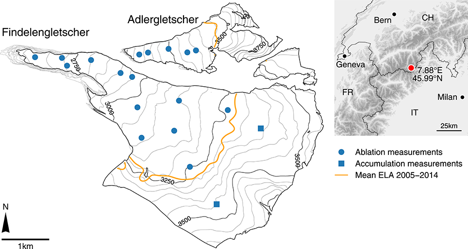
Figure 1. Map of Findelengletscher and Adlergletscher showing the locations of the glaciological mass balance measurements in 2014 as well as the mean equilibrium line altitude (ELA) and the annual glacier outlines for the period studied.

Since the late 1970s, Findelengletscher has been the object of glaciological studies, ranging from glacial hydrology and runoff (Collins, 1979; Iken and Bindschadler, 1986) to the development of methods for mass balance determination (e.g., Machguth et al., 2006a; Huss et al., 2013; Sold et al., 2015). The good availability of ancillary data makes this a suitable site for modeling studies as well as for the validation of new measurement techniques (Joerg et al., 2012; Huss et al., 2014). In 2004, a network of ablation stakes and accumulation measurements was set up, providing the first readings at the end of the hydrological year in 2004/05 (Machguth, 2008; Glaciological Reports, 2011–2015) (Figure 1). In 2009, the goal of the monitoring program was redefined toward establishing a long-term series. Accordingly, the observational network was extended to 11–13 ablation stakes, 1–2 snow density pits and semi-annual measurements (Figure 2). Summer mass balance was obtained around the end of September (Table 1). Ablation stakes consisted of 2 m long PVC tubes which were connected flexibly by short chains. The stakes were placed in the ice by means of a steam drill. When melted out, they were re-positioned to their original location to account for ice flow. Readings were taken as the change in the length of the exposed section. Accumulation was measured at snow pits dug down to a sawdust reference horizon marking the preceding summer surface. The locations of the snow pits were marked permanently by aluminum stakes. The bulk density of snow was determined gravimetrically for each snow pit. Snow probings in the accumulation area were not conducted as part of the summer mass balance surveys because an unambiguous detection of the preceding summer surface in the firn was hampered by melt-refreezing cycles during summer that alter the snow pack structure (Sold et al., 2015).

FIGURE 2

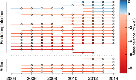
Figure 2. Readings (dots) and measurement periods (lines) of the annual point balance measurements on Findelengletscher and Adlergletscher sorted by elevation such that highest elevation is at the top of the figure.

TABLE 1

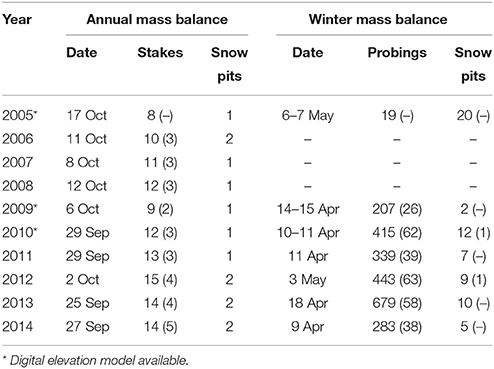
Table 1. Dates of the annual and winter mass balance measurements on Findelengletscher and the respective number of stakes, snow pits, and probings (values for Adlergletscher in parentheses).

Winter mass balance had been measured regularly in April or May since 2009, and consisted of several hundred snow probings and numerous snow density pits at the stake locations across the glacier (Table 1). Two or three snow probings were taken within a few meters' radius to identify and isolate outliers. Snow probings were not performed along a regular grid but followed the paths of the observers while moving from different starting points at the top of the glacier down to the tongue. In the accumulation area the boundary between snow and firn typically was defined by an ice lens that allowed for unambiguous detection by means of a probe.

A smaller measurement program, consisting of 2–5 ablation stakes, was established on Adlergletscher (Figure 1) in 2005. Since then, summer and winter mass balance have been measured in parallel with Findelengletscher.

Ground-penetrating radar (GPR) surveys took place in spring 2012 to 2014 provide snow depth estimates along regular 500 × 500m grid lines covering both glaciers (Sold et al., 2015). In 2005 and 2010 additional surveys were conducted along arbitrary profile lines (Machguth et al., 2006a; Sold et al., 2013). Different systems with central frequencies of 400 and 500 MHz were deployed from a helicopter with a flying speed of 5–20 ms⁻¹ and from about 10 m above the ground. Along with their position in a Differential Global Positioning System, 10 to 50 GPR traces were recorded per second at a sampling interval of 0.20–0.31·10⁻⁹ s (Table 2).

TABLE 2

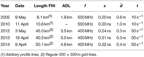
Table 2. Date, length, signal frequency (f), sampling rate (s), average trace spacing ($\overline{d}$), and number of measured traces per second (t) of the GPR measurements of snow accumulation distribution on Findelengletscher (FIN) and Adlergletscher (ADL).

Digital elevation models (DEMs) obtained from airborne laser scanning of the glacier surface are available for autumn 2005, 2009, and 2010. A detailed description of the airborne acquisition, geo-referencing, point cloud interpolation, and generation of the 1 × 1m grid is given by Joerg et al. (2012) together with a detailed uncertainty assessment. For the present study, the DEMs were resampled to 25 × 25m grids.

Glacier outlines were digitized on annual 0.25–0.5 m resolution orthophotos (Swiss Federal Office of Topography). These were not available for the years 2008 and 2011 and the outlines were updated using panchromatic Landsat 7 imagery.

Daily air temperature and precipitation data were obtained from an automatic weather station at Zermatt, located at 1638 m a.s.l., 6 km distance from the glacier tongue. Wind speed and direction were provided by the station at Gornergrat (3129 m a.s.l., 4.7 km distance). Furthermore, daily precipitation, obtained by interpolation of station data to a grid of about 2 km resolution, was available from the RhiresD dataset (MeteoSwiss, 2013). These data were used in only one sensitivity test.

3. Methods

3.1. Glacier-Wide Mass Change from Geodetic Surveys

The geodetic volume change of Findelengletscher was derived for the period 2005–2010 by differencing two LiDAR DEMs (Joerg et al., 2012). The systematic and stochastic uncertainties of the DEMs were assessed thoroughly by Joerg et al. (2012). Whereas, the very high number of measurements on the glacier surface rendered stochastic uncertainties negligible, systematic uncertainties influenced the calculated volume change. Technology-related systematic errors identified by Joerg et al. (2012) canceled out as they were similar in magnitude and direction in both LiDAR data sets. In the following, we (i) corrected the volume change for fresh snow that was present during the LiDAR surveys, (ii) converted volume to mass change, while accounting for (iii) the mass of the fresh snow cover, (iv) the time difference between geodetic and glaciological surveys, and (v) basal and internal mass balance components.

A systematic error in the glacier volume change arose from snowfall events that occurred before both surveys. Distributed measurements of the fresh snow cover by means of snow probings and density pits were used to correct the elevations of the LiDAR DEMs accordingly. In 2005, the in situ measurement campaign took place 12 days before the LiDAR data was acquired. Consequently, the change in snow depth between the two measuring dates had to be corrected as well. By using the available temperature record to roughly estimate melting and compaction during that period, Joerg et al. (2012) derived a mean snow depth of 0.47m at the survey date. In 2010, snow depth measurements were taken on the same day as the LiDAR survey and linear regression of the probings with elevation yielded a mean snow depth of 0.20 m (Joerg et al., 2012). We estimated the related uncertainties in mean snow depth to be ±0.24m and ±0.1m, respectively. The difference in snow volume for the two surveys was subtracted from the total glacier volume change.

To convert volume to mass change, we have evaluated changes in firn thickness and density over time for Findelengletscher according to the method proposed by Huss (2013). By forcing this model with surface mass balance distribution over the last decades (Huss, 2010) and comparing calculated volume and mass change over the 2005–2010 period, we find a bulk volume-to-mass conversion factor of 860kgm⁻³. The uncertainty in bulk density was estimated as ±60kgm⁻³ (Huss, 2013). To subsequently compare the geodetic with the direct glaciological mass balance, the fresh snow cover that was present at the LiDAR survey dates was converted to mass using roughly estimated densities of 270 ± 50kgm⁻³ and 300 ± 50kgm⁻³ for 2005 and 2010, respectively. The time difference of 12 days to the glaciological measurements in 2005 was accounted for by subtracting a mass change of −0.10 m w.e. (water equivalent) in that period, derived by modeling as described below.

To allow for a direct comparison of geodetic and glaciological mass balance measurements, internal and basal ablation and accumulation were subtracted from the total geodetic mass change. This involved (i) internal accumulation by refreezing of meltwater or precipitation below the previous summer surface, because refreezing within the annual accumulation layer was covered by the glaciological measurements; and (ii) basal ablation from the geothermal heat flux and heating by strain and basal friction. Refreezing was assessed by using heat conduction in snow and firn to model end-of-winter temperature profiles (Pfeffer et al., 1991). The one-dimensional model was applied to each grid cell in the accumulation area and for discrete layers of 0.1m thickness. For the sake of simplicity, the available daily air temperature record was used as input. To obtain the depth-dependent thermal conductivity for each grid cell, density was estimated using a simple densification model (Herron and Langway, 1980), coupled with the mass balance model described below. It was calibrated with a set of 19 firn cores from temperate and polythermal mountain glaciers and ice caps in the European Alps, western and Arctic Canada, Central Asia, Patagonia, and Svalbard (Huss, 2013). Because of the temperate nature of Findelengletscher we assumed that subfreezing temperatures were entirely compensated for by refreezing. On the glacier-wide average, refreezing below last year's surface accounts for 0.007 m w.e.a⁻¹. Basal ablation by the geothermal heat flux was calculated using the latent heat of fusion and an estimate of the flux of 0.05 W m⁻² (Medici and Rybach, 1995). Based on typical values for ice thickness, bedrock slope, and flow velocity of Findelengletscher, heating from strain and basal friction was estimated by complete dissipation of the potential energy released by gravitational ice flow. Together these internal and basal processes account for a mass balance of −0.014 m w.e.a⁻¹.

3.2. Glacier-Wide Mass Change from Conventional Glaciological Methods

Point observations of annual ablation were converted to water equivalent using 900kgm⁻³ as the density of ice. The measured densities were used for the accumulation measurements at snow pits. If multiple readings for a snow pit were available, their mean value was taken. The standard deviation from repeat measurements was 21kgm⁻³. The mean density averaged over all years was 501 ± 50kgm⁻³ (n = 14). To obtain winter mass balance, we interpolated density measurements of the individual season to convert probed snow depth to water equivalent. During the 10 year period snow densities showed neither clear spatial or altitudinal trends, nor a robust relation with snow depth. For this reason, the mean density within elevation zones was used.

We applied three common approaches in order to estimate the glacier-wide surface mass balance of Findelengletscher from the annual mass balance measurements: (1) The profile method is based on the assumption that mass balance is a function of elevation alone. We fitted a linear model function to the annual sets of measurements using generalized least squares. In order to derive mass balance at elevations above the uppermost measurements, different elevational gradients were used. Aside from a continuation of the linear model, a constant ceiling value and an inverted gradient were implemented (Escher-Vetter et al., 2009). Application of the model functions to the glacier DEM then provided total mass changes.

(2) The contour line method is based on drawing contours of mass balance, while taking into account the surface mass balance measurements, elevation, terrain characteristics, and expert knowledge such as knowing the position of the snowline (Østrem and Brugman, 1991; Escher-Vetter et al., 2009). We drew contours at 1 m w.e. intervals and mass balance was assumed to be constant within each band. Spatial integration over the surface provided the glacier-wide mass balance. For the balance year 2009/10, a total of 18 repeat evaluations was available that was generated by students in a lab course. This was used to assess a first order estimate of the uncertainty introduced by the manual drawing of contour lines.

(3) Alternatively, we used quadratic inverse distance weighting to interpolate the point observations to the 25 × 25m grid given by the DEMs.

3.3. Glacier-Wide Mass Change from Model-Based Extrapolation

We applied a mass balance modeling scheme to assimilate the full set of seasonal mass balance observations. The numerical model operates at daily time steps, accounting for accumulation and ablation, and has been successfully applied previously to derive glacier mass balance (Huss et al., 2009; Kronenberg et al., 2016). It is described in detail in Huss (2010). The ablation routine is based on a temperature-index approach that additionally accounts for variations in the potential incoming solar radiation (Hock, 1999). Daily melt M is computed as

$\begin{array}{cc}M=\{\begin{array}{l}\left(f_{\text{M}}+r·I\right)T,T\text{ > }0°\text{C}\\ 0,T\le 0°\text{C}\end{array}& (1)\end{array}$

where f_M is a melt factor (md⁻¹K⁻¹), T is air temperature, and I potential solar radiation. A radiation factor r (m³W⁻¹d⁻¹K⁻¹) controls the relative importance of incoming solar radiation compared to the temperature index. It was set separately for snow and ice to account for a different sensitivity to processes that govern surface melt, e.g., due to a different surface albedo. Distributed temperature T was derived from the daily mean air temperature measured in Zermatt, which was first extrapolated to the median glacier elevation using monthly temperature gradients derived from surrounding meteorological stations and was then distributed across the glacier surface using a lapse rate dT/dz. Surface elevation was taken from the most recent DEM of 2005, 2009, or 2010.

Measured precipitation P was scaled by a correction factor c_prec to account for systematic under-catch of the station (e.g., Neff, 1977) and its location at the valley bottom at 1638 m a.s.l.. A threshold of T = 1.5°C with a linear transition range of the rain-snow fraction between 0.5 and 2.5°C separated solid from liquid precipitation (Hock, 1999). To derive accumulation, solid precipitation was distributed using a spatial snow distribution multiplier D_snow (Tarboton et al., 1995; Farinotti et al., 2010):

$\begin{array}{cc}\begin{array}{l}C(x_0,t)=P(t)·c_{prec}·D_{snow}(x_0),\hfill \end{array}& (2)\end{array}$

where C is accumulation at location x₀ and time t. The sum of accumulation and melt provided the evolution of the snow cover that was used to set the glacier surface type (ice / snow). In order to derive realistic accumulation patterns, the interpolated snow depth distribution, normalized to a mean value of 1, was used as the multiplier D_snow. Thus, measured snow depth was not a direct input variable to the model but served as reference for the calibration of the precipitation correction. If D_snow was set accordingly, point observations of winter mass balance were matched exactly, despite small amounts of melting during the winter that alter modeled accumulation. In this study we ran the model using various realizations of snow accumulation distribution based on different sets of point observations (see below). For years with no observations available (2006–2008) a mean normalized distribution was used, scaled by a non-calibrated prescribed precipitation correction c_prec.

We aimed at calibrating the model with all available measurements to obtain a consistent and homogeneous time series of mass balance for the period 2004/05 to 2013/14. The parameter values to define were f_M, r_snow, r_ice, c_prec, and dT/dz. In years with observations of snow accumulation, c_prec was chosen so that the modeled winter accumulation at the measurement locations matched the observations. Then f_M, r_snow, and r_ice were adjusted iteratively by minimizing the root-mean-square error (RMSE) with in situ observations of annual mass balance while keeping their proportions constant. However, a straightforward calibration of the remaining parameters and proportions is difficult and not robust because the parameters counteract each other. Most importantly, changes in the temperature lapse rate can be countered by a different ratio of r_snow and r_ice, while their absolute value could to some degree compensate for changes in f_M. Thus, minimum RMSEs could be achieved with a variety of parameter combinations that can be outside a physically reasonable range and yield different mass balance estimates. By additionally considering surface characteristics at the stake locations and their distribution across the glacier, we manually adjusted the following parameters on an annual basis in order to obtain an optimal fit to the in situ mass balance measurements: dT/dz, the ratios r_snow/r_ice and r_ice/f_M, and c_prec in years without snow accumulation measurements.

3.4. Seasonal Accumulation Measurements from Helicopter-Borne GPR

Internal reflection horizons (IRH) in GPR data are induced at boundaries in dielectric material properties (Ulriksen, 1982). In the context of accumulation measurements, such changes are driven by contrasting material densities between snow, firn, and ice (Plewes and Hubbard, 2001). To extract snow depth from airborne GPR data we aimed at locating the IRHs corresponding to the snow surface, the snow-ice, or the snow-firn boundary. To reduce noise and to improve the contrast of IRHs, numerous processing techniques have been developed, many of which are inherited from different geophysical methods such as seismic reflection surveys (Daniels, 2004). However, no universally valid processing scheme exists, as the characteristics of GPR data strongly depend on the survey design and the properties of the subsurface material (Ulriksen, 1982). Here we applied a scheme that was previously used to process airborne GPR data in the context of snow depth measurements (Sold et al., 2013). The scheme consists of a frequency bandpass filter, background removal, gain function, and spatial interpolation to match the mean trace spacing and to account for variations in the flying speed of the helicopter. The IRH corresponding to the snow surface could then be digitized semi-automatically using a phase-following tool in the processing software (Reflexw, Sandmeier Scientific Software). In the ablation area the bottom of the snow pack was represented by a pronounced change in density at the snow-ice boundary, generating a strong IRH. In the accumulation area, however, the contrast in the densities of snow and underlying firn was smaller and multiple layers of firn were detected (Sold et al., 2015). Thus, a careful interpretation of the GPR data was required to avoid misinterpretation of IRHs. The bottom of the snow pack was digitized manually, as the roughness of the underlying ice or firn surface impeded semi-automatic tracking.

The difference in GPR signal travel time between the IRH of the snow surface and the lower boundary could not be extracted from about 10 % of total measured data, mostly due to crevasses. The travel time was converted to depth using an empirical relation with dry-snow density (Frolov and Macheret, 1999). In line with the conventional glaciological measurements of winter mass balance, the elevation-zone based extrapolation of snow density was used. While doing this, we assumed liquid water within the snow pack to be negligible. This is supported by direct observations in the snow density pits and sporadic temperature measurements at the pit walls in spring 2013 and 2014 that, aside from the uppermost centimeters, generally revealed subfreezing snow temperatures with exception of the lowermost ~10 % of the glacier surface (see Section 5.4).

3.5. Generalizing Snow Accumulation Distribution

We derived a set of snow accumulation grids from the available measurements to constrain accumulation in the mass balance model. This involved annual grids for D_snow (Equation 2) obtained from (i) the conventional annual snow probings in spring 2009–2014 and (ii) the GPR measurements in spring 2012–2014.

The snow probings taken during winter surveys were interpolated using inverse-distance weighting with a search radius of 400 m. If the search radius contained less than three measurements, it was increased stepwise until a sufficient number of points was reached. Small-scale variability was overlain using an index based on curvature evaluated within a radius of 150 m around each grid cell. Cells with concave (convex) surfaces were attributed higher (lower) accumulation using a linear relation with curvature. Furthermore, snow depth was decreased linearly for steep slopes of between 40 and 60°, and was set at zero above the latter threshold (Huss et al., 2008). Though they were minimal across most of the glacier surface, these adjustments were important for yielding realistic snow depths in regions prone to avalanching and wind erosion.

The GPR measurements provided snow accumulation along linear profiles of about 500 m spacing. Along the profiles, however, the spatial resolution was higher and an interpolation scheme should be able to utilize this information to fill the gaps between profiles. Because snow accumulation reveals trends in the mean accumulation, e.g., with elevation, and differences in the variability, such as through higher wind speeds at higher elevations (Helfricht et al., 2014), it must be considered a non-stationary process. To take this into account we applied geographically weighted regression (GWR) that allowed for spatial variations in the influence of the explaining variables (Brunsdon et al., 1996; Fotheringham et al., 1998). To avoid effects of subgrid variability, GPR measurements were aggregated to a 25 m spacing beforehand. The interpolation was applied after conversion from snow depth to water equivalent using the interpolated measured densities. For a given location x₀, the snow accumulation s was derived by multiple linear regression with independent variables c_i so that

$\begin{array}{cc}s(x_0)={\beta }_0(x_0)+{\displaystyle \sum _{i=1}^n{\beta }_i}(x_0)·c_i(x_0),& (3)\end{array}$

where n is the number of independent variables. The regression coefficients β_{0, …, n} were estimated for each location x₀ by least squares from the set of weighted GPR measurements. The weights were obtained from a Gaussian weighting function as

$\begin{array}{cc}\begin{array}{l}{w}_j(x_0)=\text{exp}(-d{(x_0,x_j)}^2·l^{-2}),\hfill \end{array}& (4)\end{array}$

where 0 < w_j ≤ 1 are the weights of the j = 1, …, m GPR measurements, d the distance function and l a range parameter. Observations where $d>\sqrt{3.0·l^2}$ and, thus, w_j < 0.05 were omitted. Elevation was chosen as an independent variable in order to respect the general altitudinal trend. In addition, we tested the interpolation performance using several terrain-based indices as a second independent variable. This comprised (1) curvature, computed following Zevenbergen and Thorne (1987). Different spatial “scales” (25 m, 50 m, 75 m, 125 m, 250 m) of curvature were obtained by scaling of the 3 × 3 kernel (i.e., 25 m scale) to the respective size on the 25 × 25m DEM grid. (2) A high-pass filter, implemented on the same set of scales by subtracting the Gaussian-weighted (Equation 4) kernel average from the DEM. (3) Winstral's S_x (Winstral et al., 2002) was derived with a maximum search radius of 1000 m for the main wind direction (SE), measured at the Gornergrat weather station. (4) Positive and (5) negative openness (Yokoyama et al., 2002) were calculated as the mean of 12 equally wide directional sectors and maximum distance of 1000 m. Each terrain index was tested on the annual sets of measurements with different settings for the range parameter l of 500m, 1000m, 1500m, 2000m, 2500m (Equation 4). The smallest average RMSE to the snow probings was found as 0.28 m w.e. for the regression setup with elevation and 125 m scale curvature and a range parameter of l = 1000m. For the years where GPR measurements were performed along regular grid lines (2012, 2013, and 2014) this configuration was applied to derive the annual snow accumulation pattern. After normalizing the extrapolated accumulation distribution to an average value of 1 over the glacier surface, the grids were used as D_snow in Equation 2. For the remaining years, the 3 year mean of the normalized annual grids was computed, which can be scaled by the independent c_prec in the mass balance evaluation scheme (Equation 2).

As an alternative to the regression approach presented here and in order to assess the sensitivity of mass balance evaluation schemes to the interpolation method, we used inverse-distance weighting to derive a smooth and topographically independent grid of snow accumulation. As before, Equation 4 with l = 1000 m was used for the computation of weights and a mean normalized distribution grid was generated for years in which no extensive GPR measurements were available.

4. Results

4.1. Glacier-Wide Mass Balance

The geodetic mass change for the period 2005–2010 revealed a pronounced mass loss of −2.86 ± 0.25 m w.e. and −1.62 ± 0.19 m w.e. for Findelengletscher and Adlergletscher, respectively. Note that these results varied slightly from Joerg et al. (2012) because of differences in the glacier outlines used for calculating glacier-wide averages. The reported uncertainty accounts for snow cover that was present during the Lidar surveys in 2005 and 2010, and for the density used to convert volume to mass change. For all values reported below, the estimated basal and internal balances were subtracted from the total mass change in order to allow for comparison with measurements of surface mass balance. For Findelengletscher and Adlergletscher, this yielded a mean annual surface mass balance of −0.59 m w.e.a⁻¹ and −0.34 m w.e.a⁻¹ for the mass balance years 2005/06 to 2009/10.

The point measurements of annual mass balance (Figure 2) showed a clear trend with altitude that was used to extrapolate the measurements to the entire glacier (profile method). Linear regression with elevation for each year performed excellently with a mean of R² = 0.97 ± 0.02 (p < 0.01) (Figure 3). For 2005/06 to 2009/10, corresponding to the period covered by the geodetic surveys, mean mass balance is +0.39 m w.e.a⁻¹. Maximum balances at highest elevations of more than +7 m w.e.a⁻¹ (2008/09) are likely unrealistic, but cannot be verified as no direct observations are available. The elevational trends are dominated by ablation and, hence, by the temperature lapse rate. Accumulation processes, by contrast, do not necessarily follow these altitudinal trends and are underrepresented in the regression. This can be accounted for by using cut-off values or inverting the elevational trend above a threshold elevation (Escher-Vetter et al., 2009). Here we assumed (i) constant mass balance or (ii) decreasing balance at elevations above 3460 m a.s.l., i.e., the elevation of the uppermost point observation (Figure 3). By affecting 28 % of the glacier surface, this yielded average mass balances of (i) +0.06 m w.e.a⁻¹ and (ii) −0.08 m w.e.a⁻¹, which is substantially more positive than the geodetic method (Figure 4).

FIGURE 3

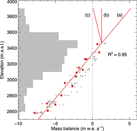
Figure 3. Elevation distribution of mass balance measurements on Findelengletscher in 2012 (red dots) and all other years (gray dots). Red lines show model functions of elevation used for the profile method and (a) linear, (b) constant, and (c) inverted gradients above 3460 m a.s.l.. Gray horizontal bars show the area-elevation distribution of Findelengletscher.

FIGURE 4

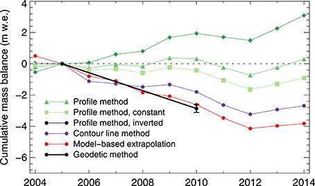
Figure 4. Cumulative mass balance of Findelengletscher 2004–2014 obtained from the profile method (green), with a linear gradient for the entire glacier surface, constant accumulation above 3460 m a.s.l., and an inverted elevational trend above the same elevation; (violet) the contour method; (red) the model-based extrapolation scheme; (black) the geodetic mass change that is given as reference. Note that the geodetic mass change covers the period 2005–2010 and, for visualization, balance series were aligned by the 2005 data points. Results from the inverse distance weighted interpolation (IDW) of observations are not shown because they are outside the plot range (−12.2 m w.e. for 2005–2014).

The contour line method takes into account expert knowledge to achieve reasonable patterns of mass balance. The resulting glacier-wide surface mass balance of −0.36 m w.e.a⁻¹ (2005/06 to 2009/10) agrees better with the geodetic mass change than the profile method, but likewise shows a positive bias. The set of 18 repeat evaluations for the 2009/10 balance year (Section 3.2) yielded a standard deviation of 0.17 m w.e., which can be considered a rough estimate for the uncertainty arising from subjectivity in the interpretation.

Attempts to use spatial interpolation approaches that do not explicitly take into account the elevational trend in mass balance observations did not generate reasonable results. Quadratic inverse distance weighting converges to the mean value for large distances from observations, and thus generated positive mass balance only in the immediate vicinity of the sparse accumulation measurements. Because this method yielded an unrealistically strong negative mass balance of −1.64 m w.e.a⁻¹ on average for the period covered by the geodetic mass change, the results are not discussed in further detail.

The mass balance model (Section 3.3) was calibrated as described above, using the complete set of seasonal glaciological measurements and the snow accumulation data from GPR (Table 3). The mean RMSE with annual point mass balance observations over the 10 year period was 0.41 m w.e., ranging from 0.27 to 0.60 m w.e. for individual years. Starting at the date of the annual measurements, the model computed the daily evolution of mass balance for each 25 × 25m grid cell (Figure 5). This also allowed for temporal homogenization of the results to, e.g., the hydrological year.

TABLE 3

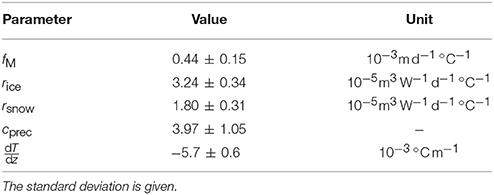
Table 3. Average of calibrated model parameters over the 10 year study period.

FIGURE 5

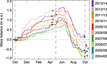
Figure 5. Calculated daily evolution of glacier-wide mass balance for all years analyzed. Dots show the dates of measurements (Table 1), and vertical stippled lines mark the summer and winter seasons according to the hydrologic year.

The model generated plausible maps of glacier surface mass balance distribution by taking into account the major processes that govern spatial variation in snow and ice ablation (Supplementary Material), including an adequate representation of snow accumulation distribution based on the GPR snow measurements (Figure 6A). Below 3500 m a.s.l. mass balance increases more or less linearly with elevation, but does not show a clear trend at higher altitudes (Figure 6B). The spatial pattern of mass balance was rather consistent over the 10 year period, with the largest deviations from the annual mean balance occurring in the upper accumulation area and on the glacier tongue. For 84% of the glacier area, the range was less than 1 m w.e.a⁻¹, while it was more than 2 m w.e.a⁻¹ for 2% of the area.

FIGURE 6

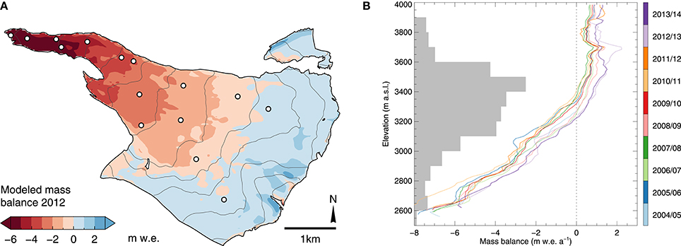
Figure 6. (A) Map of glacier surface mass balance 2011/12 derived from model-based extrapolation of observations; dots show the locations of the respective point balance observations; gray lines are 100m elevation contours. (B) Vertical gradients in annual glacier mass balance derived from model-based extrapolation in 2004/05 to 2013/14. Gray horizontal bars show the area-elevation distribution of Findelengletscher.

The mass balance of Adlergletscher was evaluated in the same way as for Findelengletscher, but starting with the later onset of measurements in 2005. Both time series revealed a negative balance for the study period prior to 2012 and a slight mass gain in 2013 and 2014 (Figure 7). This is in line with the annual in situ observations that yielded increased winter accumulation for these 2 years (Figure 2). For Findelengletscher, annual mass balance was −0.52 m w.e.a⁻¹ on average for the period covered by the geodetic mass change (Figure 4). Mean winter and summer balance was +0.87 m w.e.a⁻¹ and −1.39 m w.e.a⁻¹, respectively. Adlergletscher had a lower winter balance of +0.62 m w.e.a⁻¹ but a less negative summer balance (−0.96 m w.e.a⁻¹). This resulted in a mean mass balance of Adlergletscher for 2005/06 to 2009/10 of −0.35 m w.e.a⁻¹, substantially less negative than for Findelengletscher (Table 4).

FIGURE 7

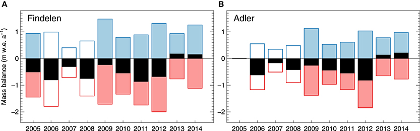
Figure 7. Evaluation of summer (red), winter (blue), and annual (black) mass balance of (A) Findelengletscher and (B) Adlergletscher based on the model-based extrapolation approach. Unfilled bars indicate mass balances that were not constrained by observations of winter snow accumulation.

TABLE 4

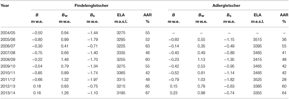
Table 4. Annual (B), winter (B_w) and summer (B_s) surface mass balance, equilibrium line altitude (ELA), and accumulation area ratio (AAR) of Findelengletscher and Adlergletscher derived by model-based extrapolation of seasonal observations in 2005 to 2014.

4.2. Snow Accumulation Distribution

Snow accumulation distribution showed a clear overall elevational trend with maximum values in the northern and south-western accumulation area (Figure 8A). Higher variability in accumulation was found at higher elevations. The mean normalized accumulation distribution for 2012–2014 was used to compute the winter mass balance for the years with no available GPR surveys. Over the 3 year period, the general accumulation patterns were similar. For 86% of the glacier area, the range in accumulation was less than 25% of the average normalized accumulation pattern in 2012–2014 (Figure 9). In contrast, considerable differences exist in the small-scale pattern for some areas, in particular at high elevations: for 1% of the area, the range was over 100% of the average normalized accumulation.

FIGURE 8

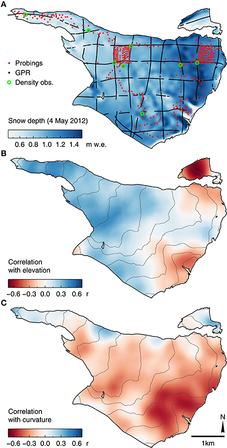
Figure 8. (A) Snow accumulation distribution on 4 May 2012 derived from the GPR measurements by GWR interpolation. Correlations of snow depth with (B) elevation and (C) curvature (125m scale). Gray lines in (B,C) are 100m elevation contours.

FIGURE 9

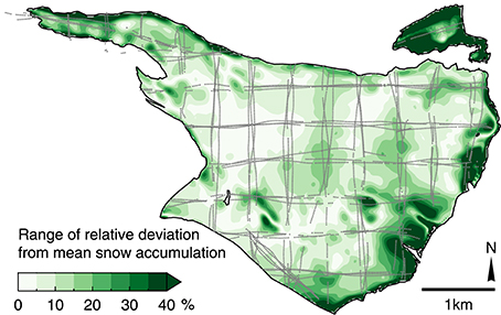
Figure 9. Temporal variability of the snow accumulation pattern shown as the range of the relative deviation (in %) from the normalized snow accumulation distribution averaged over 2012–2014. Gray dots show GPR measurements of the same period.

For the years where extensive GPR surveys were available, the snow accumulation distribution was derived using GWR interpolation with elevation and 125m-scale curvature as independent variables. The correlation of snow depth with elevation was positive for low and mid-elevations on the glacier, but changed sign at high elevations in the accumulation area (−0.70 < r < 0.50, Figure 8B). For curvature, correlations were generally lower (|r| < 0.60) and showed considerable spatial variations. While the higher variability of accumulation at high elevations was reproduced, correlations shifted to counter-intuitive positive values for several smaller areas near the glacier margin (Figure 8C). The mean performance of the interpolation scheme over the entire glacier area was R² = 0.37 ± 0.12.

5. Discussion

5.1. Uncertainties in Mass Balance Evaluations

We follow previous studies to estimate the uncertainties inherent to the evaluation of glacier-wide surface mass balance (Thibert et al., 2008; Huss et al., 2009; Zemp et al., 2013). Point balance measurements are prone to errors in stake readings and the subsequent mass conversion. We roughly estimate the combined random uncertainty to be 0.1 m w.e. and 0.3 m w.e. per reading in the ablation and accumulation areas, respectively (Huss et al., 2009). Assuming the errors to be independent for the measurement network on Findelengletscher, the uncertainty in the mean of all point balances reduces to an annual average of 0.04 m w.e.. Errors due to changes in glacier extent (Koblet et al., 2010) are minimized by updating the glacier outlines on an annual basis.

To obtain glacier-wide surface mass balance using the profile method, an uncertainty estimate was derived from the one-sigma confidence intervals of the regression coefficients. This yielded an average uncertainty of 0.11 m w.e.a⁻¹, depending on the number of observations in the annual subsets. Note that this does not include potential gross errors related to the balance gradient assumed in the accumulation zone.

Uncertainty in the contour line method is owed mainly to subjectivity in interpretation and manual drawing of contours, and was assessed through 18 independent evaluations of the 2009/10 point observations by different observers. The standard deviation in glacier-wide mass balance was 0.17 m w.e.a⁻¹, and is assumed to be of similar magnitude for the remaining years.

The uncertainty in the model-based extrapolation of mass balance was estimated by altering the model parameters which are not directly constrained by observations. The intervals were prescribed as −0.7 ≤ dT/dz ≤ −0.5·10⁻³°Cm⁻¹ for the temperature lapse rate, 0.5 ≤ r_snow/r_ice ≤ 0.8 as the ratio of the radiation factors, and a value of $1.2\le r_{\text{ice}}/f_{\text{M}}\le 12.0·10^{-2}{m}^2{W}^{-1}$ to describe the relative importance of r_ice to the melt factor f_M (Equation 1). The setup of varying ratios was chosen instead of altering absolute values in order to obtain realistic parameter combinations. For n = 7³ model runs, the parameters were varied uniformly within the specified intervals and the resulting standard deviation of 0.13 m w.e.a⁻¹ provided an estimate of the uncertainty in the model-based extrapolation of point balance observations.

5.2. Re-Analysis of Mass Balance Series

We have re-analyzed a mass balance series using a set of different evaluation schemes. All schemes make use of the glaciological point balance observations to derive glacier-wide mass balance, while only the model-based extrapolation also integrates measurements of winter mass balance. The approaches are compared to the geodetic mass balance, which serves as a reference for the period 2005–2010. As described above, to allow for a direct comparison, internal and basal balance components were subtracted from the geodetic mass change. We follow Zemp et al. (2013) to examine the consistency of the mass balance series with the geodetic mass change. They calculate the reduced discrepancy δ as

$\begin{array}{cc}\begin{array}{l}{\delta }_i=\frac{B_i-B_{\text{geod}}}{\sqrt{{\sigma }_i^2+{\sigma }_{\text{geod}}^2}},\hfill \end{array}& (5)\end{array}$

where B_i and B_geod are the cumulative mass balances for the period 2005/06 to 2009/10 calculated with the respective evaluation scheme (i) and the geodetic mass balance, respectively, and σ_i and σ_geod are the random errors. Based on the independence of the error sources, σ_i is the combined error of the evaluation scheme itself and the error in point balance observations. Thus, δ can be assumed to follow a normal distribution with unit variance (Zemp et al., 2013). This allows testing for a significant difference between the cumulative balances as the alternative hypothesis. If δ is within the the 95 % confidence interval (|δ| < 1.96) the null hypothesis is not rejected and the two time series can be assumed to agree within their uncertainty bounds.

The profile method, in its simplest form, linearly extrapolates the strong elevational trend of observations in the ablation area to the entire glacier surface (Figure 3), which leads to a pronounced glacier mass gain. More realistic values were obtained when altering the gradient at higher elevations (Escher-Vetter et al., 2009). Although a constant and an inverted elevational gradient above 3460 m a.s.l. generate a lower mass balance, all three approaches to implementing the profile method reveal a substantial positive deviation from the geodetic mass change of +0.96 m w.e.a⁻¹ (linear), +0.64 m w.e.a⁻¹ (constant above 3460 m a.s.l.), and +0.49 m w.e.a⁻¹ (inverted). These differences and the uncertainties reported above yield 6.54 ≤ δ ≤ 12.86 with p < 0.01 and, thus, significant deviations from the geodetic mass change for all three implementations of the profile method.

The contour line method results in a mass balance time series that reflects the observed volume change. However, compared to the geodetic mass change, the balance series is 0.21 m w.e.a⁻¹ more positive (Figure 4). With the uncertainty obtained from repeat evaluations and errors in point balances, this deviation is significant with δ = 6.19 and p < 0.01.

For the presented model-based evaluation approach, the deviation from the geodetic mass balance for the period 2005/06 to 2009/10 is 0.04 m w.e.a⁻¹ and −0.04 m w.e.a⁻¹ for Findelengletscher and Adlergletscher, respectively. For Findelengletscher, the balances and uncertainties reported above yield δ = 0.48, which is within the 95 % confidence interval and corresponds to p = 0.63. Thus, the null hypothesis is not rejected and the two time series can be assumed to agree within their uncertainty bounds. This similarly holds true for Adlergletscher. For both glaciers, a further conciliation, such as a subsequent calibration of the glaciological series (e.g., Hagg et al., 2004; Huss et al., 2009), is not required. We conclude that, in contrast to the profile or contour line method, the model-based extrapolation reliably reproduces the annual surface mass balance. This can be attributed to the adequate representation of the accumulation distribution by assimilation of all available data in the model. In this context, the ability to integrate end-of-winter measurements of snow accumulation is particularly advantageous, as they can be obtained more efficiently than observations of annual accumulation and ablation at the end of summer, and they contain considerable information on spatial mass balance variability. The mass balance time series presented in Figure 7 is, thus, reported as being the optimal result of the re-analyzed measurement series.

Although the presented approaches for deriving glacier-wide surface mass balance show a large spread in the cumulative mass change over the 10 year period (Figure 4), they reveal considerable agreement in the temporal variability of mass balance. Using the model-based extrapolation as reference for a correlation analysis, the contour method reveals r = 0.85. For the profile method with the linear model function, correlation is r = 0.86. Highest correlation of r = 0.93 was found for the interpolation of observations by inverse-distance weighting (p < 0.01 for all given correlations).

5.3. The Benefits of Extensive Snow Accumulation Measurements

In this study, airborne GPR surveys provided abundant accumulation measurements. The good agreement of the model-based extrapolation approach with the geodetic mass change (Figure 10) indicates that the accumulation distributions derived from interpolation of GPR measurements are appropriate. However, extensive GPR measurements are seldom available. We therefore examined the benefits obtained from the GPR measurements by evaluating the mass balance using a variety of scenarios on snow accumulation data availability. These were the cases where (a) no snow accumulation observations were conducted; and (b) where only the conventional winter mass balance measurements from snow probings and density pits were available. Because GPR measurements were conducted for 3 years and the mean normalized accumulation pattern was applied in the remaining years, we also tested scenarios (c) where this universal pattern was derived from one individual GPR survey only. An additional scenario (d) aimed at investigating the effect of using different interpolation schemes to derive distributed accumulation from GPR measurements (Section 5.4).

FIGURE 10

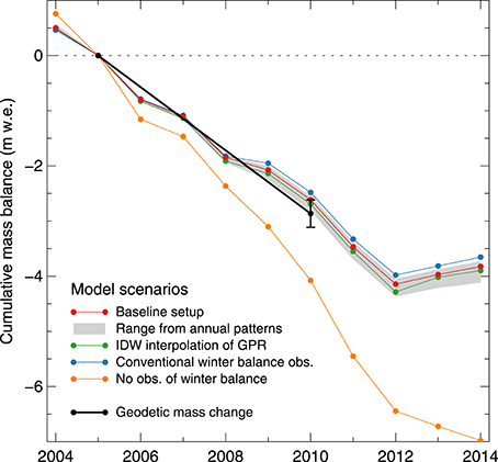
Figure 10. Cumulative mass balance of Findelengletscher for 2004/05 to 2013/2014 obtained from different model setups of snow accumulation: (red) using the GWR-interpolated GPR measurements (baseline scenario) as in Figure 4; (gray) range resulting from using the individual GPR measurements of 1 year for the entire period; (green) using inverse-distance weighting (IDW) for interpolation of GPR measurements; (blue) with conventional winter balance measurements by means of snow probings and density pits; and (orange) with no observations of winter mass balance available and the application of an altitudinal precipitation gradient and fixed precipitation correction instead. The geodetic mass change (black) is given and covers the 2005–2010 period. For visualization, balance series were aligned by the 2005 data points.

If no winter mass balance measurements were available (Scenario a), the precipitation correction c_prec could not be calibrated and an alternative D_snow had to be defined (Equation 2). In this case, the model only used the annual mass balance measurements for calibration and fell back on prescribed values for the precipitation correction and an altitudinal precipitation gradient. Then D_snow was calculated as

$\begin{array}{cc}\begin{array}{l}{D}_{\text{snow}}(x_0)=g_{\text{prec}}·(z(x_0)-z_{\text{med}}),\hfill \end{array}& (6)\end{array}$

where g_prec describes the relative change in precipitation with elevation, z(x₀) the elevation at location x₀, and z_med the glacier median elevation. To examine whether accumulation could be estimated adequately from daily gridded precipitation data, c_prec and g_prec were adopted from 24 grid points of the RhiresD dataset in the vicinity of Findelengletscher (c_prec = 2.04, $g_{\text{prec}}=4.24·10^{-4}{m}^{-1}$). This provided a rough estimate of accumulation and yielded a mean mass balance of −0.82 m w.e.a⁻¹ for 2005/06 to 2009/10. This value was considerably more negative as compared with the geodetic reference or the baseline scenario of using the GPR-derived snow accumulation (Figure 10). Furthermore, this weak representation of the snow accumulation pattern reduced the ability of the model to reproduce the in situ observations of mass balance. The mean RMSE with annual point balance observations increased significantly to 0.79 m w.e. with respect to the baseline scenario (p < 0.01, paired t-test).

If conventional snow probings were available (Scenario b) an arbitrary setting of the precipitation correction and gradient could be avoided. Accumulation was then obtained for every grid cell using the default interpolation scheme based on an inverse-distance approach. However, no winter mass balance measurements were available for the years 2006–2008 and so the mean normalized distribution from the probings in the remaining years was used. The resulting mean mass balance for 2005/06 to 2009/10 deviated from the geodetic reference by +0.08 m w.e.a⁻¹ (Figure 10). The use of snow probings yielded a better model performance than the precipitation gradient Scenario (a). The RMSE relating to annual point mass balances of 0.42 m w.e. was significantly lower (p < 0.01, paired t-test). No considerable difference in the RMSEs was found compared to the scenario with GPR-based snow accumulation distribution because snow probings were taken at most of the mass balance stake locations used for the computation of RMSEs (p = 0.39, paired t-test). In order to assess the benefit of the extensive winter mass balance measurements by means of helicopter-borne GPR (baseline scenario) over the set of conventional observations from probings (Scenario b), a cross-validation of the two datasets was performed: Each GPR dataset from 2012 to 2014 was split in a training and validation set. To account for the neither uniform nor random distribution of GPR observations, they were split by the direction of profile lines into a meridional and a zonal subset of about equal size. Interpolation by GWR was performed on each training subset as described above. The interpolated training sets were then compared to the observations in the validation sets. On average for the 3 years, RMSE was 0.30 m w.e. of snow accumulation when the zonal subsets were used for validation, and 0.31 m w.e. for the opposite choice. Then the interpolated sets of snow probings were used as the training sets. Average RMSE with the validation sets was 0.31 m w.e. and 0.34 m w.e. for the zonal and meridional validation sets, respectively. This could be attributed to the reduced spatial coverage of the glacier by the available probings as opposed to the subsets of GPR measurements.

To estimate the distribution in years when only probings or no in situ observations were available, a mean accumulation pattern was computed from the GPR accumulation measurements of 3 years. This approach is sensitive to potential variations in the accumulation pattern that are driven by interaction of precipitation, wind, and topography (Deems et al., 2008; Schirmer and Lehning, 2011; van Pelt et al., 2014). For Findelengletscher, the data basis does not allow for a full assessment of the uncertainties introduced by this simplification. Instead, in Scenario (c), we used the three measured accumulation patterns individually to obtain the accumulation distribution for the entire 10 year period in order to quantify the effect of variations in the accumulation patterns on the glacier-wide mass balance. The resulting time series deviated from the baseline scenario by −0.03 to +0.01 m w.e.a⁻¹ (Figure 10). The 10 year mean model performance in reproducing annual point balance observations (RMSE) ranged from 0.40 to 0.45 m w.e. for the three realizations of accumulation distribution. However, for the 3 years in which the respective GPR surveys were conducted, the annual RMSE increased marginally (< 0.01 m w.e.). Thus, the effect of using accumulation patterns derived for individual seasons is minimal, and the use of the mean accumulation pattern, in the case of Findelengletscher, was not likely to introduce major uncertainties.

5.4. Uncertainties in GPR-derived Snow Accumulation Distribution

Travel time of the GPR signal from the snow surface to the snow–ice or snow–firn boundary was converted to depth using an empirical relation with snow density (Frolov and Macheret, 1999) that is also used to convert snow depth to water equivalent. Thus, uncertainties in the density measurements and their extrapolation affect the GPR-derived snow depth and the mass balance computations. The GPR signal velocity can be altered further by liquid water present within the snow cover (Schmid et al., 2014). As compared to dry snow, a hypothetical volumetric water content of 5% reduces the GPR signal velocity by about 20% (Frolov and Macheret, 1999). In this study, the GPR surveys were conducted in spring when air temperatures were still low and little melting had occurred. Sporadic measurements of temperature were conducted in the snow pits during the winter mass balance campaigns in 2013 and 2014. While they reveal subfreezing temperatures for most of the glacier area, the uppermost decimeters of the snow pack were isothermal on the lower glacier tongue. Thus, the presence of liquid water has a potential effect on the GPR-derived snow depth at lower altitudes. A comparison at elevations below 3000 m a.s.l. provides evidence of a potential overestimation of the GPR signal velocity for the survey on 3 May 2012. The mean measured snow accumulation by GPR was 0.88 ± 0.23 m w.e. (n = 174) and, thus, significantly higher (p < 0.01) than 0.70 ± 0.28 m w.e. (n = 54) by snow probings. However, in 2013 and 2014, when surveys were conducted earlier in the season, no clear deviation was found (p = 0.70, p = 0.60) and thus the effect on the re-analyzed mass balance time series is likely to be small.

To assess the effect of using different interpolation schemes to derive the accumulation grid from the GPR measurements, the 10 year analysis was run in Scenario (d) where the snow accumulation distribution grid was derived by inverse-distance weighting. A Gaussian weighting curve with a range parameter of l = 1000m (Equation 4) was used, generating a smooth distribution. As for the baseline setup with GWR interpolated, GPR-derived snow accumulation, the mean grid of 2012–2014 was used in the remaining years. This had a very limited effect on the resulting mass balance (Figure 10). RMSEs did not differ significantly from the baseline setup (p = 0.12, paired t-test). This also held true if the annual smooth snow accumulation distribution in 2012–2014 was also replaced by the mean grid. Thus, the evaluation scheme was rather insensitive to whether the small-scale distribution of snow accumulation was resolved. As shown above, the limited spatial coverage of the glacier by the set of snow probings, in contrast, led to a poor representation of snow depth in unmeasured areas and a considerable deviation in the model-derived mass balance.

6. Conclusions

We presented a mass balance time series re-analysis of Findelengletscher and Adlergletscher using a variety of interpolation approaches. Glaciological point measurements of annual mass balance were evaluated using the profile method and the contour line method. Compared to the geodetic mass balance over a 5 year period, the profile method yielded mass balances that were too positive by 0.49–0.96 m w.e.a⁻¹, depending on the elevational gradient used at highest elevations. The contour method agreed more with the geodetic reference, but still deviated considerably (+0.21 m w.e.a⁻¹). We attribute this bias to the sparsity of observations at high elevations. From the given set of measurement locations, the evaluation schemes were not capable of adequately estimating accumulation in unmeasured areas. This held true also for a simple spatial interpolation by inverse-distance weighting which tended to underestimate accumulation for large areas and to generate a time series that deviated strongly from the geodetic reference.

For both glaciers, extensive winter accumulation measurements were available from snow probings and helicopter-borne GPR. In order to assimilate the complete set of seasonal observations, these measurements were used to constrain a distributed mass balance model. For the 10 year period, this model-based mass balance extrapolation yielded a substantial cumulative mass loss at Findelengletscher of −4.34 m w.e.. Adlergletscher, located in a drier setting than Findelengletscher, revealed a mass balance that was, on average, 0.12 m w.e.a⁻¹ more positive. For both glaciers, the model-based evaluation was within the error bounds of the geodetic mass change. By comparing different scenarios on the availability of winter accumulation measurements, it was shown that this excellent agreement was owed to an adequate representation of winter accumulation distribution. If no measurements of snow accumulation is available, accumulation is often estimated by applying altitudinal precipitation gradients. In the case of Findelengletscher, such a simplified description of accumulation yielded a considerably different mass balance series (−0.24 m w.e.a⁻¹ difference) along with the significantly reduced ability of the model to reproduce annual point balance observations.

If the model-based extrapolation was run using the accumulation patterns derived from observations by snow probings and density pits, the balance series was 0.08 m w.e.a⁻¹ more positive than the geodetic method. Although it provided a substantial improvement over using no winter accumulation data, the calculated mass balance was outside the uncertainty range of the geodetic method. Hence, for all presented evaluation approaches, the model-based extrapolation with winter accumulation measurements from helicopter-borne GPR was the only setup that matched the geodetic mass change.

In this study, helicopter-borne GPR measurements in spring 2012 to 2014 provided a mean normalized accumulation distribution that was applied to the years where no extensive accumulation observations were available. It was shown that the general pattern of accumulation was consistent for the short period of 3 years. Future investigations and a larger data basis are necessary to quantify the uncertainty introduced by this simplification. However, the presented results indicate that extensive snow accumulation measurements are beneficial to mass balance evaluations even when they were not obtained for the complete study period. The re-analyzed mass balance series of Findelengletscher and Adlergletscher provide a reference for future studies. Thus, it is essential to continue this monitoring program, along with additional geodetic surveys and measurements of winter accumulation.

Author Contributions

LS wrote the manuscript and evaluated the GPR data; MHu contributed the modeling scheme; HM provided measured data; PJ and MZ evaluated the geodetic mass change; HM, GV, AL, NS, and MHo evaluated glaciological mass balances; the study was coordinated by MHu and MHo; all authors contributed to the data collection and helped to improve the manuscript.

Funding

This study is supported by the Swiss National Science Foundation (SNSF), grant 200021_134768, and by the Swiss Energy Utility Axpo.

Conflict of Interest Statement

The authors declare that the research was conducted in the absence of any commercial or financial relationships that could be construed as a potential conflict of interest.

Acknowledgments

We thank everyone who supported the fieldwork on Findelengletscher and Adlergletscher since the glaciological measurements were begun in 2004. This study was supported with grants from the Swiss National Science Foundation (200021_134768) and the Swiss Energy Utility Axpo.

Supplementary Material

The Supplementary Material for this article can be found online at: https://www.frontiersin.org/article/10.3389/feart.2016.00018

References

Bader, H. (1954). Sorge's Law of densification of snow on high polar glaciers. J. Glaciol. 2, 319–323.

Google Scholar

Bamber, J. L., and Rivera, A. (2007). A review of remote sensing methods for glacier mass balance determination. Glob. Planet. Change 59, 138–148. doi: 10.1016/j.gloplacha.2006.11.031

CrossRef Full Text | Google Scholar

Brunsdon, C., Fotheringham, A. S., and Charlton, M. E. (1996). Geographically weighted regression: a method for exploring spatial nonstationarity. Geograp. Anal. 28, 281–298. doi: 10.1111/j.1538-4632.1996.tb00936.x

CrossRef Full Text | Google Scholar

Cogley, J. G. (2009). Geodetic and direct mass-balance measurements: comparison and joint analysis. Ann. Glaciol. 50, 96–100. doi: 10.3189/172756409787769744

CrossRef Full Text | Google Scholar

Collins, D. N. (1979). Quantitative determination of the subglacial hydrology of two Alpine glaciers. J. Glaciol. 23, 347–362.

Google Scholar

Cox, L. H., and March, R. S. (2004). Comparison of geodetic and glaciological mass-balance techniques, Gulkana Glacier, Alaska, USA. J. Glaciol. 50, 363–370. doi: 10.3189/172756504781829855

CrossRef Full Text | Google Scholar

Dadic, R., Mott, R., Lehning, M., and Burlando, P. (2010). Wind influence on snow depth distribution and accumulation over glaciers. J. Geophys. Res. 115:F01012. doi: 10.1029/2009JF001261

CrossRef Full Text | Google Scholar

Daniels, D. J. (2004). Ground Penetrating Radar Vol. 15 of IEE Radar, Sonar, Navigation, and Avionics Series, 2nd Edn. London, Institution of Electrical Engineers.

Google Scholar

Deems, J. S., Fassnacht, S. R., and Elder, K. J. (2008). Interannual consistency in fractal snow depth patterns at two colorado mountain sites. J. Hydrometeorol. 9, 977–988. doi: 10.1175/2008JHM901.1

CrossRef Full Text | Google Scholar

Escher-Vetter, H., Kuhn, M., and Weber, M. (2009). Four decades of winter mass balance of Vernagtferner and Hintereisferner, Austria: methodology and results. Ann. Glaciol. 50, 87–95. doi: 10.3189/172756409787769672

CrossRef Full Text | Google Scholar

Farinotti, D., Magnusson, J., Huss, M., and Bauder, A. (2010). Snow accumulation distribution inferred from time-lapse photography and simple modelling. Hydrol. Proces. 24, 2087–2097. doi: 10.1002/hyp.7629

CrossRef Full Text | Google Scholar

Fischer, A. (2011). Comparison of direct and geodetic mass balances on a multi-annual time scale. Cryosphere 5, 107–124. doi: 10.5194/tc-5-107-2011

CrossRef Full Text | Google Scholar

Fotheringham, A. S., Charlton, M. E., and Brunsdon, C. (1998). Geographically weighted regression: a natural evolution of the expansion method for spatial data analysis. Environ. Plan. A 30, 1905–1927. doi: 10.1068/a301905

CrossRef Full Text | Google Scholar

Fountain, A. G., and Vecchia, A. (1999). How many stakes are required to measure the mass balance of a glacier? Geografiska Annaler Series A 81, 563–573. doi: 10.1111/j.0435-3676.1999.00084.x

CrossRef Full Text | Google Scholar

Frolov, A. D., and Macheret, Y. Y. (1999). On dielectric properties of dry and wet snow. Hydrol. Proces. 13, 1755–1760.

Google Scholar

Funk, M., Morelli, R., and Stahel, W. (1997). Mass balance of Griesgletscher 1961-1994: different methods of determination. With 10 figures. Zeitschrift fur Gletscherkunde und Glazialgeologie 33, 41–56.

Glaciological Reports (2011–2015). The Swiss Glaciers 2005/06–2010/11: Yearbooks of the Cryospheric Commission of the Swiss Academy of Sciences (SCNAT). Laboratory of Hydraulics Hydrology and Glaciology (VAW), ETH Zurich, Zurich.

Grünewald, T., Schirmer, M., Mott, R., and Lehning, M. (2010). Spatial and temporal variability of snow depth and ablation rates in a small mountain catchment. Cryosphere 4, 215–225. doi: 10.5194/tc-4-215-2010

CrossRef Full Text | Google Scholar

Gusmeroli, A., Wolken, G. J., and Arendt, A. A. (2014). Helicopter-borne radar imaging of snow cover on and around glaciers in Alaska. Ann. Glaciol. 55, 78–88. doi: 10.3189/2014AoG67A029

CrossRef Full Text | Google Scholar

Hagg, W. J., Braun, L. N., Uvarov, V. N., and Makarevich, K. G. (2004). A comparison of three methods of mass-balance determination in the Tuyuksu glacier region, Tien Shan, Central Asia. J. Glaciol. 50, 505–510. doi: 10.3189/172756504781829783

CrossRef Full Text | Google Scholar

Helfricht, K., Schöber, J., Schneider, K., Sailer, R., and Kuhn, M. (2014). Interannual persistence of the seasonal snow cover in a glacierized catchment. J. Glaciol. 60, 889–904. doi: 10.3189/2014JoG13J197

CrossRef Full Text | Google Scholar

Herron, M. M., and Langway, C. C. (1980). Firn densification: an empirical model. J. Glaciol. 25, 373–385.

Google Scholar

Hock, R. (1999). A distributed temperature-index ice-and snowmelt model including potential direct solar radiation. J. Glaciol. 45, 101–111.

Google Scholar

Hock, R., and Holmgren, B. (2005). A distributed surface energy-balance model for complex topography and its application to Storglaciären, Sweden. J. Glaciol. 51, 25–36. doi: 10.3189/172756505781829566

CrossRef Full Text | Google Scholar

Huss, M. (2010). Mass balance of Pizolgletscher. Geograph. Helvet. 65, 80–91. doi: 10.5194/gh-65-80-2010

PubMed Abstract | CrossRef Full Text

Huss, M. (2013). Density assumptions for converting geodetic glacier volume change to mass change. Cryosphere 7, 877–887. doi: 10.5194/tc-7-877-2013

CrossRef Full Text | Google Scholar

Huss, M., Bauder, A., and Funk, M. (2009). Homogenization of long-term mass-balance time series. Ann. Glaciol. 50, 198–206. doi: 10.3189/172756409787769627

CrossRef Full Text | Google Scholar

Huss, M., Bauder, A., Funk, M., and Hock, R. (2008). Determination of the seasonal mass balance of four Alpine glaciers since 1865. J. Geophys. Res. 113:F01015. doi: 10.1029/2007JF000803

CrossRef Full Text | Google Scholar

Huss, M., Sold, L., Hoelzle, M., Stokvis, M., Salzmann, N., Farinotti, D., et al. (2013). Towards remote monitoring of sub-seasonal glacier mass balance. Ann. Glaciol. 54, 85–93. doi: 10.3189/2013AoG63A427

CrossRef Full Text | Google Scholar

Huss, M., Zemp, M., Joerg, P. C., and Salzmann, N. (2014). High uncertainty in 21st century runoff projections from glacierized basins. J. Hydrol. 510, 35–48. doi: 10.1016/j.jhydrol.2013.12.017

CrossRef Full Text | Google Scholar

Iken, A., and Bindschadler, R. A. (1986). Combined measurements of subglacial water pressure and surface velocity of Findelengletscher, Switzerland: conclusions about drainage system and sliding mechanism. J. Glaciol. 32, 101–119.

Google Scholar

Joerg, P. C., Morsdorf, F., and Zemp, M. (2012). Uncertainty assessment of multi-temporal airborne laser scanning data: A case study on an Alpine glacier. Rem. Sen. Environ. 127, 118–129. doi: 10.1016/j.rse.2012.08.012

CrossRef Full Text | Google Scholar

Joerg, P. C., and Zemp, M. (2014). Evaluating volumetric Glacier change methods using airborne laser scanning data. Geografiska Annaler Series A 96, 135–145. doi: 10.1111/geoa.12036

CrossRef Full Text | Google Scholar

Kaser, G., Fountain, A., and Jansson, P. (2003). A Manual for Monitoring the Mass Balance of Mountain Glaciers with Particular Attention to Low Latitude Characteristics Vol. 59 of Technical Documents in Hydrology. Paris: UNESCO.

Koblet, T., Gärtner-Roer, I., Zemp, M., Jansson, P., Thee, P., Haeberli, W., et al. (2010). Reanalysis of multi-temporal aerial images of Storglaciären, Sweden (1959-99) - Part 1: Determination of length, area, and volume changes. Cryosphere 4, 333–343. doi: 10.5194/tc-4-333-2010

CrossRef Full Text | Google Scholar

Kronenberg, M., Barandun, M., Hoelzle, M., Huss, M., Farinotti, D., Azisov, E., et al. (2016). Mass balance reconstruction for Glacier No. 354, Tien Shan, from 2003 to 2014. Ann. Glaciol. 57:71. doi: 10.3189/2016AoG71A032

CrossRef Full Text | Google Scholar

Lehning, M., Löwe, H., Ryser, M., and Raderschall, N. (2008). Inhomogeneous precipitation distribution and snow transport in steep terrain. Water Res. Res. 44:W07404. doi: 10.1029/2007WR006545

CrossRef Full Text | Google Scholar

Machguth, H. (2008). On the Use of RCM Data and Gridded Climatologies for Regional Scale Glacier Mass Balance Modeling in High Mountain Topography: The Example of the Swiss Alps. Ph.D thesis, University of Zurich, Switzerland.

Machguth, H., Eisen, O., Paul, F., and Hoelzle, M. (2006a). Strong spatial variability of snow accumulation observed with helicopter-borne GPR on two adjacent Alpine glaciers. Geophys. Res. Lett. 33:L13503. doi: 10.1029/2006GL026576

CrossRef Full Text | Google Scholar

Machguth, H., Paul, F., Hoelzle, M., and Haeberli, W. (2006b). Distributed glacier mass-balance modelling as an important component of modern multi-level glacier monitoring. Ann. Glaciol. 43, 335–343. doi: 10.3189/172756406781812285

CrossRef Full Text | Google Scholar

McGrath, D., Sass, L., O'Neel, S., Arendt, A., Wolken, G., Gusmeroli, A., et al. (2015). End-of-winter snow depth variability on glaciers in Alaska. J. Geophys. Res. Earth Surf. 120, 1530–1550. doi: 10.1002/2015JF003539

CrossRef Full Text | Google Scholar

Medici, F., and Rybach, L. (1995). Geothermal Map of Switzerland 1:500'000 (Heat Flow Density) Vol. 30 of Beitr. Geol. Schweiz, Ser. Geophys. Bern: Kümmerly & Frey.

MeteoSwiss (2013). Documentation of MeteoSwiss Grid-Data Products, Daily Precipitation (final analysis): RhiresD. Federal Office of Meteorology and Climatology MeteoSwiss, Zurich.

Neff, E. L. (1977). How much rain does a rain gage gage? J. Hydrol. 35, 213–220. doi: 10.1016/0022-1694(77)90001-4

CrossRef Full Text | Google Scholar

Østrem, G., and Brugman, M. (1991). Glacier Mass-Balance Measurements: A Manual for Field and Office Work Vol. 4 of NHRl Science Report. National Hydrology Research Institute, Saskatoon.

Pfeffer, W. T., Meier, M. F., and Illangasekare, T. H. (1991). Retention of Greenland runoff by refreezing: implications for projected future sea level change. J. Geophys. Res. 96, 22117. doi: 10.1029/91JC02502

CrossRef Full Text | Google Scholar

Plewes, L. A., and Hubbard, B. (2001). A review of the use of radio-echo sounding in glaciology. Prog. Phys. Geogr. 25, 203–236. doi: 10.1177/030913330102500203

CrossRef Full Text | Google Scholar

Reijmer, C. H., and Hock, R. (2008). Internal accumulation on Storglaciären, Sweden, in a multi-layer snow model coupled to a distributed energy- and mass-balance model. J. Glaciol. 54, 61–72. doi: 10.3189/002214308784409161

CrossRef Full Text | Google Scholar

Sapiano, J. J., Harrison, W. D., and Echelmeyer, K. A. (1998). Elevation, volume and terminus changes of nine glaciers in North America. J. Glaciol. 44, 119–135.

Google Scholar

Schirmer, M., and Lehning, M. (2011). Persistence in intra-annual snow depth distribution: 2. fractal analysis of snow depth development. Water Res. Res. 47, W09517. doi: 10.1029/2010WR009429

CrossRef Full Text | Google Scholar

Schmid, L., Heilig, A., Mitterer, C., Schweizer, J., Maurer, H., Okorn, R., et al. (2014). Continuous snowpack monitoring using upward-looking ground-penetrating radar technology. J. Glaciol. 60, 509–525. doi: 10.3189/2014JoG13J084

CrossRef Full Text | Google Scholar

Sold, L., Huss, M., Eichler, A., Schwikowski, M., and Hoelzle, M. (2015). Unlocking annual firn layer water equivalents from ground-penetrating radar data on an Alpine glacier. Cryosphere 9, 1075–1087. doi: 10.5194/tc-9-1075-2015

CrossRef Full Text | Google Scholar

Sold, L., Huss, M., Hoelzle, M., Andereggen, H., Joerg, P. C., and Zemp, M. (2013). Methodological approaches to infer end-of-winter snow distribution on alpine glaciers. J. Glaciol. 59, 1047–1059. doi: 10.3189/2013JoG13J015

CrossRef Full Text | Google Scholar

Tarboton, D. G., Chowdhury, T. G., and Jackson, T. H. (1995). “A spatially distributed energy balance snowmelt model,” in Biogeochemistry of Seasonally Snow-covered Catchments, Proceedings of a Boulder Symposium Vol. 228 of IAHS Publications, eds K. A. Tonnessen, M. W. Williams, and M. Tranter (Wallingford: Oxfordshire), 141–155.

Google Scholar

Thibert, E., Blanc, R., Vincent, C., and Eckert, N. (2008). Glaciological and volumetric mass-balance measurements: error analysis over 51 years for Glacier de Sarennes, French Alps. J. Glaciol. 54, 522–532. doi: 10.3189/002214308785837093

CrossRef Full Text | Google Scholar

Thibert, E., and Vincent, C. (2009). Best possible estimation of mass balance combining glaciological and geodetic methods. Ann. Glaciol. 50, 112–118. doi: 10.3189/172756409787769546

CrossRef Full Text | Google Scholar

Ulriksen, C. P. F. (1982). Application of Impulse Radar to Civil Engineering. Ph.D thesis, Lund University of Technology, Department of Engineering Geology, Lund.

van Pelt, W. J. J., and Kohler, J. (2015). Modelling the long-term mass balance and firn evolution of glaciers around Kongsfjorden, Svalbard. J. Glaciol. 61, 731–744. doi: 10.3189/2015JoG14J223

CrossRef Full Text | Google Scholar

van Pelt, W. J. J., Pettersson, R., Pohjola, V. A., Marchenko, S., Claremar, B., et al. (2014). Inverse estimation of snow accumulation along a radar transect on Nordenskiöldbreen, Svalbard. J. Geophys. Res. Earth Surf. 119, 816–835. doi: 10.1002/2013JF003040

CrossRef Full Text | Google Scholar

WGMS. (2013). Glacier Mass Balance Bulletin No. 12 (2010–2011). Zurich: ICSU(WDS)/IUGG(IACS)/UNEP/UNESCO/WMO, World Glacier Monitoring Service.

Winstral, A., Elder, K., and Davis, R. E. (2002). Spatial snow modeling of wind-redistributed snow using terrain-based parameters. J. Hydrometeorol. 3, 524–538. doi: 10.1175/1525-7541(2002)003<0524:SSMOWR>2.0.CO;2

CrossRef Full Text | Google Scholar

Yokoyama, R., Shirasawa, M., and Pike, R. J. (2002). Visualizing topography by openness: a new application of image processing to digital elevation models. Photogram. Eng. Rem. Sens. 68, 257–266.

Google Scholar

Zemp, M., Frey, H., Gärtner-Roer, I., Nussbaumer, S. U., Hoelzle, M., Paul, F., et al. (2015). Historically unprecedented global glacier decline in the early 21st century. J. Glaciol. 61, 745–762. doi: 10.3189/2015JoG15J017

CrossRef Full Text | Google Scholar

Zemp, M., Thibert, E., Huss, M., Stumm, D., Rolstad Denby, C., Nuth, C., et al. (2013). Reanalysing glacier mass balance measurement series. Cryosphere 7, 1227–1245. doi: 10.5194/tc-7-1227-2013

CrossRef Full Text | Google Scholar

Zevenbergen, L. W., and Thorne, C. R. (1987). Quantitative analysis of land surface topography. Earth Surf. Process. Landf. 12, 47–56. doi: 10.1002/esp.3290120107

CrossRef Full Text | Google Scholar