Differential Geometry of Ice Flow

Introduction

When studying glacier flow as a geophysical fluid dynamics phenomenon, it is customary to interrogate flow velocities given their rheological link (via their spatial gradients: strain rates) to deviatoric stresses, and given their role in mass, momentum and energy conservation. Ice-dynamical changes involve flow acceleration and deceleration, and satellite remote-sensing methods are nowadays deployed to map and monitor ice surface velocities frequently and accurately (e.g., Fahnestock et al., 2016). However, one can scrutinize just the field of ice-flow directions—and the flowlines they trace—as a pattern, irrespective of speed. How the patterns of flowline and flow speed relate to each other can also be queried. In glaciology and glacial geomorphology, two problems in which flow directions and flowline geometry feature distinctly are the unraveling of the organization of tributary ice-stream networks (Ng, 2015) and the reconstruction of palaeo ice-sheet history from streamlined subglacial landforms (Clark, 1997).

Here we present an analytical theory of flowline patterns by developing mathematics to describe their differential geometry. Our study departs from efforts to simulate ice flow by solving the momentum equations with numerical sophistication, and has two motivations. First, although ice-flow direction seems a basic concept, its properties as a field variable are underexplored. Second, and related to the first, we wish to derive general quantitative insights about the spatial organization of ice flow, on the presumption that certain mechanisms govern its pattern formation. A large variety of complex or irregular flow structures are seen in satellite-measured and numerically-simulated ice velocity fields, but it remains difficult to evaluate their spatial attributes in more than purely descriptive terms, because a suitable tool for this is lacking. Our second aim goes some way toward building such tool.

Nye (1983, 1986, 1991, 1993) made contributions to the topic by characterizing the pattern of principal strain rates on the surface of glaciers and ice sheets viewed planimetrically in two dimensions. While his study was topological, it focussed on the nature of special “isotropic” points rather than entire flow fields, and did not consider how flow direction interacts with speed and flux to govern ice mass routing.

More recently, by using flow-direction data to compute a quantity called flow convergence C [defined in Equation (3)] across the Antarctic Ice Sheet, Ng (2015) discovered that flow speed U plotted against C forms a tower-shaped distribution spanning C > 0 and C < 0, which narrows systematically as speed increases; see Figure 3A. This “tower distribution” indicates that fast flow does not converge or diverge strongly on the ice sheet, and Ng (2015) interpreted it as a fundamental signature of spatially complex flow within ice-stream networks. Explaining the physical origin of the tower can help us understand how ice-flow thermomechanics translates into flow patterns (Ng, 2015), but poses challenge because theories have not been formulated to study the relationship between C and U (i.e., between flow differential geometry and dynamics) globally across an ice mass. Note that numerical simulations that successfully match the flow field of Antarctica today must naturally also recreate the tower distribution, but such ability does not constitute its explanation.

Our theory in the present paper treads over territories familiar to most glaciologists but makes new connections between them. We show that spatial gradients of flow direction, which measure flowline differential geometry, inform key aspects of the ice motion including non-local properties of flow on catchment scale and the symmetry breaking behind the tower distribution and ice-stream tributary formation. The theory goes beyond Nye's theory to explain the importance of flowline topology globally, by elucidating how convergence governs an ice mass's balance-velocity field. This leads to new insights on how the tower distribution can be broken down for analysis.

Our work is also distinguished from that of Ng (2015). After introducing flow convergence, this predecessor article had focussed on exploring observational data; and when examining the tower distribution, its treatment remained mostly empirical, and its mechanistic considerations did not relate the variables making up the tower (C and U) to ice-flux routing along flowlines. In contrast, our realization here of new mathematical connections between flow convergence/curvature and the vector field of flow directions [Equations (4) and (5)] allows us to expand the theoretical framework in a different direction to create understanding. Our line of study, while complementary to Ng's (2015), is not hinged upon data analysis.

Flow Convergence and Curvature

Consider planimetric ice flow with surface velocity u = (u v)^T where u and v are functions of position x = (x y)^T (Figure 1A). Flow direction anticlockwise from the x-axis is

$\begin{array}{rc}\theta (x,y)=arctan\left(\frac{v}{u}\right).& (1)\end{array}$

The corresponding flow direction vector is

$\begin{array}{rc}\theta =\left(\begin{array}{c}c\\ s\end{array}\right),\text{ with }\mathit{\text{c }}=cos\theta and\mathit{\text{ s }}=sin\theta .& (2)\end{array}$

The θ-field defines an infinite number of flowlines (because more flowlines can be traced between any two flowlines). To describe their differential geometry, we use two independent scalar variables—convergence C and curvature χ—to quantify local rates of change of θ in different directions:

$\begin{array}{rc}C(x,y)=-\frac{\partial \theta }{\partial n}\text{\hspace{1em}and\hspace{1em}}\chi (x,y)=\frac{\partial \theta }{\partial l},& (3)\end{array}$

where n denotes distance left-perpendicular to flow and l denotes distance along flow (Figure 1A). [Ng's (2015) formula for C has a different sign because his θ denotes azimuth measured clockwise.] Both with the dimension [length]⁻¹, C and χ are geometric measures that disregard flow speed. At any position, C is positive, negative or zero if flowlines merge, split or are parallel, respectively; and χ is positive if flowlines curve to the left (Figure 1B). No steadiness assumption for the ice flow is made, so C and χ can characterize any snapshot of a time-varying flowline pattern.

FIGURE 1

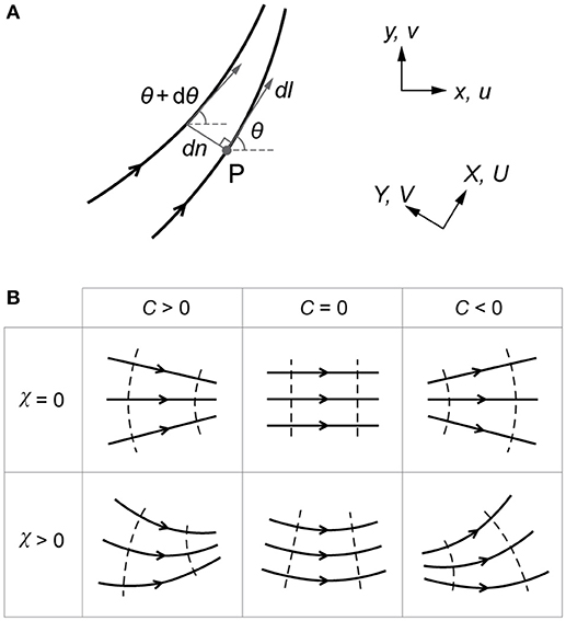
Figure 1. (A) Symbols defining flowline geometry. (B) Convergence C and curvature χ for archetypal flow patterns. Adapted from Ng (2015).

The directions n and l are known from θ or θ. Using vector calculus, we find that the definitions in Equation (3) can be written as

$\begin{array}{l}C=-(k\times \theta ).\nabla \theta =-\left(-s\frac{\partial \theta }{\partial x}+c\frac{\partial \theta }{\partial y}\right)\\ =-\left(\frac{\partial c}{\partial x}+\frac{\partial s}{\partial y}\right)=-\nabla .\theta & (4)\end{array}$

and

$\begin{array}{l}\chi =\theta .\nabla \theta =\left(c\frac{\partial \theta }{\partial x}+s\frac{\partial \theta }{\partial y}\right)\\ =\left(\frac{\partial s}{\partial x}-\frac{\partial c}{\partial y}\right)=k.(\nabla \times \theta ),& (5)\end{array}$

where k is the unit vector in the vertical. These results, given here for the first time in the glaciological context, show that −C (what we call “flow divergence” in this paper) is the divergence of the flow-direction vector field θ, and χ is the magnitude of the curl of θ. Despite similarities, C and χ are not the ice flux divergence ∇.q and vorticity ω = k.(∇×u) = (∂v/∂x – ∂u/∂y)/2, which involve flow speed. Moreover, while χ measures the local curvature of flowlines, C measures the local curvature of the curves orthogonal to flowlines and is positive when these curves are concave toward flow (dashed, Figure 1B). This orthogonality motivates a generalized vector curvature field (χ –C)^T, as expressed in Equation (A4) in the Appendix. Equations (4) and (5) did not feature in Ng's (2015) study. These crucial results enable our subsequent analysis in the sections ‘Areal Integrals and Symmetry Breaking', ‘Flowlines and Balance Flux' and ‘Ice-Flow Tributarization and the Tower Plot.'

Ice must deform in any converging/diverging or curving flow, so C and χ must be linked to strain rates. By considering how fast ice shortens laterally as it moves through any position, Ng (2015) deduced that locally C equals the lateral compressive strain rate divided by the flow speed U. Analogously, it turns out that curvature χ is the transverse shear strain rate divided by U. Specifically we have

$\begin{array}{rc}C=-\frac{1}{U}\frac{\partial V}{\partial Y}\text{\hspace{1em}and\hspace{1em}}\chi =\frac{1}{U}\frac{\partial V}{\partial X},& (6)\end{array}$

where V is the lateral component of velocity when the local coordinate system about each position P is rotated to (X Y)^T, with X pointing along flow (Figure 1A). For completeness, we give a formal derivation of both of these relationships in the Appendix.

Why consider C and χ instead of strain rates, if they differ merely by a speed normalization? One reason is that C and χ reflect strain rates resolved in two special directions associated with the ice flow locally; the spatial fields of those resolved components are rarely examined. A second reason, linked closely to our (geo)morphological interests in this paper, is that C and χ quantify the geometric pattern of flowline systems directly, whereas strain rates do not—it is not possible to conceive how fast flowlines constrict or splay by inspecting strain rates alone.

Areal Integrals and Symmetry Breaking

A study of the areal integrals of C and χ produces the first insights on ice-flow organization. Over a given area, the average value of C reflects whether flowlines within it converge or diverge overall, and the average value of χ whether they curve leftward or rightward overall. By using the signs of $\overline{C}$ and $\overline{\chi }$ to classify sub-domains, we can begin to deconstruct complex flow patterns across glaciers and ice sheets.

Applying Gauss's Theorem to Equation (4) and Stokes's Theorem to Equation (5) to an area S bounded by the curve Γ yields

$\begin{array}{cc}S\overline{C}={\displaystyle \underset{S}{\iint }C}\text{\hspace{0.17em}d}A=-{\displaystyle \underset{S}{\iint }\nabla .\theta \text{\hspace{0.17em}d}A}=-{\displaystyle \underset{\Gamma }{\oint }\theta ·\widehat{n}\text{\hspace{0.17em}d}r}& (7)\end{array}$

and

$\begin{array}{cc}S\overline{\chi }={\displaystyle \underset{S}{\iint }\chi \text{d}A}={\displaystyle \underset{S}{\iint }(\nabla \times \theta ).\text{d}A}={\displaystyle \underset{\Gamma }{\oint }\theta .\text{d}r},& (8)\end{array}$

which show that the signs of the convergence and curvature integrals—thus, sgn($\overline{C}$) and sgn($\overline{\chi }$) also—are governed by the sign of the (boundary) line integral of flow-direction normals and flow-direction parallels, respectively. Only the angle between θ and the enclosing boundary matters, as flow speed is excluded. Equations (7) and (8) are conservative in the sense that different distributions of C and χ (i.e., different flowline patterns) in the area can have the same total integrals.

Figure 2A shows an example where the convergence integral and $\overline{C}$ are both positive because θ points into S along much of the boundary and out from S along a short stretch. No contribution to $\overline{C}$ comes from those stretches following flowlines (dashed). Flow in the area must converge overall, regardless of the convergence variations and the actual pattern of flowlines within it. An opposite case can be conceived by reversing the flow directions.

FIGURE 2

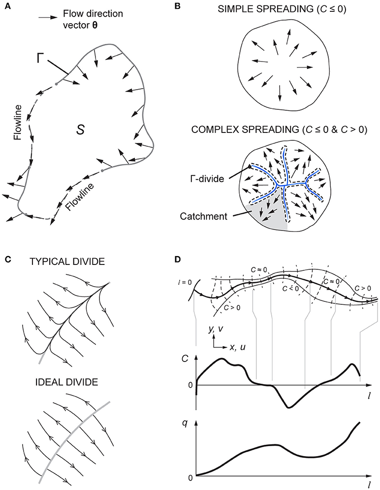
Figure 2. Anatomy of the flow-direction field and flowline system. (A) Test area for the convergence integral in Equation (7). (B) Symmetry-breaking transition from simple to complex ice-sheet flow. (C) Flowline configurations in the neighborhood of ice divides. (D) Accumulation of ice-flux density q on a flowline controlled by varying convergence and divergence along its course.

This framework sheds light on the “symmetry breaking” of flow on spreading ice sheets and ice caps (Figure 2B). By this we mean the transition from simple spreading that is divergent everywhere even if not perfectly radial, as often seen on small ice caps, to complex spreading in large ice sheets where ice flow occurs in distinct basins/catchments, in which it often converges (e.g., in tributary ice-stream systems; Ng and Conway, 2004; Ng, 2015). Symmetry breaking specifically involves the bifurcation from C ≤ 0 only to C ≤ 0 and C > 0 (Figure 2B), not just the azimuthal component of θ becoming non-zero. As noted in the Introduction, Nye's (1991, 1993) analysis concerns the local configuration of strain rates near spreading centers (e.g., summits) and not this behavior, nor the global pattern of flow across an ice mass.

The existence of ice divides between drainage basins turns out to be critical to symmetry breaking. On most divides, ice flow occurs in roughly or nearly opposite directions on the two sides. A small velocity along the divide allows θ to vary continuously—even if rapidly—across it, so C at the divide is finite and negative (Figure 2C, upper); this can be shown by applying Equation (7) to a strip of area containing a divide segment, and taking the mathematical limit as its width goes to zero. In the ideal case where the component of velocity along the divide is identically zero, θ is opposite on the two sides and switches discontinuously across the divide, and so is undefined at the divide (Figure 2C, lower); in this case, the mathematical limit implies C = –∞ there. Consequently, any small area containing a divide (or a spreading center) has $\overline{C}$ < 0, implying that divide networks are sources of flow divergence.

For an ice sheet with N catchments, we can partition its total convergence integral as

$\begin{array}{rcl}{(S\bar{C})}_{\text{Icesheet}}& =& {\displaystyle \underset{\text{Divides}}{\iint }}C\text{ d}A+{\displaystyle \sum _{i=1}^N}{\displaystyle \underset{\text{Catchment}i}{\iint }}C\text{ d}A\end{array}$

$\begin{array}{rcl}=& {\displaystyle \underset{\Gamma -\text{Divides}}{\oint }}-\theta ·\widehat{\text{n}}\text{d}r+{\displaystyle \sum _{i=1}^N}{\displaystyle \underset{\text{Catchment}i}{\iint }}C\text{d}A,& (9)\end{array}$

where “Γ-divide” is drawn tightly around divide networks (Figure 2B), including any isolated ones on ice domes and rises. Overall spreading of the ice sheet implies that the left-hand side of Equation (9) is always negative [as can be shown with Equation (7)], but a stronger negative contribution from divides [first term on the right-hand side of Equation (9)] will render the Σ-term positive, such that contributions from some or all catchments must be positive. This result means that convergent ice flow will always occur in some catchments (even though ${\overline{C}}_{\text{Icesheet}}$ < 0) when a sufficiently strong divide network forms in the ice-sheet interior (e.g., Figure 2B). Another important deduction from Equation (9) is that the bifurcation yielding C > 0 in some areas always requires C < ${\overline{C}}_{\text{Icesheet}}$ (< 0) to emerge elsewhere.

In this analysis, we are not merely restating the common glaciological appreciation that ice sheet flow is characterized by catchments and divides; in fact, this configuration is so familiar that it may not come across as something to be studied or quantifiable. Our analysis explicitly predicts the conservation of spatial rates of flowline merging/splitting across this system. We also emphasize that our topological arguments above do not explain the ice-flow thermomechanics creating divides and catchments in the first place; however, they do illustrate why the U versus C distribution for the Antarctic Ice Sheet (Figure 3A; Ng, 2015) spans both signs in C. We return to examine this distribution's shape after investigating how C affects the ice flux along flowlines (next section ‘Flowlines and Balance Flux').

FIGURE 3

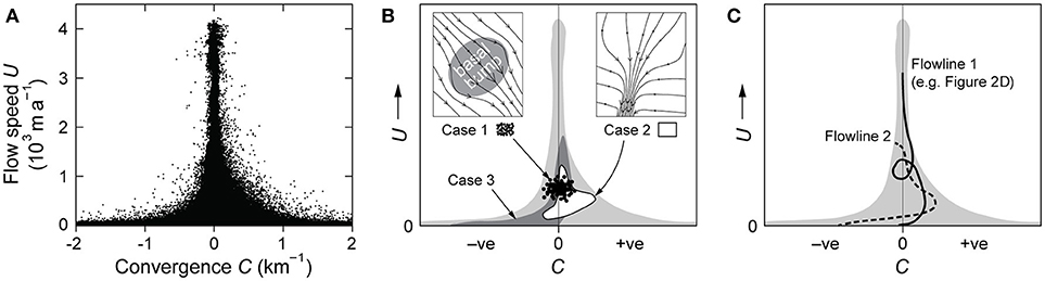
Figure 3. Different ways of decomposing the tower distribution. (A) Plot of U versus C for the Antarctic Ice Sheet; data from Ng (2015). (B) Hypothetical U–C data associated with different ice-flow structures, overlaid on the tower distribution from panel (A); cases 1 to 3 are explained in the text. (C) Hypothetical trajectories of U and C along two flowlines.

This analysis informs other aspects of ice flow at catchment scale, some having analogues in mountain and hillslope geomorphology. Divides (loci of C < 0) with large negative C may be described as sharp, divides with less negative C as blunt (Figure 2C); the latter portray rounded ridges of divergence, and C can vary in intensity across a divide network (Figure 2B). Divides and ridges may also form inside a catchment, in which case flow convergence elsewhere in the catchment must be increased in view of the conservative property of its areal convergence integral. On a parallel flow, perturbation of flow directions to create convergence must produce divergence in neighboring areas. The spatial alternation of divergent and convergent flow during tributary formation in ice-stream systems (Ng, 2015; e.g., Figure 4C) can be understood in terms of such bifurcation of C.

FIGURE 4

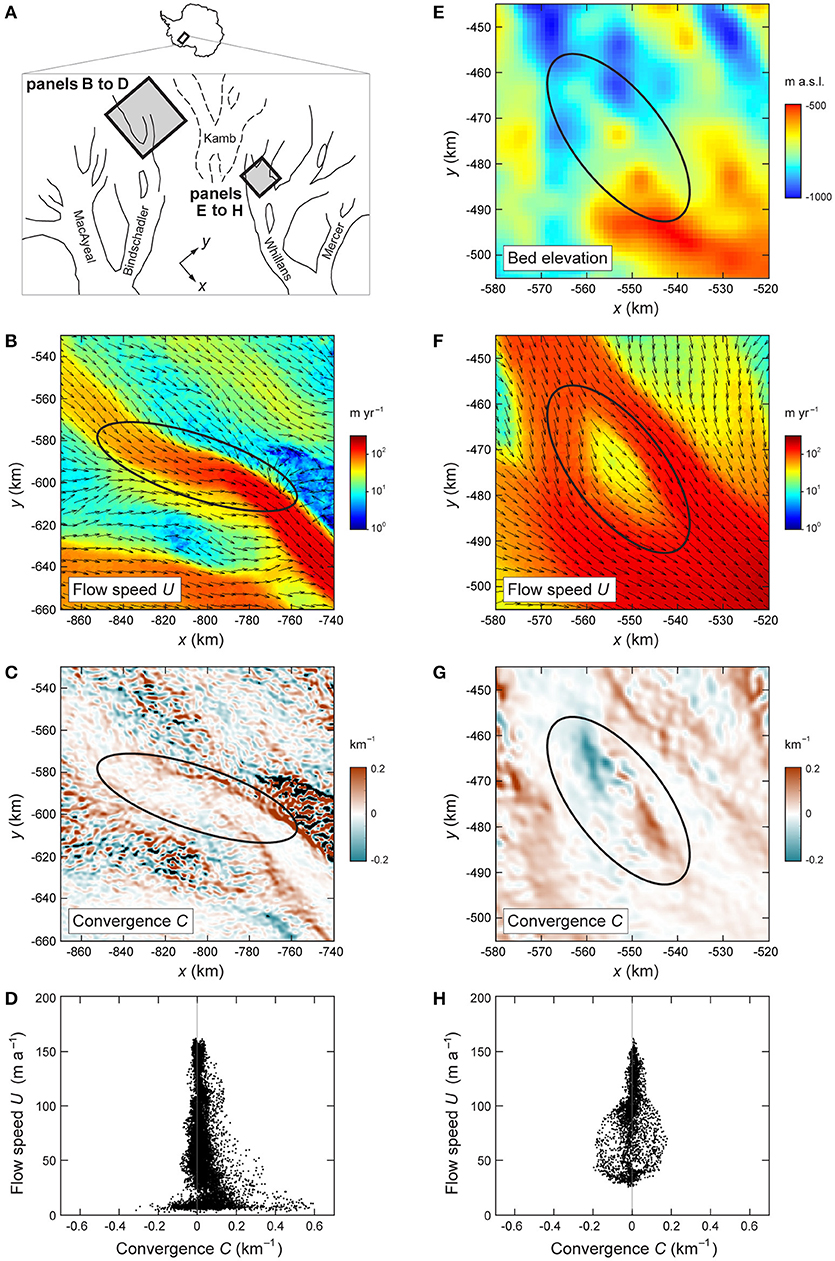
Figure 4. Two types of flow structures on ice streams and their speed–convergence (U–C) signatures. (A) Map of ice streams along West Antarctica's Siple Coast, locating the areas studied in the later panels. Panels (B–D) pertain to a fast-flow onset zone on Bindschadler Ice Stream. Panels (E–H) pertain to an upstream region of Whillans Ice Stream. (B,F) Surface flow speed U and flow-direction unit vectors derived from the dataset of Rignot et al. (2011). (E) Bed elevation from Bedmap2 (Fretwell et al., 2013). (C,G) Flow convergence C from Ng's (2015) dataset. (D,H) Plots of U against C for the areas enclosed by ellipses in (B–C) and (E–G), respectively. Both plots are located well within and near the base of the tower distribution in Figure 3A.

Flowlines and Balance Flux

Next we explore the relevance of flow convergence and divergence for the ice flux routed along flowlines. This yields an understanding of how their geometry influences the pattern of ice speeds and fluxes across an ice mass. Let H(x, y, t) denote the ice mass's thickness, a(x, y, t) its net mass balance, and t time. Define ice flux density vectorially as q = qθ, with q = q(x, y, t) ≥ 0 as its magnitude. The ice-flow direction is assumed to be depth-invariant. Writing q in terms of θ, rather than as H times the column-averaged ice velocity $\overline{\mathbf{\text{u}}}$ (which is the usual practice), facilitates an analysis based directly on flowline configuration. Now, conservation of mass implies

$\begin{array}{cc}\frac{\partial H}{\partial t}+\nabla .q\equiv \frac{\partial H}{\partial t}+\theta .\nabla q+q(\nabla .\theta )=a.& (10)\end{array}$

By substituting C = −∇.θ from Equation (4) and defining the curvilinear coordinate l to follow a flowline such that

$\begin{array}{rc}\frac{\partial x}{\partial l}=c\text{\hspace{1em}and\hspace{1em}}\frac{\partial y}{\partial l}=s,& (11)\end{array}$

Equation (10) can be converted to

$\begin{array}{rc}\frac{\partial H}{\partial t}+\frac{\partial q}{\partial l}=a+Cq.& (12)\end{array}$

As the flowline's curvature is χ = ∂θ/∂l (Equation (3)), ice flow direction varies along it according to

$\begin{array}{rc}\theta (l,t)={\displaystyle {\int }_0^l}\chi \text{d}l+\theta (l=0,t),& (13)\end{array}$

in which l = 0 locates its starting point on the divide.

Equation (12) describes mass conservation instantaneously along any flowline (whether its trajectory migrates over time) and can be used on multiple flowlines to track the evolution of H and the ice surface in three dimensions. Since a flowline has zero width, this description differs from the mass conservation equation in 2.5-dimensional “flowtube” glaciological models (p. 275, Van der Veen, 2013; Passalacqua et al., 2016), which addresses flow of a finite width between two flowlines.

By assuming orthogonality between flowlines and elevation contours of the ice surface, Reeh (1988) derived a result like Equation (12) with its last term Cq replaced by q/R, where R is the radius of curvature of the contours where they meet a flowline. Such orthogonality is valid where the shallow ice approximation applies, but may break down where lateral/longitudinal stress gradients in the ice dominate, e.g., at ice-stream shear margins. But whether orthogonality holds, Equation (12) establishes a precise connection between the flux field q and flow differential geometry—by virtue of C = −∇.θ.

This connection is especially clear when we consider the balance fluxes and velocities (Budd and Warner, 1996) which keep the ice surface topography constant. Under steady state (∂/∂t ≡ 0) Equation (12) becomes

$\begin{array}{rc}\frac{\text{d}{q}_0}{\text{d}l}=a(l)+C(l)q_0,& (14)\end{array}$

which shows that the balance flux q₀ increases along the flowline as a result of mass balance and lateral gain from (/loss to) flow convergence (/flow divergence). The final term here, describing lateral focussing of ice flux onto the flowline when C > 0 and dilation of the flux when C < 0, feeds back positively and negatively (respectively) on the rate of change of q₀ (Figure 2D). In contrast, the curvature χ has no bearing on the flux accumulation. On a flowline with known ice thickness profile H(l), the balance velocity is given by

$\begin{array}{rc}{\overline{\text{u}}}_0={\mathit{\text{U}}}_0\theta ,\text{ where }{\mathit{\text{U}}}_0={\mathit{\text{q}}}_0/\mathit{\text{H}}.& (15)\end{array}$

Balance flux/velocity fields are useful for visualizing the flow pattern across an ice mass, supplying gridded-velocity estimates for glaciological studies, detecting unsteady flow regions (those exhibiting dynamical and/or elevation changes) through comparison with satellite-/field-measured surface velocities, and defining states for initializing numerical ice-flow simulations (Budd and Warner, 1996; Bamber et al., 2000a,b; Fricker et al., 2000; Wu and Jezek, 2004; LeBrocq et al., 2006; Williams et al., 2014). A common approach of computing balance flux fields is to solve the steady version of Equation (10) for q = (q_x q_y)^T on a rectangular grid under prescribed mass balance, with the Cartesian flux components satisfying q_y/q_x = tanθ, for consistency with flow directions (e.g., Budd and Warner, 1996; Fricker et al., 2000; Wu and Jezek, 2004; LeBrocq et al., 2006). Typically the θ-field is derived from the known surface topography by assuming that flow occurs in the direction of steepest surface slope, which is equivalent to Reeh's (1988) assumption above. Variations in numerical scheme exist, as the misalignment in orientation between the coordinate axes and flow directions yields different approximations for the flux routing between adjacent grid points or cells. Another approach of computing balance flux uses the flowtube idea by summing mass balance between neighboring flowlines from the divide to various positions downstream (Joughin et al., 1997; Testut et al., 2003), and its accuracy depends on the flowline separation. Recently, Brinkerhoff and Johnson (2015) put forward a numerical algorithm based on the finite-element approach that uses a spatially-unstructured grid to reduce the errors on flux routing and thus improve upon these methods.

Equation (14) unravels the topological basis of balance flux fields by showing that q₀(x, y) obeys a continuum set of initial-value problems along flowlines. Thus it motivates a new way of calculating the fields, in which these flowline problems are solved, given input data for the convergence field C(x, y), mass balance a(x, y), and flowline trajectories determined from the curvature field χ(x, y) via Equation (13). Conceptually, this method amounts to a transformation or mapping of one pattern (that of flow directions) into another pattern (of ice-flux magnitude). The grid-based and flowtube approaches described above do not recognize this curvilinear mapping nor flowline differential geometry. The new method has two distinct steps: (1) The estimation of flowline trajectories (starting from divides) and estimation of C and χ along flowlines from flow directions. Both of these necessitate spatial interpolation of flow-direction data in practice, e.g., by kriging (Ng, 2015). (2) The solution of Equation (14) on each flowline for its flux profile (Figure 2D). This can be done with an Euler-based numerical scheme or analytically with an integrating factor. With q₀(l = 0) = 0 at the divide, the latter method gives

$\begin{array}{rc}{q}_0(l)=e^{-f(l)}{\displaystyle {\int }_0^l}{e}^{f(l)}a(l)\text{d}l& (16)\end{array}$

where

$\begin{array}{rc}f(l)=-\int C(l)\text{d}l.& (17)\end{array}$

The balance velocity field can then be found via Equation (15).

These insights illuminate a remarkable property of balance velocity fields of the Antarctic and Greenland Ice Sheets, which is that they predict networks of fast ice flow in roughly the same places where ice stream tributaries/trunks are indeed observed (e.g., Figure 1 of Budd and Warner, 1996; Figure 2 of Bamber et al., 2000b; Figure 5 of Wu and Jezek, 2004). Although past studies correctly attributed this prediction—in descriptive terms—to ice converging toward topographic lows or valleys in the ice surface, our theory quantifies the mechanism precisely. Equation (14) shows that the critical control in this fast-flow localization is C = −∇.θ and the mechanism involves positive feedback: the higher is q at a given position, the faster q increases along flow when C > 0 there (for a fixed local pattern of merging flowlines); in turn, the increased ice flux strengthens the feedback further downstream. Equation (14) also explains why in the grid-based and flowtube approaches, details of the calculated balance flux/velocity fields in such fast-flowing areas are critically sensitive to the grid spacing and the degree of pre-smoothing of the ice surface used to derive flow directions (Budd and Warner, 1996; Fricker et al., 2000; Testut et al., 2003; Wu and Jezek, 2004; LeBrocq et al., 2006). This is because these approaches compute the accumulation of ice flux from flow directions and gradients of flow directions (analogues of C and χ) evaluated at coordinate points some distance away from individual flowlines. Not only does the corresponding numerical discretization introduce errors to the flux accumulation when the grid is not sufficiently fine, the errors also self-amplify wherever the positive feedback operates. This problem is additional to the potential misalignment of flow directions from the directions of steepest surface slope due to stress-gradient coupling (Williams et al., 2014) or a slippery bed (Gudmundsson, 2003). In contrast, the method of Equation (14) can more robustly capture the fast-flow features because it calculates balance flux along the curvilinear trajectories of the flowlines themselves, before the results are interpolated back onto a regular grid.

The same theory allows us to deduce balance flux/velocity variations across ice-divide networks. As each limb of the divide is a flowline with C < 0 (see the section ‘Areal Integrals and Symmetry Breaking'), Equation (14) shows that negative feedback keeps q₀ small in the corresponding flux accumulation, despite input from snowfall (a > 0).

Ice-Flow Tributarization and the Tower Plot

How does the differential-geometry framework help us understand ice-stream spatiodynamics? We consider this topic by using insights from the previous sections.

In ice-stream networks, fast (streaming) flow occurs in ice-stream trunks and interconnecting tributaries that branch and braid around slow-flowing ice domes and rises; some tributaries penetrate far into the interior to draw ice (e.g., Joughin et al., 1999; Rignot et al., 2011; Ng, 2015). This “tributarization” behavior, which involves non-uniform convergent and divergent flow in individual catchments and is exemplified by the ice streams along the Siple Coast in West Antarctica (i.e., the ice streams named Mercer, Whillans, Kamb, Bindschadler, and MacAyeal in Figure 4A), has been theorized to originate from a spatial instability due to nonlinear coupling between ice-flow thermomechanics, basal sliding and subglacial hydrology (Fowler and Johnson, 1996). Numerical simulations of the instability have been used to predict the spacing and branching of tributaries (Payne and Dongelmans, 1997; Sayag and Tziperman, 2011; Kyrke-Smith et al., 2015), in idealized model configurations less complex (irregular and highly branched) than the observed networks. While future numerical simulations will no doubt strive for more realism and better physics, a separate and complementary approach of probing the tributarization dynamics—in both real and model systems—is to study their statistical imprint on a plot of U versus C (or U versus χ). As Ng (2015) reported, the tower-shaped U–C plot for Antarctica (Figure 3A) implies that fast flow cannot converge or diverge as much as slow flow, and this property is found for individual catchments as well. The bulk tower distribution is not exactly symmetrical—excess convergence in 20 ≲ U ≲ 200 m a⁻¹ yields $\overline{C}$ ≈ +0.012 km⁻¹ for these mid-range speeds.

Our theory provides a roadmap for analyzing these properties and the tower's composition. We know from the section ‘Areal Integrals and Symmetry Breaking' that the tower's span reflects ice-flow symmetry breaking causing C to bifurcate into both signs. But symmetry breaking can involve different ice-flow structures on a variety of length scales across the ice sheet. Each structure has its own spatial fields of C and U, and we can inquire its “signature”—ask how these data plot against each other—on the U–C plot. For instance, over distances on the order of ~10 km, bifurcation in sgn(C) may arise from ice flow over and around a basal bump or sticky/slippery spot (Gudmundsson, 2003; Ely et al., 2017). Assuming an otherwise parallel flow, we expect the speed differential and flow-direction changes induced by such basal perturbation to yield a data cloud on the U–C plot that straddles C > 0 and C < 0 and falls in a specific speed range; the degree of scatter of this cloud presumably increases with the perturbation amplitude. The hypothesized signature of such structure on the tower plot is shown in Figure 3B (Case 1). A real example of a data cloud from ice flow over a basal topographic bump (probably also a sticky spot) from Whillans Ice Stream is detailed in Figures 4E–H. In this example, divergent flow upstream of the bump and convergent flow downstream creates a “dipole” in C (Figure 4G), whose values plot roughly symmetrically about C = 0 in Figure 4H. A similar dipole would occur in the spatial field of the compressive component of the strain-rate tensor resolved in the direction locally perpendicular to the ice-flow direction, but, as explained in the section ‘Flow Convergence and Curvature', C directly quantifies the geometrical pattern of the flowlines, whereas strain rates do not.

In contrast, the onset zone of an ice stream may have an asymmetric signature on the U–C plot, due to the combination of convergent flow at its lateral shear margins, less convergent but faster flow in the stream, and divergent slow flow outside the margins (e.g., Case 2 in Figure 3B). Figures 4B–D detail a real example of such signature compiled from data from the onset area of a tributary of Bindschadler Ice Stream. The signature is expected to be still different if we go upscale to consider a whole catchment with convergent flow inside it (assuming short-scale structures are absent) and divergent flow on the divide boundary (e.g., Case 3 in Figure 3B; the section ‘Areal Integrals and Symmetry Breaking'). A real example is not illustrated for this case as we currently lack reliable convergence estimates for the slow-flowing interior of Antarctica (Ng, 2015). These examples suggest that a systematic geomorphological classification of different ice-flow structures can help us understand how their signatures together make up the tower distribution. We proffer this idea for future research to tackle.

Another way of understanding the tower distribution, based on the balance-flux theory (the section ‘Flowlines and Balance Flux'), decomposes it as the sum of U and C data from individual flowlines, which trace distinct trajectories on the plot (Figure 3C) according to the flux accumulation described by Equations (14) to (17). Variations in ice thickness along each flowline will determine how ice flux converts to speed, and the flux accumulation implies a spatially non-local relationship between U and C. But we expect most flowlines entering ice-stream networks to trace ascending trajectories in the plot (Figure 3C), given the general trends of flux increase along flow and ice-thickness reduction toward the ice-sheet margin—aided in some cases by the retrograde bed slope of ice-stream trunks and tributaries. Although real ice sheets are not at steady state, deviations from this should modify the bulk distribution only slightly.

A specific control behind the shape of the tower distribution for Antarctica may also be identified. Ng (2015) interpreted the tower's flanks, which follow U ∝ |C|^−1.4 approximately, as suggesting a constant upper limit to lateral strain rates, U|C| [see Equation (6)]. Given the rheological link of strain rates to stresses, we think that such limit reflects an intrinsic ceiling to the glaciological driving stresses in the ice sheet; e.g., 4-km thick ice with surface slopes of ~10⁻³ cannot produce driving stresses far above ~0.4 bar in order-of-magnitude terms. Equation (6) shows U|χ| as a strain-rate magnitude, and so, for the same reason, we expect a U–χ plot to exhibit a tower shape also.

In this connection, the large-scale symmetry breaking responsible for catchment–divide formation (Case 3, Figure 3B) anticipates a U-C distribution with excess convergence at the mid-range speeds and excess divergence at the low speeds of divides. Although the tower in Figure 3A does not lean visibly in this way, its asymmetry is consistent with this prediction. The divergence signal of divides may be obscured because estimates of C at low speeds U ≲ 20 m a⁻¹ are strongly corrupted by errors/noise in the satellite-measured flow directions, as is evident from the “chaotic” convergence pattern in slow-flow areas (Ng, 2015). Our interpretation here finds further support because the U–C plot compiled from balance velocities is lopsided with a strong divergence bias at low U [Supplementary Figure 6B of Ng (2015)]. Future calculation of Antarctica's convergence map should use more accurate velocity data to resolve the slow part of the U-C plot.

A final note concerns the ability of balance-velocity models to mimic ice-stream networks. If, as posited in many of these models, ice-flow directions are largely determined by ice surface slope, then the spatial pattern of slopes, ridges and valleys across the ice sheet must precondition the tower distribution. Specifically, the tower shape means that slope aspects are arranged such that their spatial variation is less in faster-flowing areas. Whatever the cause of this, we infer that evolution of the surface topography is integral to ice-stream tributarization. But a proper examination of how the ice-dynamical instability controls the U-C distribution is beyond the scope of this paper.

Conclusions

Herein, our study of the flow-direction field θ has yielded a new rigorous language for addressing ice-flow topology. By using the new-found relationships in Equations (4) and (5), we made precise connections between the differential geometry of θ and perceptible aspects of flowline patterns, and explored their implications for ice-flux routing and the symmetry breaking inherent in ice-stream networks. The spatial complexity of flow is ultimately the outcome of nonlinear rheology, thermomechanical processes and boundary conditions, but insights into its origin can be gained by inspecting flow directions. While the continuum description of ice flow is well established, ideas of how this complexity arises and productive ways of describing and analyzing it are barely in their infancy. With the recent explosion of observational velocity datasets, we think that combining numerical simulations and the kind of analytical work undertaken here is a promising way to advance our understanding of pattern formation in ice flow. An interesting avenue is to cast the continuum model in curvilinear terms using convergence C and curvature χ [going beyond mass conservation in Equation (12)] to explain the time-dependent dynamics of these fields and formulate pattern-based theories of ice-streaming instability.

Author Contributions

FN developed the theory and wrote the manuscript. GG and EK contributed editing suggestions and advice on how to illustrate the theory.

Conflict of Interest Statement

The authors declare that the research was conducted in the absence of any commercial or financial relationships that could be construed as a potential conflict of interest.

Acknowledgments

FN acknowledges the support of a Leverhulme Trust Research Fellowship in 2017-18 (no. RF-2017-320), which funded this study. We thank two reviewers and the editor for their helpful comments on our manuscript.

References

Bamber, J. L., Hardy, R. J., and Joughin, I. (2000a). An analysis of balance velocities over the Greenland ice sheet and comparison with synthetic aperture radar interferometry. J. Glaciol. 46, 67–74. doi: 10.3189/172756500781833412

CrossRef Full Text | Google Scholar

Bamber, J. L., Vaughan, D. G., and Joughin, I. (2000b). Widespread complex flow in the interior of the Antarctic Ice Sheet. Science 287, 1248–1250. doi: 10.1126/science.287.5456.1248

PubMed Abstract | CrossRef Full Text | Google Scholar

Brinkerhoff, D., and Johnson, J. (2015). A stabilized finite element method for calculating balance velocities in ice sheets. Geosci. Model Dev. 8, 1275–1283. doi: 10.5194/gmd-8-1275-2015

CrossRef Full Text | Google Scholar

Budd, W. F., and Warner, R. C. (1996). A computer scheme for rapid calculations of balance-flux distributions. Ann. Glaciol. 23, 21–27. doi: 10.3189/S0260305500013215

CrossRef Full Text | Google Scholar

Clark, C. D. (1997). Reconstructing the evolutionary dynamics of former ice sheets using multi-temporal evidence, remote sensing and GIS. Quat. Sci. Rev. 16, 1067–1092. doi: 10.1016/S0277-3791(97)00037-1

CrossRef Full Text | Google Scholar

Ely, J. C., Clark, C. D., Ng, F. S. L., and Spagnolo, M. (2017). Insights on the formation of longitudinal surface structures on ice sheets from analysis of their spacing, spatial distribution, and relationship to ice thickness and flow. J. Geophys. Res. Earth Surf. 122, 961–972. doi: 10.1002/2016JF004071

CrossRef Full Text | Google Scholar

Fahnestock, M., Scambos, T., Moon, T., Gardner, A., Haran, T., and Klinger, M. (2016). Rapid large-area mapping of ice flow using Landsat 8. Remote Sens. Environ. 185, 84–94. doi: 10.1016/j.rse.2015.11.023

CrossRef Full Text | Google Scholar

Fowler, A. C., and Johnson, C. (1996). Ice-sheet surging and ice-stream formation. Ann. Glaciol. 23, 68–73. doi: 10.3189/S0260305500013276

CrossRef Full Text | Google Scholar

Fretwell, P., Pritchard, H. D., Vaughan, D. G., Bamber, J. L., Barrand, N. E., Bell, R., et al. (2013). Bedmap2: improved ice bed, surface and thickness datasets for Antarctica. Cryosphere 7, 375–393. doi: 10.5194/tc-7-375-2013

CrossRef Full Text | Google Scholar

Fricker, H. A., Warner, R. C., and Allison, I. (2000). Mass balance of the Lambert Glacier–Amery Ice Shelf system, East Antarctica: a comparison of computed balance fluxes and measured fluxes. J. Glaciol. 46, 561–570. doi: 10.3189/172756500781832765

CrossRef Full Text | Google Scholar

Gudmundsson, G. H. (2003). Transmission of basal variability to a glacier surface. J. Geophys. Res. Earth Surf. 108:2253. doi: 10.1029/2002JB002107

CrossRef Full Text | Google Scholar

Joughin, I., Fahnestock, M., Ekholm, S., and Kwok, R. (1997). Balance velocities of the Greenland Ice Sheet. Geophys. Res. Lett. 24, 3045–3048. doi: 10.1029/97GL53151

CrossRef Full Text | Google Scholar

Joughin, I., Gray, L., Bindschadler, R., Price, S., Morse, D., Hulbe, C., et al. (1999). Tributaries of West Antarctic ice streams revealed by RADARSAT interferometry. Science 286, 283–286. doi: 10.1126/science.286.5438.283

PubMed Abstract | CrossRef Full Text | Google Scholar

Kyrke-Smith, T. M., Katz, R. F., and Fowler, A. C. (2015). Subglacial hydrology as a control on emergence, scale, and spacing of ice streams. J. Geophys. Res. Earth Surf. 120, 1501–1514. doi: 10.1002/2015JF003505

CrossRef Full Text

LeBrocq, A. M., Payne, A. J., and Siegert, M. J. (2006). West Antarctic balance calculations: impact of flux-routing algorithm, smoothing algorithm and topography. Comput. Geosci. 32, 1780–1795. doi: 10.1016/j.cageo.2006.05.003

CrossRef Full Text | Google Scholar

Ng, F., and Conway, H. (2004). Fast-flow signature in the stagnated Kamb Ice Stream, West Antarctica. Geology 32, 481–484. doi: 10.1130/G20317.1

CrossRef Full Text | Google Scholar

Ng, F. S. L. (2015). Spatial complexity of ice flow across the Antarctic Ice Sheet. Nat. Geosci. 8, 847–850. doi: 10.1038/ngeo2532

CrossRef Full Text | Google Scholar

Nye, J. F. (1983). Monstars on glaciers. J. Glaciol. 29, 70–77. doi: 10.3189/S0022143000005153

CrossRef Full Text | Google Scholar

Nye, J. F. (1986). Isotropic points on glaciers. J. Glaciol. 32, 363–365. doi: 10.3189/S0022143000012041

CrossRef Full Text | Google Scholar

Nye, J. F. (1991). The topology of ice-sheet centres. J. Glaciol. 37, 220–227. doi: 10.3189/S0022143000007231

CrossRef Full Text | Google Scholar

Nye, J. F. (1993). A topological approach to the strain-rate pattern of ice sheets. J. Glaciol. 39, 10–14. doi: 10.3189/S0022143000015677

CrossRef Full Text | Google Scholar

Passalacqua, O., Gagliardini, O., Parrenin, F., Todd, J., Gillet-Chaulet, F., and Ritz, C. (2016). Performance and applicability of a 2.5-D ice-flow model in the vicinity of a dome. Geosci. Model Dev. 9, 2301–2313. doi: 10.5194/gmd-9-2301-2016

CrossRef Full Text | Google Scholar

Payne, A. J., and Dongelmans, P. W. (1997). Self-organization in the thermomechanical flow of ice sheets. J. Geophys. Res. Earth Surf. 102, 12219–12233. doi: 10.1029/97JB00513

CrossRef Full Text | Google Scholar

Reeh, N. (1988). A flow-line model for calculating the surface profile and the velocity, strain-rate, and stress fields in an ice sheet. J. Glaciol. 34, 46–54. doi: 10.3189/S0022143000009059

CrossRef Full Text | Google Scholar

Rignot, E., Mouginot, J., and Scheuchl, B. (2011). Ice flow of the Antarctic Ice Sheet. Science 333, 1427–1430. doi: 10.1126/science.1208336

PubMed Abstract | CrossRef Full Text | Google Scholar

Sayag, R., and Tziperman, E. (2011). Interaction and variability of ice streams under a triple-valued sliding law and non-Newtonian rheology. J. Geophys. Res. Earth Surf. 116:F01009. doi: 10.1029/2010JF001839

CrossRef Full Text | Google Scholar

Testut, L., Hurd, R., Coleman, R., Rémy, F., and Legrésy, B. (2003). Comparison between computed balance velocities and GPS measurements in the Lambert Glacier basin, East Antarctica. Ann. Glaciol. 37, 337–343. doi: 10.3189/172756403781815672

CrossRef Full Text | Google Scholar

Van der Veen, C. J. (2013). Fundamentals of Glacier Dynamics. Boca Raton, FL: CRC Press.

Google Scholar

Williams, C. R., Hindmarsh, R. C. A., and Arthern, R. J. (2014). Calculating balance velocities with a membrane stress correction. J. Glaciol. 60, 294–304. doi: 10.3189/2014JoG13J092

CrossRef Full Text | Google Scholar

Wu, X., and Jezek, K. C. (2004). Antarctic ice-sheet balance velocities from merged point and vector data. J. Glaciol. 50, 219–230. doi: 10.3189/172756504781830042

CrossRef Full Text | Google Scholar

Appendix

Consider a local rotation of the coordinate system x = (x y)^T at any point P to X = (X Y)^T = Rx, where

$\begin{array}{rc}\text{R}=\left(\begin{array}{cc}c& s\\ -s& c\end{array}\right),& (\mathrm{A1})\end{array}$

such that X points along flow (Figure 1A). In the rotated coordinates, flow velocity becomes

$\begin{array}{rc}\text{U}=\left(\begin{array}{c}U\\ V\end{array}\right)=\text{R}\text{u}=\left(\begin{array}{c}cu+sv\\ 0\end{array}\right)& (\mathrm{A2})\end{array}$

(Equation (1) implies su = cv), and the gradient of any variable f is

$\begin{array}{cc}{\nabla }_{XY}f=\left(\begin{array}{c}\partial f/\partial X\\ \partial f/\partial Y\end{array}\right)=R\nabla f.& (\mathrm{A3})\end{array}$

Thus, one can verify that in the rotated system, C and χ retain their meanings as originally defined in Equation (3); i.e.,

$\begin{array}{cc}\left(\begin{array}{c}\chi \\ -C\end{array}\right)=\left(\begin{array}{c}\partial \theta /\partial X\\ \partial \theta /\partial Y\end{array}\right)\equiv R\nabla \theta =\left(\begin{array}{cc}c& s\\ -s& c\end{array}\right)\left(\begin{array}{c}\partial \theta /\partial x\\ \partial \theta /\partial y\end{array}\right)& (\mathrm{A4})\end{array}$

agrees with Equations (4) and (5).

The rotation transforms the velocity gradient tensor

$\begin{array}{cc}\nabla u=\left(\begin{array}{cc}\partial u/\partial x& \partial v/\partial x\\ \partial u/\partial y& \partial v/\partial y\end{array}\right)& (\mathrm{A5})\end{array}$

to

$\begin{array}{cc}{\nabla }_{XY}U=\left(\begin{array}{cc}\partial U/\partial X& \partial V/\partial X\\ \partial U/\partial Y& \partial V/\partial Y\end{array}\right)=R(\nabla u)R^T.& (\mathrm{A6})\end{array}$

Evaluating the triple product on the right-hand side here gives

$\begin{array}{rc}\left(\begin{array}{cc}\partial U/\partial X& \partial V/\partial X\\ \partial U/\partial Y& \partial V/\partial Y\end{array}\right)=\left(\begin{array}{cc}c\partial U/\partial x+s\partial U/\partial y& \chi U\\ -2\omega +\chi U& -CU\end{array}\right),& (\mathrm{A7})\end{array}$

from which we see

$\begin{array}{rc}C=-\frac{1}{U}\frac{\partial V}{\partial Y}\text{\hspace{1em}and\hspace{1em}}\chi =\frac{1}{U}\frac{\partial V}{\partial X}.& (\mathrm{A8})\end{array}$

Also, in (A7), the upper-left equation gives the longitudinal strain rate or acceleration, and the lower-left equation ∂U/∂Y = −2ω + χU (in which χU ≡ ∂V/∂X) confirms that vorticity ω = (∂V/∂X − ∂U/∂Y)/2 is invariant under the rotation.