Measurement of Air-Sea Methane Fluxes in the Baltic Sea Using the Eddy Covariance Method

1. Introduction

Methane (CH₄) is an atmospheric trace gas considered to be the second-most important greenhouse gas after carbon dioxide (CO₂). The estimated warming potential per molecule of CH₄ is 28 times greater than CO₂ over a 100-years horizon, and 72 times greater over a 20-years horizon (IPCC, 2013). The global average atmospheric concentration of CH₄ has more than doubled since the pre-industrial era, reaching values of over 1,800 ppb (WDCGG, 2015). CH₄ is emitted to the atmosphere by natural and anthropogenic sources, however, the rapid increase in the atmospheric CH₄ concentrations has been attributed to anthropogenic activities. Great uncertainties on the temporal and spatial variability of the individual sources of CH₄ still exist.

The ocean is a net source of CH₄ to the atmosphere. Considering biogenic, geological and hydrate sources, the global oceanic emissions have been estimated at 14 Tg yr⁻¹ (range 5-25) value that represent about 1–3% of the total global sources of atmospheric CH₄ (Saunois et al., 2016). Out of the total oceanic contribution, the shelf areas and estuaries account for up to 75%, being the major oceanic source (Bange et al., 1994). However, these estimates are still uncertain due to the limited availability of CH₄ data in the marine environment. The constrains on temporal and spatial resolution of CH₄ measurements have been the limiting factor to account for the diversity on the production and consumption mechanisms of CH₄, hindering our understanding of the oceanic contributions at regional scales, thus, the capacity to constrain the global emission estimates.

The Baltic Sea is a semi-enclosed basin at relatively high latitudes (Meier et al., 2014), it presents great spatial and temporal variability of surface CH₄ concentrations in open sea and in shallow coastal regions. Seasonal variations of water temperature, wind speed, and availability of organic matter have been identified to regulate CH₄ emissions to the atmosphere (Bange, 2006; Bange et al., 2010; Gülzow et al., 2013). A detailed description of the CH₄ budget at a basin scale in the Baltic Sea is still missing, and the lack of constrained air–sea exchange values is one of the major uncertainties.

Air–sea CH₄ fluxes (FCH₄) derived from bulk parameterizations and large-scale models based on surface water measurements have led to great uncertainties in the estimates of CH₄ global oceanic emissions (e.g., Bange et al., 1994; Rhee et al., 2009). Micrometeorological techniques, in contrast, allow direct estimations of turbulent fluxes at a high temporal resolution. The use of these techniques can significantly contribute to long-term monitoring of CH₄ emissions in marine environments to constrain the regional and global estimates. The improvement in the temporal resolution offered by the micrometeorological techniques can be specially important in coastal systems, where rapid terrestrial inputs due to hydrological events, upwelling events, and changes in the biogeochemical properties induce a high temporal variability of the forcing processes modulating FCH₄.

Micrometeorological techniques, such as eddy covariance (EC), have been widely used for estimation of momentum, energy, and mass fluxes in terrestrial (Baldocchi et al., 2001, and references therein), coastal (Crawford et al., 1993; Rutgersson and Smedman, 2010; Gutiérrez-Loza et al., 2018), and oceanic environments (McGillis et al., 2001; Miller et al., 2010). In marine applications, the EC method is commonly used for CO₂ and water vapor flux calculations. However, significantly less attention has been paid on FCH₄ with only a few studies existing about CH₄ measurements from EC (Yang et al., 2016a,b, 2019). Other micrometeorological techniques have been used—even to a lesser extent—for FCH₄ calculations. De Wilde and Duyzer (1995) reported the first FCH₄ estimates from micrometeorological measurements in the marine environment using the gradient method (Fowler and Duyzer, 1989). To our knowledge there are no available records of long-term FCH₄ from eddy covariance measurements or other micrometeorological techniques in the Baltic Sea.

In this study, we used 1 year of EC measurements of CH₄ at Östergarnholm site in the Baltic Sea with the following aims: (1) investigate the viability and quality of EC measurements when studying air–sea FCH₄ from a land-based station in a marine environment, (2) estimate the annual FCH₄ and the seasonal variations in the region, and (3) explore the controlling mechanisms on air–sea CH₄ exchange.

2. Methodology

2.1. Site Description

The Östergarnsholm station (57°27′N, 18°59′E) is located on a small and flat island 4 km off the eastern coast of Gotland in the Baltic Sea (Figure 1). The station has a 30-m land-based meteorological tower located on the southern tip of the island where the ground rises only 1–2 m above the sea surface. The station has being running semi-continuously since 1995 with the aim of monitoring and studying the marine atmospheric boundary layer and to assess the air-sea interaction processes (e.g., Smedman et al., 1999; Högström et al., 2008; Rutgersson et al., 2008; Sahlée et al., 2008; Rutgersson and Smedman, 2010). The station is part of the Integrated Carbon Observation System (ICOS) infrastructure.

FIGURE 1

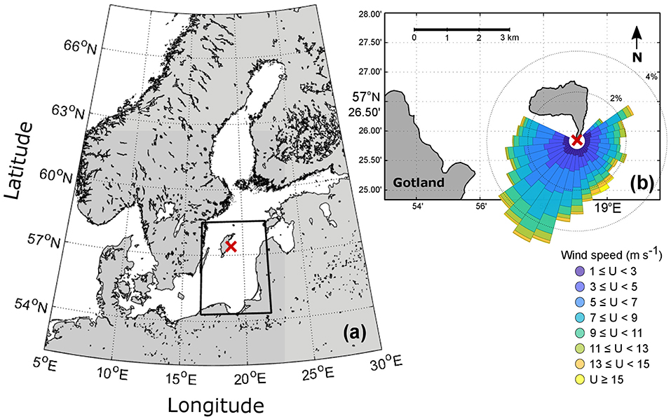
Figure 1. (a) Map of the Baltic Sea. The red mark in the central Baltic Sea indicates the location of the Östergarnsholm station; the Gotland Basin is the area within the black rectangle. (b) Location of Östergarnsholm island situated ca 4 km off from the Gotland island. The red mark indicates the location of the tower; the colors are the wind rose representing the distribution of wind speed and wind direction at the Östergarnsholm station.

The measurements at Östergarnsholm site represent open sea or coastal conditions depending on the wind direction (Rutgersson et al., 2008). For wind directions between 80° < WD < 220° the measurements from the tower are considered to be representative of open sea conditions as the wave field is undisturbed by the bathymetry and the atmospheric turbulence is not affected by coastal features (Högström et al., 2008; Rutgersson and Smedman, 2010). Processes characteristic of coastal environments are recognized for wind directions between 50° < WD < 80° and 220° < WD < 295° when the physical, biogeochemical, and hydrographical properties may be affected by the shore. In contrast, the northerly sector is strongly influenced by land, therefore data from 295° < WD < 50° are not representative for sea conditions and should not be used for air–sea interaction studies. Additionally, wind from 355° < WD < 5° is affected by the structure of the tower and should not be used for any analysis (Rutgersson et al., 2008). For this study, open sea and coastal conditions were included in the analysis (50° < WD < 295°) (see Figure 1b).

2.2. Instrumentation and Measurements

The tower was instrumented with high-frequency (20 Hz) sensors for EC measurements of FCH₄ at 9 m above the tower base. From September 2017 to September 2018, atmospheric CH₄ dry mole fractions were measured using a LI-7700 open-path gas analyzer (LI-COR, Inc., Lincoln, NE, USA). Simultaneously, the three wind-speed components were measured with a CSAT3 sonic anemometer (Campbell Scientific, Inc., Logan, UT, USA). The LI-7700 was factory calibrated just before the installation. According to the manufacturer, the factory calibration is carried out making a series of automated measurements with seven traceable reference gas concentrations under controlled conditions using an environmental chamber. The reference tanks are NIST (National Institute of Standards and Technology) certified standard gas mixtures with mole fractions of CH₄ ranging from 1 to 40 ppm (±1% accuracy). The calibration was conducted under temperature conditions of -25, 25, and 40°C in order to establish accurate relationships between the absorptance and the actual concentration.

The EC system (Figure 2) was oriented facing South, the sonic anemometer was placed on the tip of the boom and the gas analyzer LI-7700 was 0.8 m behind the sonic anemometer. The set-up of the instruments was such to minimize the air-flow disturbances, with the larger instrument (LI-7700) closer to the tower. A detailed description of the LI-7700, its functioning and calibration is given by McDermitt et al. (2011); see Sahlée et al. (2014) for the analysis of the instrument performance.

FIGURE 2

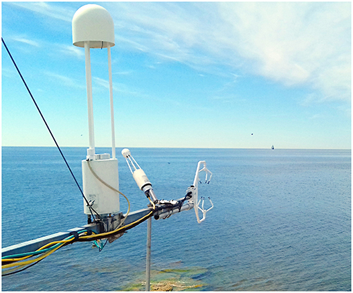
Figure 2. Photograph of the eddy covariance system set-up at level 1 (9 m) at Östergarnsholm station.

In addition to the tower measurements, water-side samplings were performed in the vicinities of the Östergarnsholm island to measure CH₄ in the seawater. Discrete samplings were carried out during the summers of 2016 and 2017. The samples were taken from a boat at three different depths (1, 10, and 18 m) using a 3 L Ruttner collector, transferred to a 60 ml gas-tight vial using a tubing and sealed with butyl rubber septa (Apodan) and aluminum caps. The samples were poisoned with 1 ml of saturated aqueous solution of mercury chloride (HgCl₂) immediately after sampling to prevent any biological activity prior to analysis. The samples were stored upside down in a dark place at 4°C until the analysis. All samples were analyzed in GEOMAR's trace gas laboratory within a few months after collection, the analysis was carried out following the static equilibration method of Bange et al. (2010). During the analysis, each individual sample was injected with 10 mL of He (99.999%), vibrated for 30 s and left to equilibrate for at least 2 h. A 9 mL subsample from the headspace was taken from each sample using a gas-tight syringe and manually injected into a gas chromatographic (GC) system (Hewlett Packard 5890 Series II) by using a 2 mL sample loop. The GC was equipped with a packed column (molsieve 5Å), He (99.999%) was used as a carrier gas with a flow rate of 30 mL min⁻¹ and a temperature of 60°C. CH₄ was detected using a flame ionization detector (FID).

A surface water CH₄ mapping campaign was performed for 2 days in late June 2018 during stable weather conditions (clear days and low winds < 3 m s⁻¹). A boat was equipped with an Ultra-portable Greenhouse Gas Analyzer (UGGA, Los Gatos Research, San Jose, CA, USA) connected to a pump-based equilibrator system. Prior to the campaign, the UGGA was calibrated using standard gases (2 ppm and 50 ppm). During boat travel (2 kn), seawater was pumped at a constant rate through a polypropylene filter and led to a silicon membrane-based equilibrator (PermSelect, Ann Arbor, USA). Seawater flows outside the silicon hollow fibers in the equilibrator, while gas penetrates the fibers toward the gas analyzer. See Paranaíba et al. (2018) for further details about the equilibrator system. The continuous water-side CH₄ concentration data was measured at 1 Hz (precision of < 2 ppb according to the manufacturer) and averaged over 15-s periods. Together with the geographic coordinates from a GPS, the data was stored on a CR1000 Campbell data logger (Campbell Scientific, Inc., Logan, UT, USA). With an estimated response time of 5 min, each data point represents a moving average integrated over ca 300 m according to the boat speed. The measurements were performed within the footprint of the tower covering all relevant wind sectors. The flux footprint area calculations—as reported by Högström et al. (2008)—indicates that for very stable conditions 60% of the fluxes are originated between 1.7 and 22 km from the tower base, and for very unstable conditions 60% of the fluxes originate between 75 and 300 m from the tower.

Water-side CH₄ values were reported in molar fraction (ppb) in order to directly compare atmospheric and oceanic measurements (see section 3.1.2 and Figure 7). Molar fractions can be further converted to concentration values—as commonly used—in nmol L⁻¹ or nmol kg⁻¹ using the solubility equation given by Wiesenburg and Guinasso (1979).

2.3. MEMENTO Database

The MarinE MethanE and NiTrous Oxide Database (MEMENTO, https://memento.geomar.de/home) collects dissolved and corresponding atmospheric CH₄ data from in situ measurements since 1986 (Table 1). We used these data to compare with the annual cycle observed from the EC results and with the water-side samples in the Baltic Sea. For this comparison, we selected data from the MEMENTO database collected within the Gotland Basin in the Baltic Sea (see Table 1). The Gotland Basin region was considered here from 54°N, 16.5°E to 58.5°N, 22°E. We defined a “coastal” sub-dataset which included the reported values from measurement sites with water depths lower than 25 m.

TABLE 1

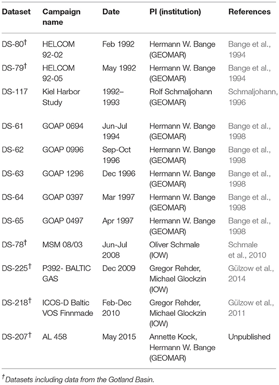
Table 1. Datasets included in the MEMENTO database with data from the Baltic Sea.

2.4. The Eddy Covariance Method

Air–sea FCH₄ were estimated using the EC method (Baldocchi et al., 1988; Aubinet et al., 2012). The general equation for the flux calculation is given by

$\begin{array}{ll}F=\overline{{\rho }_a}\overline{w^{\prime }{c}^{\prime }},& (1)\end{array}$

where ρ_a is the density of dry air, w is the vertical component of the wind speed, and c is the gas dry mole fraction. The overbar represents the temporal average and the turbulent fluctuations, indicated by the primes, are estimated from the high-frequency (20 Hz) time series of each variable through a Reynold's decomposition:

$\begin{array}{ll}x=\overline{x}+x^{\prime },& (2)\end{array}$

where x is the measured signal, $\overline{x}$ represents the time-mean value, and x′ represents the fluctuating part.

EC is a straight-forward method to determine gas fluxes. The method avoids the use of empirical constants, as the bulk methods do, it does not rely on assumptions regarding the behavior of the gas or its properties and, it does not require approximations of the atmospheric boundary layer structure (Wanninkhof et al., 2009). However, in order to fulfill the method's assumptions, a strict quality control must be applied to the data (e.g., Foken, 2008).

2.5. Data Treatment and Quality Control

We used time series of wind speed and CH₄ atmospheric dry mole fraction data obtained at the Östergarnsholm site between September 2017 and September 2018. The high-frequency raw measurements were used to calculate half-hourly values of FCH₄ using the EC method (Equation 1). Prior to the flux calculations, several selection criteria were applied to ensure high quality data representative of air–sea CH₄ exchange within the footprint.

The raw high-frequency wind components were first transformed to earth-system coordinates and the angles were corrected using a double rotation method to avoid any effects caused by the tilting of the sonic anemometer. Wind speed and wind directions were computed from the corrected wind components.

The LI-7700 gas analyzer automatically identifies CH₄ data with a -9999 flag when the sensor is not working properly. These records were removed prior to the calculations. Afterwards, a non-linear median filter algorithm was applied to the 20-Hz data over 30-min periods to eliminate outliers from the high-frequency time series (see Brock, 1986; Starkenburg et al., 2016). Half-hour periods with more than 1% (360 data points) of outliers were discarded (Foken, 2008). The turbulent fluctuations of each variable were calculated from of the de-trended time series using a Reynold's decomposition (Equation 2) over 30-min periods. A linear fit was considered for the de-trending procedure. The turbulent fluctuations were used to calculate the variance and covariance, as well as, other statistical moments used during the flux calculations and statistical analysis. Half-hour averages of each variable were then computed.

We set thresholds on some statistical parameters to ensure the homogeneity of the data and to avoid outliers. Data was excluded from the analysis when the standard deviation of the 30-min time series of CH₄ dry mole fraction exceeded 35 ppb (Baldocchi et al., 2012) and when its 4th-order moment was higher than 100 ppb⁴. The skewness and kurtosis were set to range from -2 to 2 and from 1 to 8, respectively. Values outside these ranges were filtered out (Vickers and Mahrt, 1997).

The relative signal strength (RSSI) of the LI-7700 gas analyzer is closely related to the state of the optical mirrors. The mirrors are sensitive to water drops, dust, and—particularly in marine environments—they are sensitive to salt. Therefore, data was discarded when the RSSI was below 10%, this threshold value has been previously used by Podgrajsek et al. (2016). The instrument has a cleaning system for the lower mirror which was set to automatically turn on for 20 s every second-hour when RSSI < 50%. The automatic cleaning was complemented with manual cleaning every 1–2 months. During both, automatic and manual cleaning, the RSSI values drop due to the presence of liquid on the mirrors, thus, data was automatically excluded during those periods by the minimum RSSI criterion.

Following Baldocchi et al. (2012), data was removed when the half-hour average values of atmospheric CH₄ dry mole fraction were smaller than the background atmospheric values, here considered as 1,800 ppb.

Only wind directions representing coastal and open sea environments were considered in the flux analysis, therefore only half-hour data corresponding to wind coming from 50° < WD < 295° was used. Other wind directions (northerly winds) were considered to be influenced by land or disturbed by the tower. Data with wind speeds lower than 1 m s⁻¹ was also excluded from the analysis.

Density corrections (Webb et al., 1980) were applied during the FCH₄ calculations to account for the effect of the temperature and water vapor fluctuations. Additional corrections were included to account for the spectroscopic effects caused by water vapor, pressure, and temperature on the spectroscopic properties of the absorption line (McDermitt et al., 2011). The minimum detection limit for the computed fluxes was considered to be ±4 nmol m⁻²s⁻¹, thus, FCH₄ with magnitude smaller than that threshold value were filtered out (Detto et al., 2011; Baldocchi et al., 2012).

The data that fulfilled all quality control criteria were used for further analysis. The high-quality dataset analyzed in this study consists of 4,136 half-hour CH₄ dry mole fraction values and 1,660 half-hour FCH₄ values over the period of 1 year from October 2017 to October 2018. The data correspond to 23.7% and 9.5% of the study period (17,456 half-hours), respectively. The data covers 54% of the 366 days when considering CH₄ dry mole fractions, and 45% for FCH₄, including days with at least one half-hour measurement.

3. Results

3.1. The Annual Cycle

The annual cycle of FCH₄ and other characteristic parameters were analyzed from measurements at Östergarnsholm station from October 1st, 2017 to September 30th, 2018 (Figure 3). During the period of this study, the wind speed did not show a clear seasonal pattern, however, higher wind-speed events were observed during autumn and winter causing relatively higher monthly means between September and March (ranging from 6.6 to 8.2 m s⁻¹) than those observed during summer (4.2 to 6.1 m s⁻¹). The maximum 30-min wind speed reached 19.5 m s⁻¹ while the maximum daily average was 16.7 m s⁻¹, both during the same high-wind speed event on January 2018. The annual mean wind speed was 6.7 m s⁻¹.

FIGURE 3

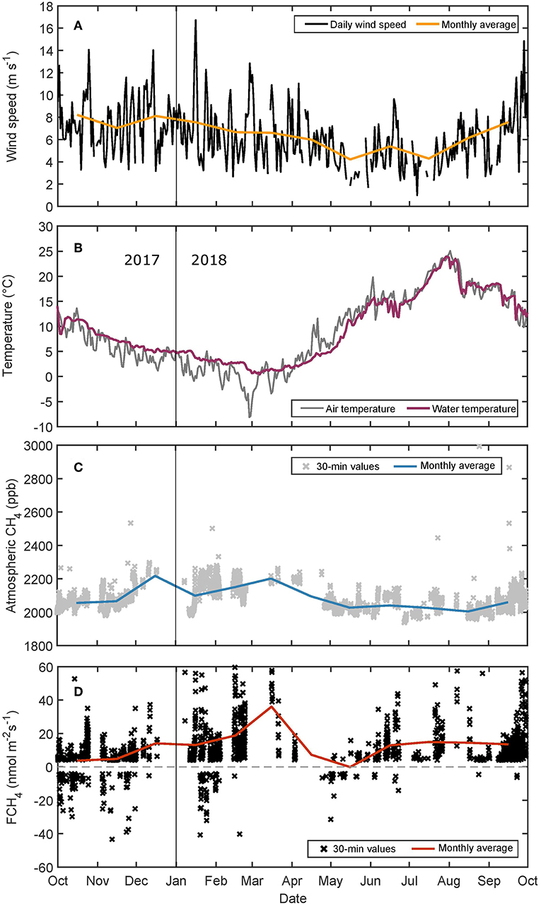
Figure 3. Annual cycle of (A) wind speed, (B) daily averages of air and water temperature, (C) 30-min and monthly averages of atmospheric CH₄ dry mole fraction, and (D) 30-min and monthly averages of air–sea FCH₄.

Air and water temperature presented a seasonal cycle with lower values during the winter months (DJFM) and higher temperatures during summer (JJAS). The air temperature monthly means ranged between 0.6°C and 5.4°C during winter, being February the coldest month. During summer, the monthly mean air temperatures ranged between 16.2°C and 22.7°C, being July the warmest month of the year. The water temperature showed a very similar behavior with a minimum monthly mean of 1.3°C in March and a maximum value of 19.3°C in July. The minimum air and water temperatures were -7.5°C and 0.4°C, respectively, and were both observed during late winter. The maximum air and water temperatures reached values of 27.2°C and 23.9°C, respectively. The mean annual air temperature was 10.2°C, while the mean annual water temperature was 9.4°C.

Higher values of the atmospheric CH₄ dry mole fraction were observed during winter compared to the values observed during the rest of the year. The maximum monthly mean was 2,217.7 ppb observed during December and a second maximum of 2,201.8 ppb occurred during March. Lower monthly values (~ 2,000 ppb) were found from April to November (Figure 3C). For FCH₄, positive monthly means were observed throughout the year with values of 3.7-36.1 nmol m⁻²s⁻¹ (excluding May) indicating that the region was a net source of CH₄. May was the only month with a negative monthly mean value of -0.1 nmol m⁻²s⁻¹. A maximum monthly mean of 36.0 nmol m⁻²s⁻¹ was observed during March. Additionally to this maximum value, high FCH₄ were observed both during winter and summer with similar monthly values ranging from 13.1 to 18.8 nmol m⁻²s⁻¹ and 12.9 to 14.9 nmol m⁻²s⁻¹, respectively. Minimum FCH₄ were observed during the transition months between summer and winter seasons, with near-zero fluxes during May and October-November. The scatter of the individual 30-min values was large ranging from -76 to 251.6 nmol m⁻²s⁻¹, with most of the negative values (163 out of 202 data points) observed during late autumn and winter.

3.1.1. Methane Concentrations: A Comparison With the MEMENTO Database

A comparison between the two datasets (Östergarnsholm data and MEMENTO) was carried out with the aim of understanding and validating the seasonal behavior observed from the EC measurements at Östergarnsholm. Monthly mean atmospheric CH₄ dry mole fraction observed from the EC measurements at Östergarnsholm during 2017-2018 ranged between 2,004.6 and 2,217.7 ppb, while the values previously reported in the MEMENTO database for the Gotland Basin region ranged from 1,860 to 1,905 ppb (Figure 4). Atmospheric values from the Gotland Basin included monthly averages over almost 30 years, excepting January for which no data was reported during those years. The long-term average showed a more clear seasonality, but it masked shorter-term changes and the higher variability observed in the 1-year record from Östergarnsholm. For both records, however, lower monthly CH₄ dry mole fractions were observed during summer (JJAS) with minimum values during August, 2,004.6 and 1,861.0 ppb, for Östergarnsholm and the Gotland Basin, respectively. Maximum values during November-April were observed also for both records.

FIGURE 4

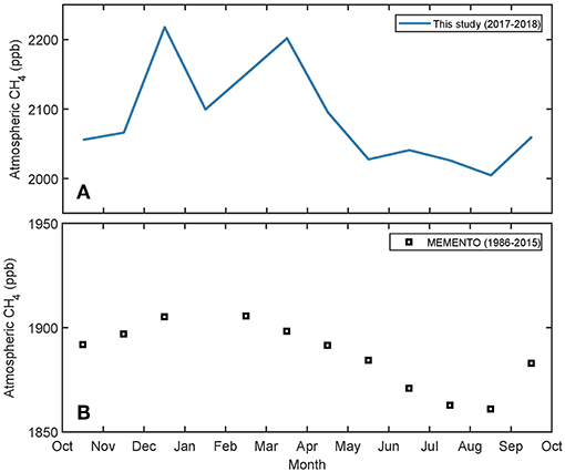
Figure 4. Monthly means of atmospheric CH₄ dry mole fraction from (A) Östergarnsholm station during 2017–2018 (this study), and (B) MEMENTO database in the Gotland Basin obtained between 1986 and 2015.

Similar to what was observed for the atmospheric concentrations, the CH₄ mole fractions in the seawater measured in the vicinities of the Östergarnsholm site were higher than the average values observed in the Gotland Basin (Figure 5). The mean value of the seawater CH₄ mole fraction from the 2-day mapping campaign in late June 2018 was 3,897.1 ppb, and the mean value from the discrete samplings in summer 2016 and 2017 was 8,794.1 ppb. On the contrary, the annual mean value reported for the Gotland Basin was 2,676.3 ppb, with higher values from late June to October, reaching a maximum monthly mean of 3,360.5 ppb in October. The mean values from the coastal regions—as defined above as “coastal” sub-dataset—reported in the MEMENTO database did not show either such high values as those reported within this study. Even so, individual values reaching magnitudes up to 15,000 ppb were reported (Figure 5), showing that under certain conditions, mostly during summer, high values of CH₄ in the seawater can occur in the region. During winter, lower values were observed from the MEMENTO data, the minimum value was found during May with monthly mean of 1,923.7 ppb. No data was reported during January.

FIGURE 5

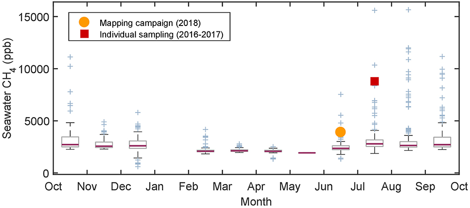
Figure 5. Boxplots representing the annual cycle of seawater CH₄ mole fractions in the Gotland Basin from the MEMENTO database. The yellow dot is the average value from the mapping campaign, and the red square is the mean value from the individual samplings. In the boxplots, the median value is represented by the purple line, the 25th and 75th percentiles indicated by the gray boxes, and outliers are marked as blue crosses.

A broader comparison using data from the whole Baltic Sea (Table 1) also supports that the magnitude of the seawater CH₄ mole fractions in the vicinities of the tower was much higher than values previously reported for the Baltic Sea (Figure 6). However, the measurements from the mapping campaign were in good agreement with values reported for the coastal regions. High-concentration events were observed for both the Baltic Sea and the coastal Baltic Sea datasets with values as high as 20,000 ppb.

FIGURE 6

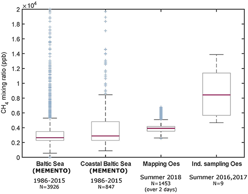
Figure 6. Boxplots of CH₄ mole fraction in the seawater. From left to right, the first two boxes represent data from MEMENTO database, the first one considers all data available for the Baltic Sea and the second one only data corresponding to regions with depth < 25 m, here defined as coastal Baltic Sea. The last two boxes represent data from the vicinities of Östergarnsholm site, where “Mapping Oes” shows results from the mapping campaign and “Ind. sampling Oes” the results of the individual sampling. “N” is the number of data points. The representation of the boxplots is the same as in Figure 5.

3.1.2. Seasonality of the Air-Sea Concentration Gradient

A clear seasonal pattern was observed in the air–sea concentration gradient of CH₄ (ΔC) from atmospheric and water-side CH₄ mole fractions in the Gotland Basin (Figure 7A). The gradient was, to a great extent, caused by changes in the water-side mole fractions while atmospheric CH₄ remained fairly constant. The increase in the seawater mole fractions led to higher positive ΔC that reached values higher than 1,000 ppb during summer and early autumn. The maximum values were found in September and October when the ΔC values were higher than 1,460 ppb. The FCH₄ values observed from Östergarnsholm data during the summer months were consistent with the behavior of ΔC, showing an increase during these months (Figure 7B). In the same way, the minimum ΔC of 39.4 ppb during May was in agreement with the minimum FCH₄ when a near-zero flux was observed. During the winter months ΔC was small, even so, we observed high FCH₄, suggesting that other processes might have modulated the air–sea fluxes by enhancing the efficiency of the transport through the surface.

FIGURE 7

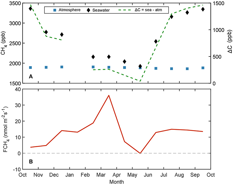
Figure 7. (A) Annual cycle of seawater and atmospheric CH₄ mole fractions (principal y-axis) and mole fraction gradient (ΔC = C_seawater - C_atmosphere) (secondary y-axis); data corresponding to the Gotland Basin from MEMENTO database (1986-2015). (B) Annual cycle of air–sea CH₄ flux (FCH₄) calculated from EC.

3.2. Wind Dependency

Slightly soluble gases tend to be more easily transported across the air–sea interface under highly turbulent conditions (bubble-mediated transport). Based on the mean values (blue dots in Figure 8) such correlation between FCH₄ and the wind speed (U) was not noticeable. For high-wind speed values (U > 14 m s⁻¹) a tendency of FCH₄ to increase with wind speed was observed. However, these values had been identified to belong to a single high-wind speed event (see section 3.2.1) and further evidence is required to validate the relationship between FCH₄ under high-wind speeds.

FIGURE 8

Figure 8. Half-hourly FCH₄ values plotted as a function of the wind speed, U.

When comparing FCH₄ as a function of the wind speed, several parameters affecting the flux were included in the comparison. A more fair comparison would be to represent the transfer velocity (k) as a function of U since FCH₄ is not only influenced by the U but also by ΔC. Unfortunately, we were not able to calculate k in this study due to the lack of continuous measurements of CH₄ mole fractions in the seawater.

3.2.1. High-Wind Speed Event

A high-wind speed event occurred in January 2018, the case is here highlighted as it revealed a strong wind speed dependence for FCH₄. This event is particularly interesting for further analysis since it occurred during winter when ΔC is assumed to be small, therefore, is unlikely the main driver of FCH₄.

During the high-wind speed event, a constant increase of the wind speed occurred over a 48-h period (Figure 9A). The initial wind speed at the beginning of the event was 5.1 m s⁻¹ and steadily increased until it reached its maximum at 19.4 m s⁻¹ almost 48 h later. The wind direction during the event was from south-east, with mean wind direction of 154°. South-east wind directions represent open sea conditions as defined by Rutgersson et al. (2008). We observed an increase of FCH₄ several hours after the event began (Figure 9B). During the high-wind speed event, FCH₄ increased exponentially from an initial value of 4.0 nmol m⁻² s⁻¹ to a maximum value of 187.1 nmol m⁻² s⁻¹. Additional to the increase in FCH₄, an increment on the atmospheric CH₄ dry mole fraction was observed from an initial value of 2,006.1 ppb to a maximum value of 2,438.2 ppb.

FIGURE 9

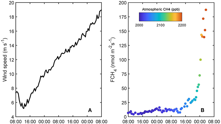
Figure 9. (A) Wind speed, and (B) air–sea FCH₄ over a 48-h period during a high-wind speed event in January 14–16, 2018. The starting date is January 14 at 8:00 UTC, and the ending time is January 16 at 8:00 UTC.

4. Discussion

The annual cycle of atmospheric CH₄ dry mole fraction observed at Östergarnsholm station showed a good agreement with the seasonal variability of the Gotland Basin from previously reported data, lower atmospheric CH₄ values were observed during summer and higher values during winter time. The seasonal variability observed in both datasets might be explained by the increased consumption rate of CH₄ in the atmosphere due to OH radicals during summer (Khalil and Rasmussen, 1983). The magnitude of the monthly means observed during 2017-2018 at Östergarnsholm were significantly higher than the values presented for the Gotland Basin (Figure 4). To our knowledge there is no other continuous atmospheric CH₄ measurements in the region to compare with, however, the values from the Östergarnsholm station seem to be consistent with the global trends that indicate an increase of about 200 ppb in the global atmospheric CH₄ concentration since 1985 (Figure 1 in Saunois et al., 2016). Additionally, higher air–sea FCH₄ enhanced by coastal processes might also contribute to the observed atmospheric values. Higher variability is observed in the monthly means from the EC measurements of atmospheric CH₄. The variability is attributed to local processes which were not perceptible from the long-term averages in the Gotland Basin form the MEMENTO data. Even so, more data is still necessary to validate the measurements presented here and to explain the high variability on the atmospheric CH₄ mole fraction.

The CH₄ mole fractions in the seawater nearby the Östergarnsholm site were higher than both the mean and median values from measurements reported in the MEMENTO database for the Gotland Basin (Figure 5). However, similar values have been observed in the region during summer time. These results are consistent with the seasonal temperature cycle which enhances the CH₄ production rate under warmer water conditions (Bange et al., 1998). Additionally, Gülzow et al. (2013) showed that upwelling events during the summer have a significant effect on surface CH₄ on the Gotland area by bringing CH₄-rich water masses from deeper layer to the surface.

The water-side measurements at Östergarnsholm were in good agreement with values reported for the coastal Baltic Sea regions (Figure 6), suggesting that coastal characteristics such as shallow waters, high biological activity, and upwelling events might have led to higher concentration values in the vicinities of the tower. High water-side CH₄ mole fractions have been previously reported for physical- and biogeochemically active areas such as coastal regions (Rhee et al., 2009; Borges et al., 2016) and lakes (Podgrajsek et al., 2014). Borges et al. (2016) attributed the high CH₄ concentrations observed in a near-shore region in the North Sea—and the consequent fluxes—to the shallow water-depth and the well-mixed water column. Gülzow et al. (2013) concluded that for other shallow areas in the Baltic Sea (i.e., Mecklenburg Bight and Arkona Basin) the methane oversaturation conditions follow the water temperature trend, with increasing concentrations during summer time. This fact is particularly relevant as 2018 presented significantly higher water temperatures than average years.

The monthly means of FCH₄ from EC measurements at Östergarnsholm site indicated that the region was a net source of CH₄ throughout the year. The role of the Baltic Sea as a source of CH₄ has been mentioned in previous studies, however, the reported values present a great degree of variability in time and space. On one hand, Bange et al. (1994) reported values ranging from 0.11 to 0.17 nmol m⁻²s⁻¹ during a winter (February) and from 1.17 to 13.9 nmol m⁻²s⁻¹ for the summer (July/August), indicating larger flux during summer than during winter. On the other hand, Gülzow et al. (2013) showed that the seasonality of FCH₄ depends on the characteristics of each region of the Baltic Sea. The fluxes calculated by Gülzow et al. (2013) are significantly smaller than those presented by Bange et al. (1994); for the same months they found values of 0.151-0.08 nmol m⁻²s⁻¹ (February) and 0.01-0.076 nmol m⁻²s⁻¹ (July/August) for the Arkona Sea, Bornholm Sea, and Gotland Sea. The highest monthly mean value reported by Gülzow et al. (2013) was 1.145 nmol m⁻²s⁻¹ in the Gulf of Finland during February. In both cases, the fluxes were calculated based on bulk parameterizations.

The FCH₄ monthly means presented in this study ranged from -0.1 to 36.1 nmol m⁻²s⁻¹ from EC measurements. These values are—in general—higher than those previously reported for the Baltic Sea. In a similar way, De Wilde and Duyzer (1995) reported FCH₄ values from the ASGASEX experiment up to 6 times higher using micrometeorological techniques than those calculated using Wanninkhof (1992) relationship. The authors mentioned that in order to explain those discrepancies between the two methods, more measurements are required using both methods simultaneously.

Despite the positive mean fluxes throughout the year and the general agreement of the Baltic Sea as a net source of CH₄, some negative FCH₄ values were observed from the 30-min data during late autumn and winter (Figure 3D). These values might have been caused by a temporary undersaturation of the water-side CH₄ with respect of the atmospheric values. Gülzow et al. (2013) calculated saturation values of 96% and 94% during winter in 2010 and 2011, respectively, in the Gotland Basin. The undersaturation was only reported for the Goltand Basin region during December-April and might be caused by the enhanced solubility of CH₄ due to low water temperatures. Thus, this behavior is not noticeable from the mole fraction time series (Figure 3C), however, it might cause frequent changes in the direction of the net FCH₄ in the region. In addition to the possibility of a temporary undersaturation state, highly turbulent conditions due to increased wind speeds during winter time may cause higher variability on the gas exchange across the interface, the direction of FCH₄ is then determined by the air-sea gradient. High temporal resolution measurements, such as those presented here, are necessary to detect this variability.

In the Gotland Basin, ΔC is mostly modulated by variations of CH₄ mole fraction in the seawater, while the atmospheric values remain relatively constant in comparison to the seawater values. From the MEMENTO data, it was noticeable that higher ΔC values are present during summer (Figure 7) due to the large increase in the seawater mole fractions observed in the warmer months. Similarly, Gülzow et al. (2013) observed a continuous increase of CH₄ saturation in all basins of the Baltic Sea from April to July due to the rise in water temperatures. The MEMENTO data is useful for describing the average seasonal behavior, however, sub-annual variability of ΔC for the particular period of this study is hardly represented. In order to understand the relationship between ΔC and the fluxes across the air-sea interface, simultaneous measurements of atmospheric and seawater concentrations are required, along with flux data.

In this study, FCH₄ values observed during the summer months (JJAS) were consistent with the increase of ΔC as observed from the MEMENTO data, suggesting that the main driver of the exchange is the air–water concentration difference. In this case, the effect of the strong stratification and shallow mixed layer depth in the Gotland Basin (Gülzow et al., 2013) during the summer due to the warming of the surface layers is not sufficient to hinder FCH₄, at least in this particular region. In contrast, high FCH₄ observed during winter were not explained solely by ΔC that showed small values from October to May. During winter, strong wind-speed events and higher mean wind speed values were observed. Regardless of the relatively small gradient, highly-turbulent conditions might have led to the enhancement of the transport processes causing an increase in positive FCH₄.

Air–sea gas exchange is not only dependent on ΔC, it is also modulated by environmental forcing factors that define the efficiency of the transport (Wanninkhof et al., 2009). Wind speed is considered to be one of the main parameters used to describe the efficiency of the gas exchange across the air–sea interface (Liss and Merlivat, 1986; Wanninkhof, 1992). Thus, a high correlation between FCH₄ and U was expected, however, no correlation was observed between the calculated FCH₄ and U (Figure 8). We considered that using k would be a more straightforward comparison. Gülzow et al. (2013) presented values of k for different regions of the Baltic Sea calculated according to Wanninkhof et al. (2009) as a function of the wind speed. They showed that for all regions (including the Gotland Basin) the highest transfer coefficients occurred from September to January. These results are consistent with the increased wind speeds observed in this study during the winter months, and can be an indication of the high FCH₄ values observed during this period might be driven by wind-induced turbulence.

The analysis of a high-wind speed event showed that under certain conditions the wind speed might be a crucial parameter in the gas transport across the air-sea interface causing an increase in FCH₄. In the Baltic Sea, CH₄ is primarily produced in the sediments and then transported through the water column, therefore, the physical characteristics on the water-side (i.e., stratification, tides, mixed layer depth, etc.) are of great importance for the distribution of CH₄. However, high-wind speed events—such as the one analyzed here—can cause enough mixing to ventilate the water column enhancing the transport of CH₄ to the atmosphere, resulting in larger positive FCH₄. The delay on the increasing behavior of FCH₄ and CH₄ dry mole fraction during the high-wind speed event, suggests the existence of a threshold value below which the wind does not generate enough mixing. Alternatively, this behavior might be an indication of the need for a sufficiently-long time over which the wind develops the mixing in the ocean surface. Bell et al. (2017) showed that the effect of the bubble-mediated transport at intermediate-high wind speeds becomes significant after a threshold value that depends on the wave-breaking characteristics. The threshold value was found to be dependent on the characteristics of the gas. Analysis of the effect of bubble-mediated transport on FCH₄ is still missing. High-wind speed events are difficult to capture both by water and atmospheric measurements since they are sporadic and the strong weather conditions might limit the possibility of sampling.

Based on the results presented in this study, we show that high frequency measurements of CH₄ are a useful tool for direct flux estimations in the marine environment if the technical limitations are overcome. This technique can supply information about the net transport of the gas across the air-sea interface without using parameterizations. However, strict quality control criteria are required to ensure the good quality of the data and the fulfillment of the EC requirements. Long-term CH₄ data from Östergarnsholm station could be used along with other monitoring infrastructures to establish the methane budgets in the Baltic Sea.

5. Conclusions

Air-sea FCH₄ calculated in this study using the EC method are, to our best knowledge, the first continuous measurements of FCH₄ in the Baltic Sea. We present 1 year of direct FCH₄ using EC measurements from the land-based station at Östergarnsholm site. The annual cycle of FCH₄ seems to be controlled by the seasonality of ΔC, which at the same time is mostly modulated by the seawater concentrations. Further analysis of the impact of ΔC on FCH₄ based on simultaneous measurements is still required. Additionally, the wind seems to play an important role on the CH₄ gas exchange under high wind speed conditions.

The results presented here support previous analyses suggesting that the coastal regions are highly active areas that can contribute to a great extent to the oceanic CH₄ emissions. Small availability of CH₄ data in the marine environment is the main restriction to better understand of the processes involved on air-sea CH₄ exchange. Therefore, we suggest the use of EC measurements for the estimation and monitoring of FCH₄ in the marine environment. EC measurements can contribute to the analysis of the mechanisms controlling the air-sea gas exchange, to establish regional carbon and methane budgets in the Baltic Sea, and to improve parameterizations of the gas transfer velocity in the region.

Author Contributions

LG-L and MW participated in the installation and continuous maintenance of the instruments. AR conceived the idea and initial planning of the study. LG-L analyzed the data. EN developed part of the data treatment procedure and quality control. AR, ES, and MW participated in the interpretation of the results and contributed with the outline of the manuscript. LG-L wrote the article. HB and AK provided the MEMENTO data and contributed with the analysis and discussion of water-side data. All the co-authors participated in the discussion of results and revision of the article.

Funding

The BONUS INTEGRAL project receives funding from BONUS (Art 185), funded jointly by the EU, the Swedish Research Council Formas, the Academy of Finland, the Estonian Research Council, the Polish National Centre for Research and Development, and the German Federal Ministry of Education and Research. The ICOS station Östergarnsholm is funded by the Swedish Research Council (grants 2012-03902 and 2013-02044) and Uppsala University.

Conflict of Interest Statement

The authors declare that the research was conducted in the absence of any commercial or financial relationships that could be construed as a potential conflict of interest.

Acknowledgments

The authors would like to thank the two reviewers for their constructive comments and suggestions that contributed to improving this manuscript.

This work forms part of the BONUS INTEGRAL project.

References

Aubinet, M., Vesala, T., and Papale, D. (2012). Eddy Covariance: A Practical Guide to Measurement and Data Analysis. London; New York, NY; Dordrecht; Heidelberg: Springer.

Google Scholar

Baldocchi, D., Falge, E., Gu, L., Olson, R., Hollinger, D., Running, S., et al. (2001). FLUXNET: a new tool to study the temporal and spatial variability of ecosystem-scale carbon dioxide, water vapor, and energy flux densities. Bull. Amer. Meteorol. Soc. 82, 2415–2434. doi: 10.1175/1520-0477(2001)082<2415:FANTTS>2.3.CO;2

CrossRef Full Text | Google Scholar

Baldocchi, D. D., Detto, M., Sonnentag, O., Verfaillie, J., Teh, Y. A., Silver, W., et al. (2012). The challenges of measuring methane fluxes and concentrations over a peatland pasture. Agricult. For. Meteorol. 153, 177–187. doi: 10.1016/j.agrformet.2011.04.013

CrossRef Full Text | Google Scholar

Baldocchi, D. D., Hincks, B. B., and Meyers, T. P. (1988). Measuring biosphere-atmosphere exchanges of biologically related gases with micrometeorological methods. Ecology 69, 1331–1340. doi: 10.2307/1941631

CrossRef Full Text | Google Scholar

Bange, H. W. (2006). Nitrous oxide and methane in European coastal waters. Estuar. Coast. Shelf Sci. 70, 361–374. doi: 10.1016/j.ecss.2006.05.042

CrossRef Full Text | Google Scholar

Bange, H. W., Bartell, U. H., Rapsomanikis, S., and Andreae, M. O. (1994). Methane in the Baltic and North Seas and a reassessment of the marine emissions of methane. Glob. Biogeochem. Cycles 8, 465–480. doi: 10.1029/94GB02181

CrossRef Full Text | Google Scholar

Bange, H. W., Bergmann, K., Hansen, H. P., Kock, A., Koppe, R., Malien, F., et al. (2010). Dissolved methane during hypoxic events at the Boknis Eck time series station (Eckernförde Bay, SW Baltic Sea). Biogeosciences 7, 1279–1284. doi: 10.5194/bg-7-1279-2010

CrossRef Full Text | Google Scholar

Bange, H. W., Dahlke, S., Ramesh, R., Meyer-Reil, L.-A., Rapsomanikis, S., and Andreae, M. O. (1998). Seasonal study of methane and nitrous oxide in the coastal waters of the southern Baltic Sea. Estuar. Coast. Shelf Sci. 47, 807–817. doi: 10.1006/ecss.1998.0397

CrossRef Full Text | Google Scholar

Bell, T. G., Landwehr, S., Miller, S. D., Bruyn, W. J. D., Callaghan, A. H., Scanlon, B., et al. (2017). Estimation of bubble-mediated air–sea gas exchange from concurrent DMS and CO₂ transfer velocities at intermediate–high wind speeds. Atmospher. Chem. Phys. 17, 9019–9033. doi: 10.5194/acp-17-9019-2017

CrossRef Full Text | Google Scholar

Borges, A. V., Champenois, W., Gypens, N., Delille, B., and Harlay, J. (2016). Massive marine methane emissions from near-shore shallow coastal areas. Sci. Rep. 6:27908. doi: 10.1038/srep27908(2016)

PubMed Abstract | CrossRef Full Text | Google Scholar

Brock, F. V. (1986). A nonlinear filter to remove impulse noise from meteorological data. J. Atmospher. Ocean. Technol. 3, 51–58. doi: 10.1175/1520-0426(1986)003<0051:ANFTRI>2.0.CO;2

CrossRef Full Text | Google Scholar

Crawford, T. L., McMillen, R. T., Meyers, T. P., and Hicks, B. B. (1993). Spatial and temporal variability of heat, water vapor, carbon dioxide, and momentum air–sea exchange in a coastal environment. J. Geophys. Res. 98, 12869–12880. doi: 10.1029/93JD00628

CrossRef Full Text | Google Scholar

De Wilde, H. P. J., and Duyzer, J. (1995). “Methane emissions off the Dutch coast: air-sea concentration differences versus atmospheric gradients,” in Third International Symposium on Air-Water Gas Transfer (Heidelberg), 763–773.

Google Scholar

Detto, M., Verfaillie, J., Anderson, F., Xu, L., and Baldocchi, D. (2011). Comparing laser-based open-and closed-path gas analyzers to measure methane fluxes using the eddy covariance method. Agricult. For. Meteorol. 151, 1312–1324. doi: 10.1016/j.agrformet.2011.05.014

CrossRef Full Text | Google Scholar

Foken, T. (2008). Micrometeorology. Berlin; Heidelberg: Springer-Verlag.

Google Scholar

Fowler, D., and Duyzer, J. H. (1989). “Micrometeorological techniques for the measurement of trace gas exchange,” in Exchange of Trace Gases between Terrestrial Ecosystems and the Atmosphere, Dahlem Workshop Report, Life Science Research Reports 47, eds Andreae, M. O. and Schimel, D. S. (Berlin: Wiley Interscience), 189–208.

Google Scholar

Gülzow, W., Gräwe, U., Kedzior, S., Schmale, O., and Rehder, G. (2014). Seasonal variation of methane in the water column of Arkona and Bornholm Basin, western Baltic Sea. J. Mar. Syst. 139, 332–347. doi: 10.1016/j.jmarsys.2014.07.013

CrossRef Full Text | Google Scholar

Gülzow, W., Rehder, G., Schneider von Deimling, J., Seifert, S., and Tóth, Z. (2013). One year of continuous measurements constraining methane emissions from the Baltic Sea to the atmosphere using a ship of opportunity. Biogeosciences 10, 81–99. doi: 10.5194/bg-10-81-2013

CrossRef Full Text | Google Scholar

Gülzow, W., Rehder, G., Schneider, B., von Deimling, J. S., and Sadkowiak, B. (2011). A new method for continuous measurement of methane and carbon dioxide in surface waters using off-axis integrated cavity output spectroscopy (ICOS): an example from the Baltic Sea. Limnol. Oceanogr. 9, 176–184. doi: 10.4319/lom.2011.9.176

CrossRef Full Text | Google Scholar

Gutiérrez-Loza, L., Ocampo-Torres, F. J., and García-Nava, H. (2018). The effect of breaking waves on CO₂ air–sea fluxes in the coastal zone. Boundary Layer Meteorol. 168, 343–360. doi: 10.1007/s10546-018-0342-x

CrossRef Full Text | Google Scholar

Högström, U., Sahlée, E., Drennan, W. M., Kahma, K. K., Smedman, A.-S., Johansson, C., et al. (2008). Momentum fluxes and wind gradients in the marine boundary layer: a multi platform study. Boreal Environ. Res. 13, 475–502.

Google Scholar

IPCC (2013). Climate change 2013: The Physical Science Basis. Contribution of Working Group I to the Fifth Assessment Report of the Intergovernmental Panel on Climate Change. Cambridge: Cambridge University Press.

Google Scholar

Khalil, M. A. K., and Rasmussen, R. A. (1983). Sources, sinks, and seasonal cycles of atmospheric methane. J. Geophys. Res. 88, 5131–5144. doi: 10.1029/JC088iC09p05131

CrossRef Full Text | Google Scholar

Liss, P. S., and Merlivat, L. (1986). “Air–sea gas exchange rates: introduction and synthesis,” in The Role of Air–Sea Exchange in Geochemical Cycling (Dordrecht: Springer), 113–127.

Google Scholar

McDermitt, D., Burba, G., Xu, L., Anderson, T., Komissarov, A., Riensche, B., et al. (2011). A new low-power, open-path instrument for measuring methane flux by eddy covariance. Appl. Phys. B 102, 391–405. doi: 10.1007/s00340-010-4307-0

CrossRef Full Text | Google Scholar

McGillis, W. R., Edson, J. B., Hare, J. E., and Fairall, C. W. (2001). Direct covariance air-sea CO₂ fluxes. J. Geophys. Res. 106, 16729–16745. doi: 10.1029/2000JC000506

CrossRef Full Text | Google Scholar

Meier, H. E. M., Rutgersson, A., and Reckermann, M. (2014). An earth system science program for the Baltic Sea region. Eos Trans. Amer. Geophys. Union 95, 109–110. doi: 10.1002/2014EO130001

CrossRef Full Text | Google Scholar

Miller, S. D., Marandino, C., and Saltzman, E. S. (2010). Ship-based measurement of air–sea CO₂ exchange by eddy covariance. J. Geophys. Res. 115, 1–14. doi: 10.1029/2009JD012193

CrossRef Full Text | Google Scholar

Paranaíba, J. R., Barros, N., Mendonça, R., Linkhorst, A., Isidorova, A., Roland, F., et al. (2018). Spatially resolved measurements of CO₂ and CH₄ concentration and gas-exchange velocity highly influence carbon-emission estimates of reservoirs. Environ. Sci. Technol. 52, 607–615. doi: 10.1021/acs.est.7b05138

PubMed Abstract | CrossRef Full Text | Google Scholar

Podgrajsek, E., Sahlée, E., Bastviken, D., Natchimuthu, S., Kljun, N., Chmiel, H. E., et al. (2016). Methane fluxes from a small boreal lake measured with the eddy covariance method. Limnol. Oceanogr. 61, S41–S50. doi: 10.1002/lno.10245

CrossRef Full Text | Google Scholar

Podgrajsek, E., Sahlée, E., and Rutgersson, A. (2014). Diurnal cycle of lake methane flux. J. Geophys. Res. 119, 236–248. doi: 10.1002/2013JG002327

CrossRef Full Text | Google Scholar

Rhee, T. S., Kettle, A. J., and Andreae, M. O. (2009). Methane and nitrous oxide emissions from the ocean: a reassessment using basin-wide observations in the Atlantic. J. Geophys. Res. 114, 1–20. doi: 10.1029/2008JD011662

CrossRef Full Text | Google Scholar

Rutgersson, A., Norman, M., Schneider, B., Pettersson, H., and Sahlée, E. (2008). The annual cycle of carbon dioxide and parameters influencing the air–sea carbon exchange in the Baltic Proper. J. Mar. Syst. 74, 381–394. doi: 10.1016/j.jmarsys.2008.02.005

CrossRef Full Text | Google Scholar

Rutgersson, A., and Smedman, A.-S. (2010). Enhanced air–sea CO₂ transfer due to water-side convection. J. Mar. Syst. 80, 125–134. doi: 10.1016/j.jmarsys.2009.11.004

CrossRef Full Text | Google Scholar

Sahlée, E., Rutgersson, A., Podgrajsek, E., and Bergström, H. (2014). Influence from surrounding land on the turbulence measurements above a lake. Boundary layer Meteorol. 150, 235–258. doi: 10.1007/s10546-013-9868-0

CrossRef Full Text | Google Scholar

Sahlée, E., Smedman, A. S., Högström, U., and Rutgersson, A. (2008). Reevaluation of the bulk exchange coefficient for humidity at sea during unstable and neutral conditions. J. Phys. Oceanogr. 38, 257–272. doi: 10.1175/2007JPO3754.1

CrossRef Full Text | Google Scholar

Saunois, M., Bousquet, P., Poulter, B., Peregon, A., Ciais, P., Canadell, J. G., et al. (2016). The global methane budget 2000-2012. Earth Syst. Sci. Data 8:697. doi: 10.5194/essd-8-697-2016

CrossRef Full Text | Google Scholar

Schmale, O., Von Deimling, J. S., Gülzow, W., Nausch, G., Waniek, J. J., and Rehder, G. (2010). Distribution of methane in the water column of the Baltic Sea. Geophys. Res. Lett. 37, 1–5. doi: 10.1029/2010GL043115

CrossRef Full Text | Google Scholar

Schmaljohann, R. (1996). Methane dynamics in the sediment and water column of Kiel Harbour (Baltic Sea). Mar. Ecol. Prog. Ser. 131, 263–273. doi: 10.3354/meps131263

CrossRef Full Text | Google Scholar

Smedman, A. S., Högström, U., Bergström, H., Rutgersson, A., Kahma, K. K., and Pettersson, H. (1999). A case study of air–sea interaction during swell conditions. J. Geophys. Res. 104, 25833–25851. doi: 10.1029/1999JC900213

CrossRef Full Text | Google Scholar

Starkenburg, D., Metzger, S., Fochesatto, G. J., Alfieri, J. G., Gens, R., Prakash, A., et al. (2016). Assessment of despiking methods for turbulence data in micrometeorology. J. Atmospher. Ocean. Technol. 33, 2001–2013. doi: 10.1175/JTECH-D-15-0154.1

CrossRef Full Text | Google Scholar

Vickers, D., and Mahrt, L. (1997). Quality control and flux sampling problems for tower and aircraft data. J. Atmospher. Ocean. Technol. 14, 512–526. doi: 10.1175/1520-0426(1997)014<0512:QCAFSP>2.0.CO;2

CrossRef Full Text | Google Scholar

Wanninkhof, R. (1992). Relationship between gas exchange and wind speed over the ocean. J. Geophys. Res. 97, 7373–7381. doi: 10.1029/92JC00188

CrossRef Full Text | Google Scholar

Wanninkhof, R., Asher, W. E., Ho, D. T., Sweeney, C., and McGillis, W. R. (2009). Advances in quantifying air-sea gas exchange and environmental forcing. Ann. Rev. Mar. Sci. 1, 213–244. doi: 10.1146/annurev.marine.010908.163742

PubMed Abstract | CrossRef Full Text | Google Scholar

WDCGG. (2015). Data Summary No. 39. Volume IV-Greenhouse Gases and Other Atmospheric Gases. Japan Meteorological Agency, World Meteorological Organization.

Google Scholar

Webb, E. K., Pearman, G. I., and Leuning, R. (1980). Correction of flux measurements for density effects due to heat and water vapour transfer. Q. J. R. Meteorol. Soc. 106, 85–100. doi: 10.1002/qj.49710644707

CrossRef Full Text | Google Scholar

Wiesenburg, D. A., and Guinasso, N. L. (1979). Equilibrium solubilities of methane, carbon monoxide, and hydrogen in water and sea water. J. Chem. Eng. Data 24, 356–360. doi: 10.1021/je60083a006

CrossRef Full Text | Google Scholar

Yang, M., Bell, T. G., Brown, I. J., Fishwick, J. R., Kitidis, V., Nightingale, P. D., et al. (2019). Insights from year-long measurements of air-water CH₄ and CO₂ exchange in a coastal environment. Biogeosciences 16, 961–978. doi: 10.5194/bg-16-961-2019

CrossRef Full Text | Google Scholar

Yang, M., Bell, T. G., Hopkins, F. E., Kitidis, V., Cazenave, P. W., Nightingale, P. D., et al. (2016a). Air–sea fluxes of CO₂ and CH₄ from the Penlee Point Atmospheric Observatory on the south-west coast of the UK. Atmospher. Chem. Phys. 16, 5745–5761. doi: 10.5194/acp-16-5745-2016

CrossRef Full Text | Google Scholar

Yang, M., Prytherch, J., Kozlova, E., Yelland, M. J., Parenkat Mony, D., and Bell, T. G. (2016b). Comparison of two closed-path cavity-based spectrometers for measuring air–water CO₂ and CH₄ fluxes by eddy covariance. Atmospher. Meas. Techniq. 9, 5509–5522. doi: 10.5194/amt-9-5509-2016

CrossRef Full Text | Google Scholar