Age-Heterogeneity in Marine Sediments Revealed by Three-Dimensional High-Resolution Radiocarbon Measurements

1 Introduction

Proxy data from climate archives have been used for decades to reconstruct climate beyond the instrumental period. The information of past temperatures is, for example, stored in the δ¹⁸O and the Mg/Ca-ratio in calcite shells of organisms (e.g. foraminifera) embedded in marine sediments (e.g. Nürnberg et al., 1996; Lea, 2014). These shells are produced in the water column, rain down on the ocean seafloor, accumulate over time and build a continuous archive with deeper layers representing earlier times. For the interpretation of the recorded environmental parameters via paleoclimate proxies, a reliable conversion from depth to age is necessary. For material from the past 55,000 years, the measured radiocarbon content can be interpreted as a tracer of time since deposition (Libby et al., 1949; Blaauw and Heegaard, 2012; Heaton et al., 2021). To this end, the ratio of ¹⁴C/¹²C (in the following, we only refer to ¹⁴C) of carbon-containing sedimentary material, e.g. the calcite shell of foraminifera, is typically measured from several depth layers along a sediment core. These discrete age estimates are then interpolated by applying statistical methods to obtain a continuous depth-age scale for the entire sedimentary archive (Bard et al., 1987; Ramsey, 2008; Blaauw and Christen, 2011).

In oxygenated sediments that form the bulk of the marine sedimentary archives used for paleoclimate reconstruction, the deposited material is mixed by burrowing and feeding activities of the benthic fauna in the upper layer of sediment (Berger et al., 1979; Savrda and Bottjer, 1991; Casanova-Arenillas et al., 2022). As the rate of biological mixing, i.e. the bioturbation, is usually large compared to the sediment accumulation rate, the sediment becomes well mixed before it is eventually buried below the mixed layer (Figure 1A) (Berger and Heath, 1968). This mixing considerably modifies the sequence of recorded environmental properties and a down-core proxy time series represents only a smoothed version of the true climatic and temporal history (Goreau, 1980; Schiffelbein and Hills, 1984; Bard et al., 1987). Sediments from the same depth layer therefore contain a mixture of relocated younger and older material which complicates the interpretation of proxy variables, as well as the determination of the age of a sediment layer; the latter because measurements are performed on a finite number of specimens which may not be representative of the true mean age and proxy value of the layer (e.g. Lougheed et al., 2018; Dolman et al., 2021a).

FIGURE 1

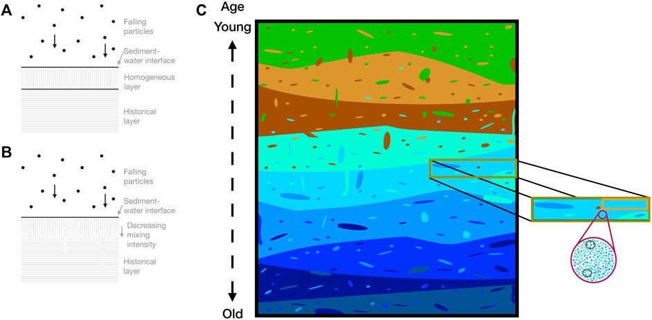
FIGURE 1. Conceptual sketches of mixing processes and sediment heterogeneity in a marine environment. Following the traditional terms of the mixed and the historical layer, (A) shows a well-defined boundary between both layers while (B) shows more dynamic mixing processes including deep reaching burrows. (C) illustrates a potential two-dimensional view of the heterogeneous distribution of consistently increasing ages with depth. The panels on the right hand side show a zoom into local age-heterogeneity. Colored dots and areas indicate marks from mixing of fine materials, fossils and other detrital components.

Simple quantitative descriptions of the mixing (Berger and Heath, 1968; Berger and Killingley, 1982) assume a complete and instantaneous mixing of the sediment down to a fixed depth, and no further mixing below (Figure 1A). Under this assumption, the degree of smoothing affecting the archived climate record and the expected variations between age-determinations from different samples from the same sediment layer are well studied (e.g. Goreau, 1980; Dolman et al., 2021a).

In reality, the intensity of mixing might vary which would lead to non-uniform and incomplete mixing. Furthermore, secondary modifications by trace fossils of different sizes, such as Chondrites, Planolites, Thalassinoides, Scolicia, and Zoophycos, result in vertical and horizontal variability as well (Figures 1B,C) (e.g. Dorador et al., 2020; Casanova-Arenillas et al., 2022). The impacts within the sediment are deep-reaching burrows and spreiten with fillings different from the surrounding sediment leading to considerable horizontal differences in age estimates on local (intra-sample, mm-to cm-scale) and regional (between different samples and cores, m-to km-scale) spatial scales (Anderson, 2001; Bard, 2001; Löwemark and Werner, 2001; Lougheed et al., 2020). These post-depositional modifications can be visualized and analyzed with X-ray images highlighting the magnitude of sediment heterogeneity (e.g. Löwemark and Werner, 2001; Löwemark et al., 2008; Trauth, 2013).

For a quantitative use of paleoclimate records, especially for large-scale compilations (e.g. Marcott et al., 2013), model-data comparisons (e.g. Laepple and Huybers, 2014) or data assimilation (e.g. Osman et al., 2021), the uncertainties and distortions in the proxy record and age-model have to be known. Here, proxy-system models (Evans et al., 2013; Dee et al., 2017; Dolman and Laepple, 2018) or analytical error models (Kunz et al., 2020; Dolman et al., 2021b) can be used if the processes contributing to the signal formation are known. Analyzing global compilations of Holocene and Glacial marine records, Reschke et al. (2019a,b) showed that the correlation of nearby proxy records is very low compared to the expectations from climate models, and that this cannot be explained by the classical age model uncertainty estimates derived from radiocarbon measurement and calibration. One hypothesis for this low correlation is that the true uncertainty of the age model may be larger due to heterogeneity in the sediment. Such a strong effect of archive heterogeneity was previously found in other climate archive types, e.g. ice cores from polar ice-sheets (Münch and Laepple, 2018).

In the quest of a full characterization of sediment mixing and age uncertainty, recent developments of ultra-small sample radiocarbon dating techniques (e.g. <100 μg CaCO₃) provide an important tool. They allow the measurement of the age of individual or small numbers (<10) of specimens (Wacker et al., 2010, 2013). This information can be used to quantify the within-sample variability, i.e. the spread between the youngest and the oldest material, at one depth (Lougheed et al., 2018; Fagault et al., 2019; Lougheed et al., 2020; Dolman et al., 2021a).

Here we characterize the heterogeneity and the factors contributing to the age uncertainty of sedimentary archives by generating radiocarbon data using nine replicate cores extracted from a single boxcore, thereby affording a 3-dimensional view on the ¹⁴C variability within a 24 × 24 × 34 cm volume. This allows us to estimate the bioturbational mixing and the sediment heterogeneity and to infer the full age model uncertainty accounting for these effects. Finally, we discuss possible implications of the age-heterogeneity on paleo reconstructions and provide suggestions for an optimal sampling scheme targeted to bioturbated sediments.

2 Methods

2.1 Study Approach

To quantify and characterize the sediment heterogeneity affecting paleo-environmental reconstructions from marine archives, we study an oxygenated marine sediment core retrieved from the southern South China Sea using a box corer (Figure 2A, 10° 54.0262’ N, 115° 18.4611’ E, 2,208 m water depth), enabling the analysis of the three-dimensional (24 × 24 × 38 cm) spatial distribution of ages. The South China Sea core location was chosen because this region is characterized by sediments with medium to high carbonate concentrations (e.g. Broecker et al., 1988a; Broecker et al., 1988b; Sarnthein et al., 1994) and reported bioturbational activities (e.g. Wetzel, 2002; Löwemark and Grootes, 2004; Wetzel, 2008); both can be seen as representative for many deep sea sediment cores and are therefore suitable for a pilot study on age-heterogeneity. The sediment consists of beige and light brown silty foraminiferal ooze which provides sufficient material for this extensive study with the need of many specimens in a finite volume.

FIGURE 2

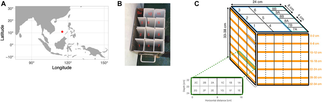
FIGURE 2. Location and setup of the boxcore OR1-1218-C2-BC. (A) Sampling location of the boxcore in the South China Sea. (B) Photo of the setup and the plastic tubes (courtesy of Yu-Huang Chen), the sub-cores 11 and 12 are not analyzed. (C) Schematic overview of the individual samples analyzed from the boxcore. Within each sub-core, seven depth layers were sampled for radiocarbon analyses (orange layers): 0–2, 6–8, 10–12, 16–18, 22–24, 28–30 and 32–34 cm. A detailed overview of the sample sizes is given in Table 1. Sub-core 1 was further used for small sample analyses (gray excerpt), and together with sub-core 2 for small-volume bulk sample measurements (22–23 and 23–24 cm, green excerpt).

We use the radiocarbon content in foraminiferal tests as a proxy of time since deposition. Following the different intensity and spatial extent of mixing and burrowing activities, the vertical and horizontal heterogeneity, which is a result of reworking by e.g. bottom currents and the displacement of foraminifera shells by benthic fauna (Figure 1B), might vary on different spatial dimensions from millimeters to decimeters. To guide our sampling strategy and interpretation, we posit that the overall age-heterogeneity can be described by the two terms defined below and illustrated in the idealized sketch of a two-dimensional sediment slice (Figure 1C).

1) The term mixing is used here as a description of the heterogeneity within a sample, i.e. the variations between individual specimens in a finite volume, which is the result of the uniform mixing over a certain depth interval. This in-sample heterogeneity can be overcome by measuring a large number of specimens.

2) The horizontal heterogeneity in the mean age can be thought of as a net displacement of the sediment. It describes the deviation of a sample from the mean age-depth relationship. In addition to the process of mixing, this is also dependent on the sediment accumulation rate and the presence of trace fossils and resulting post-depositional modifications.

2.2 Core Setup and Sampling

The sediment core OR1-1218-C2-BC was taken in March 2019 onboard the research vessel Ocean Researcher 1 (OR1). The sediment consists of beige and light brown silty foraminiferal ooze. The core was directly divided into twelve sub-cores onboard the ship by pushing plastic tubes into the sediment (Figure 2B). Here, the sub-cores OR1-1218-C2-BC-1 to 9 (in the following we only refer to sub-cores 1–9) were analyzed. The oxygen content of the core was not measured, but the number of fossil traces indicates oxygen-rich conditions (Savrda, 2007). The subsequent sampling was performed in the PaleoProxy Lab at the Institute of Oceanography, National Taiwan University, Taipei, Taiwan. From each sub-core, a thin slab with 1 cm thickness along the length of the core was taken for X-ray radiography before the sub-cores were split into smaller samples. The sub-cores 1 to 5 were vertically sampled in 2 cm thick slices and the sub-cores 6 to 9 in 1 cm slices. The sub-cores 7 to 9 were additionally horizontally split into two parts, A and B (Figure 2C). All samples were freeze-dried, wet-sieved through a 63 μm mesh and dried at 50 °C before foraminiferal tests were picked. All analyses were based on the most abundant planktonic foraminiferal species Trilobatus sacculifer (T. sacculifer, without sac-like final chamber, 315–355 μm size fraction).

The sub-cores extracted from the box core were of different lengths, ranging between 33.5 and 38 cm (Table 1). We restricted the measurements to a maximum depth of 34 cm for all but sub-core 1, on which the first ¹⁴C measurements were performed with 130 and 165 specimens for the depths from 0 to 1 and 36–37 cm, respectively, to estimate the age range covered by the core. Additionally, three replicates with 200 specimens from the depth of 36–37 cm from sub-core 1 were measured for a preliminary estimate of the sediment mixing intensity.

TABLE 1

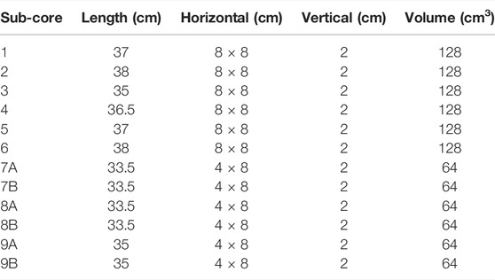
TABLE 1. Overview of different parameters from the sub-cores 1 to 9: lengths of the individual sub-cores, the measured horizontal and vertical sample size and the resulting volume for each large-volume bulk sample.

The sampling was divided into three types with the aim to investigate the afore-described processes which cause age-heterogeneity between individual specimens as well as among samples. The types differ in terms of the number of picked and measured specimens as well as the volume of the samples:

• Large-volume bulk samples. The age of the seven depth layers from each of the twelve sub-cores (indicated in orange in Figure 2C) was determined with samples based on volumes of 128 cm³ (=  2 × 8 × 8 cm) for the sub-cores 1 to 6 and 64 cm³ (=  2 × 4 × 8 cm) for the sub-cores 7A to 9B (Table 1). From each sample, 200 foraminiferal tests were picked, gently crushed and well mixed, so that each aliquot of the sample would contain material from a large proportion of the individuals, and thus would reflect the mean age of the sample. The crushing and mixing is important as only about one-third of each sample ( ∼800 μg CaCO₃) was used for each ¹⁴C measurement in order to have remaining material for either a replicate measurement or a measurement of another proxy from the same batch of individuals (e.g. δ¹⁸O). These age estimates based on large-volume bulk samples are used to quantify spatial patterns of net vertical displacement of sediment leading to horizontal variation in the mean age.

• Small-volume bulk samples. From sub-core 1 and 2, small-volume samples with a volume of 1.8 cm³ (= 1 × 1.8 × 1 cm) were taken from thin slabs for two depth layers (22–23 and 23–24 cm, indicated in green in Figure 2C zoom-in). As for the large-volume bulk samples, 200 specimens were picked, crushed and about one third of each sample (∼800 μg CaCO3) was used for radiocarbon measurements. These data are used to test whether the net displacement depends on the spatial scale and thus the sample volume.

• Small-n samples. Ten replicates of five specimens were measured for the depth layers 6–8 and 36–37 cm from sub-core 1 (indicated in gray in Figure 2C zoom-in). In contrast to the 200 foraminifera samples, which are intended to average out the variation between individuals in a sample so that differences between distinct sediment volumes can be measured, these small-n samples are used to determine the within-sample age-heterogeneity and the vertical extent of the mixing. Samples from two different depths were used to test whether the mixing changed along the core and over time. However, the upper depth might be less reliable because it lies within the actively mixed layer.

All measurements were performed with an accelerator mass spectrometer Mini Carbon Dating System (MICADAS) equipt with a Carbonate Handling System (CHS) and Gas Interface System (GIS) at the Alfred Wegener Institute in Bremerhaven, Germany (Wacker et al., 2010; Mollenhauer et al., 2021). All samples were prepared and measured as gas targets following the standard operating procedures described by Mollenhauer et al. (2021). Briefly, all samples were weighed into 4.5 mL septum sealed vials, loaded into the CHS and flushed with ultra-pure helium for 5 min with 70 mL min⁻¹ to remove all traces of atmospheric CO₂ using a two-way needle. After addition of 200 μL phosphoric acid (H₃PO₄, ⩾85%, Fluka 30,417) the hydrolyzation reaction took place over ∼30 min at 70 °C. Following complete hydrolysis, sample CO₂ was flushed from the vial for 1 min at 70 mL min⁻¹ He flow and passed over a phosphorus pentoxide trap to remove water vapor. CO₂ was subsequently concentrated on the zeolith trap of the GIS, quantified manometrically and fed into the ion source. Radiocarbon data were normalized against standard gas (CO₂ produced from NIST Oxalic Acid II, NIST SRM4990C) and blank corrected against sample size-matched blank foraminifera (pre-Eemian age) processed alongside the samples (Mollenhauer et al., 2021).

All radiocarbon data were calibrated and converted to calendar ages based on the Marine20 calibration (Heaton et al., 2020) using the R package Bchron (Haslett and Parnell, 2008; R version 4.0.3; R Core Team, 2020). We used the default reservoir age provided in Marine20 and did not adjust for local marine reservoir effects because we are only comparing relative, and not absolute ages.

Besides the processes affecting the signal prior to the core extraction, a number of steps during the sampling can also result in biases. A tilted incline of the corer at the seabed can result in skewed layers within the core and can lead to differences in derived parameters from different sides of the core especially when compared by sediment depth. Additional biases can arise from an imprecise manual sampling of single layers and from the preferential preservation of younger specimens due to their shorter residence time in the sediment compared to older counterparts. We carefully examined our data set with respect to the described errors by analyzing the difference in age between different sides of the core. We did not find any indication for biases in the core retrieval, the manual sampling or the preferential preservation of younger specimens.

2.3 Estimation of the Sediment Accumulation Rate

The sediment accumulation rate is derived from a simulation with the depth-age model BACON (Blaauw and Christen, 2011) using a vertical resolution of 1 cm and the Marine20 calibration curve (Heaton et al., 2020) to convert raw ¹⁴C data to calendar ages. We use all radiocarbon data for this approach, with the small-volume bulk samples and the small-n samples averaged for their respective depths.

2.4 Estimation of the Sediment Mixing Strength

The variation in age between individual foraminifera from the same depth, σ_ind, can be used as a measure of the sediment mixing strength. As our current analytical capabilities do not allow us to measure the radiocarbon content of a single T. sacculifer test, we instead measure ¹⁴C on samples of 5 individuals, and rescale the variance between them following Dolman et al. (2021a). To obtain σ_ind from σ_rep we first subtract the measurement error variance, σ_meas, before multiplying by the number of individual specimens, n_f, and taking the square root. σ_meas includes the reported measurement error and the additional uncertainty from the calibration to calendar age.

${\sigma }_{\mathit{ind}}=\sqrt{n_f\left({\sigma }_{\mathit{rep}}^2-{\sigma }_{\mathit{meas}}^2\right)}(1)$

If σ_ind is rescaled using the sediment accumulation rate, it represents the average distance that individual particles have been moved by mixing, and in a simple 1-box mixing model, it can be thought of as the mixing depth (e.g. Berger and Heath, 1968).

2.5 Estimation of the Net Sediment Displacement

The variations in derived ¹⁴C ages from the small- and large-volume bulk samples are used to describe the net sediment displacement, i.e. the effect of the spatially non-uniform mixing on the mean age of a sample. We evaluate this by analyzing the deviations of the individual age estimates to the respective mean of each depth layer corrected for the expected variations due to the large but still finite sample size. To only study the effect of the net displacement, we subtract the variations caused by the measurement error and the calibration as well as from the finite sample size.

2.6 Visual Assessment of Mixing

Radiograph images were taken from the thin slabs at the Institute of Oceanography at the National Taiwan University, Taipei, Taiwan, and are, together with optical photographs, used to qualitatively determine the mixing extent and intensity. Both types of images allow a visual inspection of the mixing conditions and a separation between homogeneously mixed material with a mottled appearance and the historical layer with potential deep reaching burrows (e.g. Löwemark and Werner, 2001; Löwemark, 2015).

3 Results

In the following, we present the results of the individual ¹⁴C measurements, grouped by sampling approach as described in Section 2.2. We then derive the sediment accumulation rate (Section 3.2) as well as the extent (Section 3.3) and the spatial structure of the mixing (Section 3.4) before describing different error terms affecting the reliability of derived age estimates (Section 3.5).

3.1 Radiocarbon Measurements

3.1.1 Large-Volume Bulk Samples

The youngest calibrated ¹⁴C age estimate from the large-volume bulk samples is 1,803 years (±109 years 1 standard deviation (SD) measurement error), while the oldest sample has an age of 18,333 years (±226 years). The horizontal standard deviations (σ_cores) in each depth layer vary between 471 (22–24 cm) and 1,354 years (32–34 cm). Generally, the range of ages, the standard deviations within a depth layer and the measurement errors (σ_meas) increase with sediment depth and age (Figure 3; Table 2).

FIGURE 3

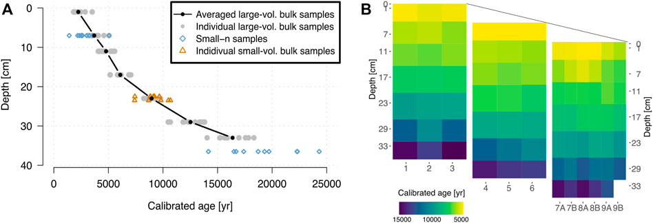
FIGURE 3. Depth-age illustrations for calibrated radiocarbon ages. (A) Calibrated ages for the large-volume bulk samples are shown with gray points and their respective mean per depth layer illustrated in black. Measurement errors for single data points are not displayed due to their small magnitude. The blue diamonds are age estimates based on small-n samples while the golden triangles show ages from the small-volume bulk samples. (B) Absolute calibrated calendar ages from the large-volume bulk samples are illustrated for each sub-core and arranged according to the sub-sampling of the core to illustrate the three dimensions (see Figure 2B).

TABLE 2

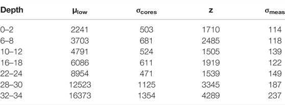
TABLE 2. Overview of calibrated calendar ages derived from the¹⁴C measurements of the low-resolution bulk samples. For each depth interval (in cm), the mean age (μ_lowres), the standard deviation (σ_cores), the total range (z = max_age − min_age) as well as the mean measurement error (σ_meas) of all twelve subcores (see Table 1) are given in years. For the layer from 32 to 34 cm, the data point from sub-core 9B had to be removed due to reported problems during the measurement and is not included in the analyses.

3.1.2 Small-Volume Bulk Samples

To investigate whether and how the net displacement varies in space, we analyzed the horizontal variations in the small-volume bulk samples (1.8 cm³). The mean ages of the small-volume samples are similar to those of the large-volume bulk samples from their respective depth and sub-core, and agree within the standard error. However, the small-volume samples show a significantly higher variance than the large-volume samples (golden triangles vs. gray points, Figure 3A, F-test with p = 0.01) with a SD of 1,089 years for the small-volume samples compared to 471 years for the large-volume samples, despite being based on measurements with the same number of foraminiferal tests.

3.1.3 Small-n Samples and Age Heterogeneity

To infer the age-heterogeneity within a sediment sample and thus the mixing, the replicated measurements of the small-n samples from 6 to 8 and 36–37 cm from sub-core 1 are used. The mean age for the upper layer is 2,849 years with σ_rep of 977 years, and 19,140 years with a SD of 3,126 years for the deeper layer (Table 3, individual data points in Figure 3A). The inferred SD between single foraminifera, σ_ind (Eq. 1), which can be seen as an estimate for the heterogeneity in ages within a sample, is 2,184 years for the upper layer and 6,990 years for the deeper layer. The mean of the small-n samples from 6 to 8 cm is younger than the large-volume samples mean (2,849 vs. 3,703 years, Table 2), but this difference is not statistically significant.

TABLE 3

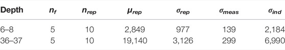
TABLE 3. Replicated¹⁴C measurements on small-n samples from sub-core 1. The number of measured specimens n_f as well as the number of replicate measurements n_rep is given. μ_rep is the mean of replicated age estimates per depth layer, σ_rep the standard deviation and σ_meas the mean measurement error. σ_ind is the inferred standard deviation in age between individual samples, following Dolman et al. (2021a). All estimates are given in years.

3.2 Sediment Accumulation Rate

With an average age of 2,241 years for the top layer and 19,140 years for the lowest measured layer (36–37 cm), the sediment core covers the Holocene and the last glacial termination. The sediment accumulation rate was determined using the BACON model (Blaauw and Christen, 2011). To obtain estimates at a spatial scale comparable to the extent of mixing, we applied a running mean with a width of 10 cm to the derived accumulation rate model. For the upper part of the core (10–18 cm, disregarding the mixed layer), the model suggests an average sediment accumulation rate of 3.4 cm kyr⁻¹ (Figure 4) while the deeper part of the core is characterized by a transition to lower sediment accumulation rates with a mean of 1.6 cm kyr⁻¹ (>18 cm).

FIGURE 4

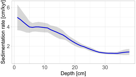
FIGURE 4. Derived sediment accumulation rates using the BACON model and all ¹⁴C ages (averages of the small-volume bulk and the small-n samples). The rate decreases from the upper core part towards the bottom of the core. The confidence intervals are ± one standard deviation of all realizations from BACON.

3.3 Sediment Mixing and Bioturbation Depth Estimates

Visual analyses of optical images and radiographs are used to distinguish between a homogeneously mixed layer at the top of each sub-core, followed by increasingly distinct burrows which mark the transition to the historical layer with single deep reaching burrows, such as Zoophycos (Figure 5). The exemplarily shown sub-core 2 illustrates the vertical extent of sediment mixing which can be described with a homogeneous color in the photograph and a mottled appearance in the radiograph. The homogeneously mixed layer extends to about 8 cm, followed by the transition from the increasingly distinct burrows to the historical layer between 12 and 13 cm. The historical layer is characterized by lighter and darker colors in the image, the occurrence of individual deep reaching burrows (Figure 5, marked in red) and loosely filled burrows (orange marks).

FIGURE 5

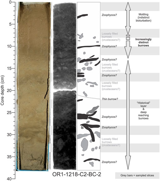
FIGURE 5. Assessment of the vertical extent of sediment mixing as well as the intensity by visually analyzing photograph and radiograph images from sub-core 2 exemplarily. All images are in the Supplementary Figure S1. The radiograph image was done on a thin slab (∼1 cm thick sediment slice). Possible burrowing activities are indicated on the radiograph image for Zoophycos (black) and loosely filled burrows (gray). The characteristic depth intervals of bioturbated sediments are described as well. Horizontal gray bars indicate the sampled layers for ¹⁴C analyses.

Similar structures are also found in all other cores (Supplementary Figure S1). The average extent of the mixed layer is 8.4 ± 1.2 cm (1 SD) and the transition to the historical layer occurs on average at 12.8 ± 0.9 cm. The visual assessment indicates horizontal variability for all analyzed layers within the core. Individual depths for each sub-core are listed in the Supplementary Table S1.

In addition to the visual inspection of images, we used the derived age-heterogeneity from the small-n data together with the sediment accumulation rate (Section 3.2) to derive a mixing depth. Depending on the considered depth interval and the accumulation rate, we derive a bioturbation depth between 7.5 and 11 cm, consistent with the independent visual estimates.

3.4 Spatial Structure of Sediment Mixing

The individual age-depth profiles in Figure 3 indicate a continuous increase of age with depth for each sub-core. However, the horizontal structure shows spatial variability within single depth layers (Figure 6). Variations within a depth layer increase with depth, exceeding ± 2,000 years with large standard deviations for depths from 28 to 30 cm and 32–34 cm (Table 2). The resulting heterogeneous spatial variability in the large-volume three-dimensional residuals (Figure 6) indicates spatial coherence: the right panel for the sub-cores 7A to 9B is often younger than its neighboring panel for the sub-cores 4 to 6. Notably, the sub-cores 7A and 9B show consistently younger ages while sub-core 5 is consistently older than the average age. These patterns were tested for spatial autocorrelation with a 3D Moran’s I (Moran, 1950) and are statistically significant (p < 0.05) which indicates more spatial clustering than expected from a random process.

FIGURE 6

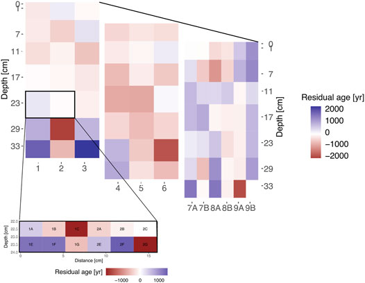
FIGURE 6. Three-dimensional view on age-heterogeneity within the core. Residuals to the respective mean of each depth layer are shown for all twelve sub-cores. They generally increase with depth and show the largest deviations towards the bottom of the core. Residuals from the small-volume bulk samples are compared to the overall mean of all twelve samples and are shown in the insert.

The horizontal variability derived from the small-volume bulk samples (zoom-in panel in Figure 6) suggests that the spatial scale of mixing is smaller than the volume of the large samples which implies a dependency on the spatial scale of measurements.

3.5 Components of Age Uncertainty

Uncertainties in age-depth profiles are usually based on analytical error terms, specifically the measurement error which is reported by the laboratory and its conversion to calendar ages. However, additional uncertainties arise from both picking a finite number of specimens from a mixed sediment sample, and from horizontal variation in mean age. In order to account for these uncertainties, we assess the error terms from the measurement and calibration process, from the finite number of specimens as well as from the net displacement of sediment material (Figure 7). The first error term is the calibrated value of the reported uncertainty (derived from ¹⁴C counting statistic) from the MICADAS laboratory and increases with depth due to the exponential decay of radiocarbon (mean of 152 years, individual estimates per depth layer are in Table 4). The error from picking and measuring a finite number of specimens can be expressed by σ_ind from the small-n samples divided by the square root of the number of picked specimens. This term shows a mean uncertainty of 325 years and increases with depth due to the decreasing sediment accumulation rate. We use this term as an approximation of the expected heterogeneity within the bulk-samples based on the derived age-heterogeneity in the small-n samples from 6 to 8 and 36–37 cm. The spatial age-heterogeneity σ_cores is the standard deviation of all large-volume bulk ¹⁴C ages for each depth layer respectively. Due to the change in sediment accumulation rate with depth, the age uncertainty increases with depth from 291 to 1,253 years (mean 673 years) while the net vertical displacement in depth stays between 0.6 and 2.6 cm (mean 1.7 cm).

FIGURE 7

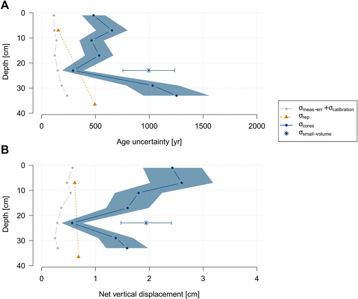
FIGURE 7. Different error terms affecting the reliability of ¹⁴C ages derived from large-volume bulk (200 foraminifera) samples. The measurement error (σ_meas−err) is shown combined with the uncertainty from the calendar age calibration (σ_calibration, gray). Sampling only a finite number of specimens (σ_rep, orange) leads to an additional uncertainty term which increases with decreasing sediment accumulation rates. The largest contribution to the overall uncertainty stems from the horizontal age-heterogeneity which is represented as the standard deviation per depth layer between the large-volume bulk samples from all sub-cores (σ_cores, blue). The small-volume bulk samples (σ_{small−volume}, blue star) show an even larger uncertainty due to the smaller physical volume. The variations caused by the measurement error and the finite sample size are subtracted from both σ_cores and σ_{small−volume} to show the true effect of the net displacement. The error terms are illustrated for (A) resulting age uncertainty and (B) the net vertical displacement by considering the change in sediment accumulation rate with depth (Figure 4). The confidence interval and the error bar are the standard deviation of the standard deviation of the bulk samples, but in (B) not accounting for the uncertainty in the sediment accumulation rate.

TABLE 4

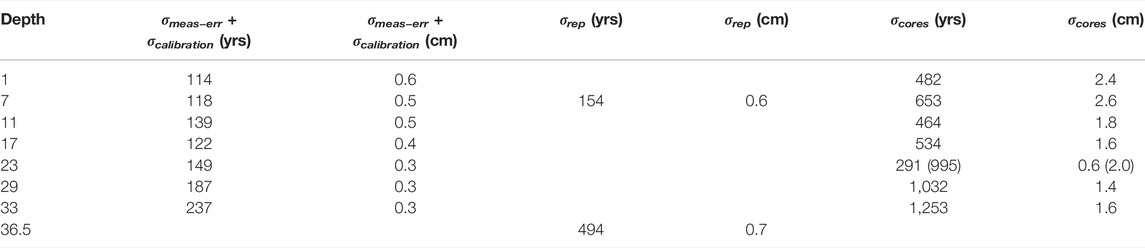
TABLE 4. Contributions to age and depth uncertainty from different error terms. The error terms are described and illustrated in Section 3.5. The error from the standard deviation across all large-volume bulk samples (σ_cores) is the remaining uncertainty after accounting for σ_meas−err, σ_calibration and an interpolated estimate of σ_rep. For the small-volume bulk samples, σ_{small−volume} is mentioned in brackets at 23 cm depth. The depth estimates are derived by scaling the age estimates with the sediment accumulation rate output from the BACON model.

4 Discussion

If sedimentation and mixing within the sediment is spatially uniform, neighboring cores would be affected in the same way and thus, nearby records should demonstrate replicable profiles. In contrast, if mixing is incomplete, patchy or heterogeneous, the afore-mentioned simple assumption does not hold and proxy records from nearby cores will display differences due to their unique mixing history.

Following the simple assumption of a homogeneous mixed layer (Figure 1A), the transition to the historical layer is characterized by a kink in the depth-age-relation and this depth is interpreted as the mixing depth (Berger and Heath, 1968; Berger and Killingley, 1982; Trauth et al., 1997). This might be true if the mixing is intense and sediment accumulation rate low. However, even though both of these apply to the core shown here, we do not find a distinct kink in the ¹⁴C record which suggests that mixing is incomplete, or spatially and temporally variable mixing describes the conditions more realistically (Figure 1B).

From previous studies, we recognise the importance of sediment mixing for proxy records and its influence on the representativity of such reconstructions. The mixing leads to additional uncertainty in the determination of the samples’ age (e.g. Barker et al., 2007; Díaz-Asencio et al., 2020; Lougheed et al., 2020; Dolman et al., 2021a) and to a smoothing of the signal (Anderson, 2001). We can use simple models to estimate the additional noise as well as the magnitude of smoothing. However, these models assume homogeneous mixing which underestimates the afore-described spatial variability. Besides the active mixing, age-heterogeneity and age offsets can also arise from changes in the foraminiferal flux (i.e. the number of specimens per cubic centimeter) which can amplify or reduce the variations caused by mixing. Changes in the flux are driven by variations in the surface productivity and/or the thermal structure of the upper water column (Bard et al., 1987; Jian et al., 2000); thus, also containing environmental information. However, the abundance of T. sacculifer does not change along our sediment core and is consequently not the factor causing the age-heterogeneity.

Likewise, selective bioturbation of different size-fractions can result in biased age estimates (Peng et al., 1979; Broecker et al., 1984). Our study is based on the size fraction from 315 to 355 μm, thus our results might be invalid for the fine material and other size fractions which are differently affected by mixing (Wheatcroft, 1992; Díaz-Asencio et al., 2020). In addition, changing corrosivity of bottom water mass over time, oxygen-related changes in the benthic faunal community or preferential dissolution of older foraminifera shells due to their relatively longer residence time in the sediment can bias age estimates (Barker et al., 2007). However, we expect that dissolution at our study site is not important because the water depth at the core location lies above the typical depth of the lysocline in the South China Sea where the water is saturated with calcium carbonate (e.g. Regenberg et al., 2014; Wang et al., 2016). We also find no trend toward lower diversity in trace fossils or a change in sediment color from brown to gray, both of which would indicate changes in oxygen levels (e.g. Froelich et al., 1979; Savrda, 2007). We therefore interpret our observations as variability caused by mixing and discuss its spatial scale in the following.

4.1 The Spatial Scale of Mixing and Sediment Heterogeneity

The conventionally considered error terms of the measurement and the calibration process underestimate the true uncertainty of the age-depth relationship that includes also spatial displacement (Figure 7), and disregard deep reaching bioturbation effects, e.g. the formation of spreiten, which can lead to significant deviations from the mean age and severe offsets in the horizontal age structure (Löwemark and Werner, 2001; Leuschner et al., 2002; Löwemark and Grootes, 2004). The magnitude of different error terms (Section 3.5) is dependent on the sediment accumulation rate and can therefore be different in age and depth units.

Figures 8A,B illustrate in three dimensions the scale and pattern of variation in age that could be generated from the independent ¹⁴C measurement error and the measurement of a finite number of specimens from a homogeneously mixed sediment, respectively. Figure 8C shows the pattern observed in the real data, which differs from that shown in the previous two figures, suggesting that it likely contains a component of incomplete and/or heterogeneous mixing leading to net displacement. The assumption that mixing is at least partly responsible for the clustering of spatial patterns from e.g. burrowing activities and resulting low reproducibility of nearby cores can be confirmed with a statistically significant spatial correlation within the presented core (Moran’s I, p < 0.05).

FIGURE 8

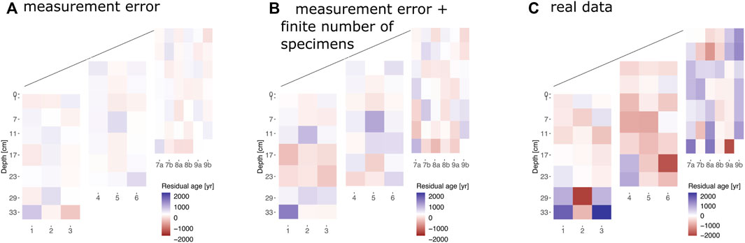
FIGURE 8. An illustration of the effect of different error terms on the three-dimensional variability of ¹⁴C derived age estimates. The deviations from the mean age per depth layer are smallest considering (A) only a random measurement error (including the calendar age calibration error) and increase when (B) the finite number of randomly picked and measured specimens is taken into account. (C) The horizontal age-heterogeneity derived from all sub-cores (Figure 7, σ_cores) exceeds both deviations and shows the true age-heterogeneity caused by mixing.

The presented variability in Figure 8C is based on the large-volume bulk samples (200 specimens from volumes of 64 or 128 cm³) which averages out small structures within the sediment, whereas age estimates from small-volume samples with 1.8 cm³ are more likely to be influenced by small-scale mixing structures, have larger standard deviations and are less indicative for the mean age of a depth layer (Figures 3,6). As most proxy analyses are performed on sample volumes of 10–20 cm³, the applicable net displacement and its uncertainties would be in between our estimates from the small- and large-volume samples and are likely contained but potentially not considered in conventional proxy analysis. Using fewer specimens increases the range of age estimates for a given depth layer which would rather be indicative of short-term local ¹⁴C changes, such as upwelling and monsoonal activities for our study site in the South China Sea (e.g. Xie et al., 2003; Tan et al., 2020), instead of the true mean age of the layer which is desired for reliable age-depth modeling.

The question remains to what extent our findings apply to other sediment sites used for paleo-reconstructions. In most cases, age-models are not replicated. In the replicated down-core radiocarbon age estimates from different tubes from a multicore (SO213-84-2, Figure 7 in Dolman et al., 2021a), the difference between age models is one order of magnitude higher than expected from the uncertainty from the radiocarbon measurements which provides strong evidence for a significant net displacement. Furthermore, an indirect evidence for sediment mixing can be found in age-model reversals as seen in larger compilations of marine proxy records which regularly contain age-reversals in their chronologies (38% of the age-models in the marine compilation in Marcott et al., 2013 contain an age reversal, 19% have a reversal larger than twice the given uncertainty bounds). The true number might be even higher because cores or core-sections with difficult age-models may sometimes remain unpublished even though this might simply be the result of active sediment mixing. Thus, our findings are likely applicable beyond our study site but similar studies at other sites would be very useful to investigate the dependence of the sedimentation setting.

The magnitude of the errors associated with a¹⁴C age estimate influences the shape of a potential depth-age relationship. An example of a BACON realization for sub-core 8B (vertical resolution of 1 cm) with conventional error estimates based only on the uncertainty stemming from the measurement and calibration (as in Figure 8A) shows that most of the age estimates from the other sub-cores lie outside of the suggested 95% confidence interval (Supplementary Figure S2A). In contrast, when the observed variability in age estimates (Figure 8C) is used as an error estimate, the BACON model (not surprisingly) shows an overlap of the confidence intervals with most of the individual age estimates (Supplementary Figure S2B). Hence, it may be useful to include the effect of the net displacement, i.e. that a dated sample might not represent the correct age for the layer it was sampled from, into age-model strategies for marine sediments. A similar strategy was proposed for lake sediments already (Heegaard et al., 2005).

4.2 Potential Implications for Paleo-Reconstructions

While the classical uncertainty of radiocarbon dates (derived from ¹⁴C counting statistic, σ_meas−err + σ_calibration) is independent of the sedimentation rate, the effect of measuring radiocarbon dates on a finite number of foraminifera in a mixed sediment (σ_rep) and the effect of the net displacement (σ_cores) are inversely proportional to the sedimentation rate and thus most important for low sedimentation conditions. For example, assuming a 10 cm sedimentation rate; a net displacement of 2 cm would lead to an additional 200 years (1 SD) uncertainty from the net displacement comparable to the typical radiocarbon uncertainty in the Holocene.

While for single records, such an age uncertainty might not affect the inferred conclusions, it does, however, affect the comparison between records from different sites, between reconstructed climate and independent forcing time-series as well as large scale stacks of records. For example, Marcott et al. (2013) (their SI Figure 17) estimated that in the global mean Holocene stack, variability at millennial scales (1/1000 years) is underestimated by a factor of two, mainly caused by the radiocarbon age-uncertainty. If we speculate that the true time uncertainty is 30% times larger due to mixing and net displacement as shown here, this would imply that millennial scale variations might be damped by a factor of five in the reconstructions. Thus, the smooth reconstructed Holocene temperature evolution might be further away from the true temperature variations. Reschke et al. (2019b) used the correlation between nearby records to estimate the signal to noise ratio in marine sediment records. The study found that the results were strongly dependent on the age uncertainty estimates; if the true age uncertainty is considerably stronger than usually assumed, as proposed here, this would also imply that the signal to noise ratio and thus the quality of the sediment records is higher than suggested by Reschke et al. (2019b). Given the importance of knowing the accurate age-uncertainty, estimates of the mixing and the net displacement for other sedimentation conditions would be very valuable for quantitative paleo-reconstructions.

4.3 Suggested ¹⁴C Measurement Strategy to Determine Mixing and Net Displacement and to Enable a Reliable Dating

A number of studies already compared different dating strategies (e.g. Andree, 1987; Blaauw et al., 2018; Lacourse and Gajewski, 2020) and we therefore do not want to propose an all-encompassing strategy, as this also depends on external conditions, such as financial and laboratory capacity, as well as the individual characteristics of each core. For studies which need reliable dating with a precise quantification of the age-model uncertainty and mixing, we suggest a sampling strategy based on our findings (Figure 9). It should be noted, however, that our suggestions focus on sampling strategies for optimal age modeling to derive from this information on the uncertainty inherent in the reconstructed proxy data that should be considered in the interpretation. Moreover, these results and recommendations apply to bioturbated sediments and would not apply to sediment cores which are clearly laminated or show other signs that they were deposited in dysoxic or anoxic conditions.

FIGURE 9

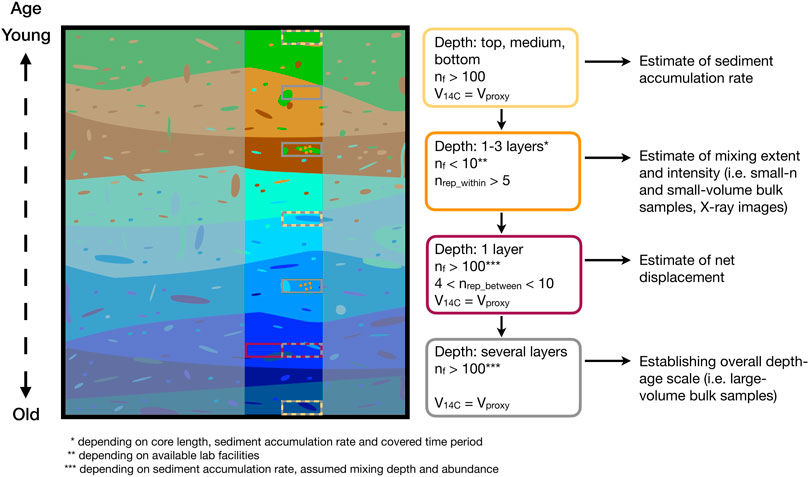
FIGURE 9. Overview and illustration suggested steps towards an improved sampling protocol for a single core. The boxes correspond to proposed samples in the 2D sketch and contain suggestions for different sample types with the depth and the number of layers to samples, the ideal number of specimens n_f, the number of replicates n_rep−within from one sample or the number of replicated samples from one depth n_{rep−between} as well as the physical volume of a sample V_14C. The sample volume should be similar or the same as the volume used for the proxy reconstruction (i.e. 10 - 20 cm³). The second row indicates the information which can be derived from each individual sample type and it indicates to which of the samples from our study it can be compared.

We recommend sampling in batches to adapt it to the accumulation characteristics of the core. Specific suggestions on the replications, the number of specimens and the sample volumes are mentioned in Figure 9. Samples for the age determination should have a similar sediment volume as those for the proxy, so that they are affected by the same sediment heterogeneity. Furthermore, if proxy and radiocarbon measurements are based on the same sedimentary material, e.g. calcite tests, they should be derived from the same sediment sample instead of two smaller sediment samples from the same depth. The minimal number of shells to measure in order to derive reliable age estimates can be approximated with the information on the sediment accumulation rate and the mixing depth as well as with calculations and reference charts (e.g. Eq. 5 and Figure 8 in Dolman et al., 2021a).

The ultimate aim of each dating approach is to establish a reliable depth-age scale. A first approximation of the covered temporal period of a core and a rough estimate of the sediment accumulation rate can be derived with age estimates ideally based on a large number of specimens from the top and the bottom of a core. An additional data point at an intermediate depth can provide information on the consistency of the sediment accumulation rate.

Replicated measurements of small numbers of foraminifera (10 × 5 specimens) from the same sample can be sampled from several depths to infer the mixing extent and intensity. Similar approaches were applied in previous studies and provided reliable estimates (e.g. Lougheed et al., 2018; Fagault et al., 2019; Dolman et al., 2021a). Additional information on the presence of bioturbational structures from trace fossils and their intensity (e.g. Zoophycos, Figure 5 and Supplementary Figure S1) can be obtained from X-ray images. To further assess the small-scale heterogeneity among samples, we recommend the sampling of several horizontal samples, if possible. This might be restricted by the available core diameter and material, but will provide valuable insights.

As a last step, measurements with many specimens from large volumes for multiple, regularly spaced intervals can be performed. A high vertical density is desired but depends on the sedimentary conditions and might be limited by the availability of material and the financial resources. However, applying the strategy on a limited number of cores in different sedimentation conditions would allow an estimation the range of expected age displacements and thus allow for more realistic age-depth models including uncertainty estimates in the future.

5 Conclusion

The analysis of radiocarbon in foraminiferal tests as a tracer of time since deposition shows at a first sight that all sub-cores showed an agreement on the temporal ¹⁴C decrease from the early Holocene to the last glacial termination. However, the detailed investigation of the three-dimensional variability in ages pointed out a much larger uncertainty than what is usually accounted for in depth-age models. This is to some extent caused by the measurement of a finite number of specimens which leads to an uncertain estimate of the true age. An additional contribution to the increased uncertainty is the (vertical) displacement of sedimentary material which is more pronounced in small volume samples. Even if all of these parameters were taken into account, there is a lack of clear delineation or kink in the ¹⁴C record between the mixed and the historical layer, which is often used in studies or simulations as a determination of the bioturbation depth (e.g. Berger and Heath, 1968; Berger and Killingley, 1982).

The new estimation of uncertainties implies that the traditionally considered errors related to ¹⁴C derived ages are likely too optimistic. Both the mixing and the sediment displacement affect the representativity of a derived age estimate in a way which is not clearly quantified yet. We provide a data-based estimate of the vertical net displacement indicating that the depth of a specific age might vary by up to 3 cm from one core to another with an effective age uncertainty about five times larger than usually assumed. If resources and funding permit, we recommend replicated radiocarbon measurements of samples with small numbers of foraminifera, e.g. 10 × 5 specimens for one or two depths, and (replicated) measurements based on many specimens of large-volume samples, e.g. core halves, to quantify the full magnitude of uncertainty for the age-depth model. An examination of the spatial variability of age estimates under other sedimentary conditions, e.g. higher sediment accumulation rates or weaker/stronger mixing, would allow a more detailed description of the effects and a parameterisation of these in depth-age models.

Data Availability Statement

The datasets presented in this study can be found in online repositories. The names of the repository/repositories and accession number(s) can be found below: Radiocarbon data and associated calibrated age information are submitted to the PANGAEA repository. AZ, AD, SH, JG, HG, C-CS, TL (2022): Radiocarbon age measurements on foraminifera from sediment core OR1-1218-C2-BC. PANGAEA, https://doi.pangaea.de/10.1594/PANGAEA.942239.

Author Contributions

TL, SH and AZ designed the study. C-CS performed the fieldwork with the help of the crew of the research vessel OR1. AZ and SH did the subsampling at the Institute of Oceanography, Taiwan, and JG and HG carried out the picking of specimens and measuring of samples. LL performed the X-ray measurements and the analysis of the X-ray radiograph images. AZ performed the statistical analysis with help from AD and TL. All co-authors contributed with their specific expertise to the interpretation of the data. AZ prepared the manuscript with contributions from all co-authors.

Funding

This is a contribution to the SPACE ERC project; this project has received funding from the European Research Council (ERC) under the European Union’s Horizon 2020 research and innovation program (Grant Agreement No: 716092). Additionally, this work was supported by the German Federal Ministry of Education and Research (BMBF) as Research for Sustainability initiative (FONA); www.fona.de through the Palmod project (FKZ: 01LP1509C). SH and LL acknowledge support from the Taiwanese Ministry of Science and Technology (Grant Number 107-2611-M-002–021-MY3 and 108–2116-M-002–007, respectively).

Conflict of Interest

The authors declare that the research was conducted in the absence of any commercial or financial relationships that could be construed as a potential conflict of interest.

Publisher’s Note

All claims expressed in this article are solely those of the authors and do not necessarily represent those of their affiliated organizations, or those of the publisher, the editors and the reviewers. Any product that may be evaluated in this article, or claim that may be made by its manufacturer, is not guaranteed or endorsed by the publisher.

Acknowledgments

We thank the scientists and the crew of the OR1-1218 expedition on board the research vessel Ocean Researcher 1 who helped with sample retrieval. We also thank Akshat Gopalakrishnan, Lena Kafemann and Tina Palme for picking the foraminifera and the AWI MICADAS team for carrying out the radiocarbon measurements.

Supplementary Material

The Supplementary Material for this article can be found online at: https://www.frontiersin.org/articles/10.3389/feart.2022.871902/full#supplementary-material

References

Anderson, D. M. (2001). Attenuation of Millennial-Scale Events by Bioturbation in Marine Sediments. Paleoceanography 16, 352–357. doi:10.1029/2000PA000530

CrossRef Full Text | Google Scholar

Andree, M. (1987). The Impact of Bioturbation on AMS 14C Dates on Handpicked Foraminifera: A Statistical Model. Radiocarbon 29, 169–175. doi:10.1017/S0033822200056927

CrossRef Full Text | Google Scholar

Bard, E., Arnold, M., Duprat, J., Moyes, J., and Duplessy, J.-C. (1987). Reconstruction of the Last Deglaciation: Deconvolved Records of ?18O Profiles, Micropaleontological Variations and Accelerator Mass spectrometric14C Dating. Clim. Dyn. 1, 101–112. doi:10.1007/BF01054479

CrossRef Full Text | Google Scholar

Bard, E. (2001). Paleoceanographic Implications of the Difference in Deep-Sea Sediment Mixing between Large and Fine Particles. Paleoceanography 16, 235–239. doi:10.1029/2000PA000537

CrossRef Full Text | Google Scholar

Barker, S., Broecker, W., Clark, E., and Hajdas, I. (2007). Radiocarbon Age Offsets of Foraminifera Resulting from Differential Dissolution and Fragmentation within the Sedimentary Bioturbated Zone. Paleoceanography 22, PA2205. doi:10.1029/2006PA001354

CrossRef Full Text | Google Scholar

Berger, W. H., Ekdale, A. A., and Bryant, P. P. (1979). Selective Preservation of Burrows in Deep-Sea Carbonates. Mar. Geol. 32, 205–230. doi:10.1016/0025-3227(79)90065-3

CrossRef Full Text | Google Scholar

Berger, W. H., and Heath, G. R. (1968). Vertical Mixing in Pelagic Sediments. J. Mar. Res. 26, 134–143.

Google Scholar

Berger, W. H., and Killingley, J. S. (1982). Box Cores from the Equatorial Pacific: 14C Sedimentation Rates and Benthic Mixing. Mar. Geol. 45, 93–125. doi:10.1016/0025-3227(82)90182-7

CrossRef Full Text | Google Scholar

Blaauw, M., Christen, J. A., Bennett, K. D., and Reimer, P. J. (2018). Double the Dates and Go for Bayes - Impacts of Model Choice, Dating Density and Quality on Chronologies. Quat. Sci. Rev. 188, 58–66. doi:10.1016/j.quascirev.2018.03.032

CrossRef Full Text | Google Scholar

Blaauw, M., and Christen, J. A. (2011). Flexible Paleoclimate Age-Depth Models Using an Autoregressive Gamma Process. Bayesian Anal. 6, 457–474. doi:10.1214/ba/1339616472

CrossRef Full Text | Google Scholar

Blaauw, M., and Heegaard, E. (2012). “Estimation of Age-Depth Relationships,” in Tracking Environmental Change Using Lake Sediments. No. 5 in Developments in Paleoenvironmental Research. Editors H. J. B. Birks, A. F. Lotter, S. Juggins, and J. P. Smol (Dordrecht: Springer Netherlands), 379–413. doi:10.1007/978-94-007-2745-8_12

CrossRef Full Text | Google Scholar

Broecker, W., Mix, A., Andree, M., and Oeschger, H. (1984). Radiocarbon Measurements on Coexisting Benthic and Planktic Foraminifera Shells: Potential for Reconstructing Ocean Ventilation Times over the Past 20 000 Years. Nucl. Instrum. Methods Phys. Res. Sect. B Beam Interact. Mater. Atoms 5, 331–339. doi:10.1016/0168-583X(84)90538-X

CrossRef Full Text | Google Scholar

Broecker, W. S., Andree, M., Bonani, G., Wolfli, W., Klas, M., Mix, A., et al. (1988a). Comparison between Radiocarbon Ages Obtained on Coexisting Planktonic Foraminifera. Paleoceanography 3, 647–657. doi:10.1029/PA003i006p00647

CrossRef Full Text | Google Scholar

Broecker, W. S., Andree, M., Klas, M., Bonani, G., Wolfli, W., and Oeschger, H. (1988b). New Evidence from the South China Sea for an Abrupt Termination of the Last Glacial Period. Nature 333, 156–158. doi:10.1038/333156a0

CrossRef Full Text | Google Scholar

Casanova-Arenillas, S., Rodríguez-Tovar, F. J., and Martínez-Ruiz, F. (2022). Ichnological Evidence for Bottom Water Oxygenation during Organic Rich Layer Deposition in the Westernmost Mediterranean over the Last Glacial Cycle. Mar. Geol. 443, 106673. doi:10.1016/j.margeo.2021.106673

CrossRef Full Text | Google Scholar

[Dataset] Zuhr, A., Dolman, A., Ho, S. L., Groeneveld, J., Grotheer, H., Su, C.-C., et al. (2022). Radiocarbon Age Measurements on Foraminifera from Sediment Core OR1-1218-C2-BC. doi:10.1594/PANGAEA.942239

CrossRef Full Text | Google Scholar

Dee, S. G., Parsons, L. A., Loope, G. R., Overpeck, J. T., Ault, T. R., and Emile-Geay, J. (2017). Improved Spectral Comparisons of Paleoclimate Models and Observations via Proxy System Modeling: Implications for Multi-Decadal Variability. Earth Planet. Sci. Lett. 476, 34–46. doi:10.1016/j.epsl.2017.07.036

CrossRef Full Text | Google Scholar

Díaz-Asencio, M., Herguera, J. C., Schwing, P. T., Larson, R. A., Brooks, G. R., Southon, J., et al. (2020). Sediment Accumulation Rates and Vertical Mixing of Deep-Sea Sediments Derived from14C and 210Pb in the Southern Gulf of Mexico. Mar. Geol. 429, 106288. doi:10.1016/j.margeo.2020.106288

CrossRef Full Text | Google Scholar

Dolman, A. M., Groeneveld, J., Mollenhauer, G., Ho, S. L., and Laepple, T. (2021a). Estimating Bioturbation from Replicated Small‐Sample Radiocarbon Ages. Paleoceanogr. Paleoclimatol 36, e2020PA004142. doi:10.1029/2020PA004142

CrossRef Full Text | Google Scholar

Dolman, A. M., Kunz, T., Groeneveld, J., and Laepple, T. (2021b). A Spectral Approach to Estimating the Timescale-dependent Uncertainty of Paleoclimate Records - Part 2: Application and Interpretation. Clim. Past. 17, 825–841. doi:10.5194/cp-17-825-2021

CrossRef Full Text | Google Scholar

Dolman, A. M., and Laepple, T. (2018). Sedproxy: a Forward Model for Sediment Archived Climate Proxies. Clim. Past Discuss. 2018, 1–31. doi:10.5194/cp-2018-13

CrossRef Full Text | Google Scholar

Dorador, J., Rodríguez-Tovar, F. J., and Titschack, J. (2020). Exploring Computed Tomography in Ichnological Analysis of Cores from Modern Marine Sediments. Sci. Rep. 10, 201. doi:10.1038/s41598-019-57028-z

PubMed Abstract | CrossRef Full Text | Google Scholar

Evans, M. N., Tolwinski-Ward, S. E., Thompson, D. M., and Anchukaitis, K. J. (2013). Applications of Proxy System Modeling in High Resolution Paleoclimatology. Quat. Sci. Rev. 76, 16–28. doi:10.1016/j.quascirev.2013.05.024

CrossRef Full Text | Google Scholar

Fagault, Y., Tuna, T., Rostek, F., and Bard, E. (2019). Radiocarbon Dating Small Carbonate Samples with the Gas Ion Source of AixMICADAS. Nucl. Instrum. Methods Phys. Res. Sect. B Beam Interact. Mater. Atoms 455, 276–283. doi:10.1016/j.nimb.2018.11.018

CrossRef Full Text | Google Scholar

Froelich, P. N., Klinkhammer, G. P., Bender, M. L., Luedtke, N. A., Heath, G. R., Cullen, D., et al. (1979). Early Oxidation of Organic Matter in Pelagic Sediments of the Eastern Equatorial Atlantic: Suboxic Diagenesis. Geochimica Cosmochimica Acta 43, 1075–1090. doi:10.1016/0016-7037(79)90095-4

CrossRef Full Text | Google Scholar

Goreau, T. J. (1980). Frequency Sensitivity of the Deep-Sea Climatic Record. Nature 287, 620–622. doi:10.1038/287620a0

CrossRef Full Text | Google Scholar

Haslett, J., and Parnell, A. (2008). A Simple Monotone Process with Application to Radiocarbon-Dated Depth Chronologies. J. R. Stat. Soc. Ser. C Appl. Statistics) 57, 399–418. doi:10.1111/j.1467-9876.2008.00623.x

CrossRef Full Text | Google Scholar

Heaton, T. J., Bard, E., Bronk Ramsey, C., Butzin, M., Köhler, P., Muscheler, R., et al. (2021). Radiocarbon: A Key Tracer for Studying Earth's Dynamo, Climate System, Carbon Cycle, and Sun. Science 374, eabd7096. doi:10.1126/science.abd7096

PubMed Abstract | CrossRef Full Text | Google Scholar

Heaton, T. J., Köhler, P., Butzin, M., Bard, E., Reimer, R. W., Austin, W. E. N., et al. (2020). Marine20-The Marine Radiocarbon Age Calibration Curve (0-55,000 Cal BP). Radiocarbon 62, 779–820. doi:10.1017/RDC.2020.68

CrossRef Full Text | Google Scholar

Heegaard, E., Birks, H. J. B., and Telford, R. J. (2005). Relationships between Calibrated Ages and Depth in Stratigraphical Sequences: an Estimation Procedure by Mixed-Effect Regression. Holocene 15, 612–618. doi:10.1191/0959683605hl836rr

CrossRef Full Text | Google Scholar

Jian, Z., Wang, P., Chen, M.-P., Li, B., Zhao, Q., Bühring, C., et al. (2000). Foraminiferal Responses to Major Pleistocene Paleoceanographic Changes in the Southern South China Sea. Paleoceanography 15, 229–243. doi:10.1029/1999PA000431

CrossRef Full Text | Google Scholar

Kunz, T., Dolman, A. M., and Laepple, T. (2020). A Spectral Approach to Estimating the Timescale-dependent Uncertainty of Paleoclimate Records - Part 1: Theoretical Concept. Clim. Past. 16, 1469–1492. doi:10.5194/cp-16-1469-2020

CrossRef Full Text | Google Scholar

Lacourse, T., and Gajewski, K. (2020). Current Practices in Building and Reporting Age-Depth Models. Quat. Res. 96, 28–38. doi:10.1017/qua.2020.47

CrossRef Full Text | Google Scholar

Laepple, T., and Huybers, P. (2014). Ocean Surface Temperature Variability: Large Model-Data Differences at Decadal and Longer Periods. Proc. Natl. Acad. Sci. U.S.A. 111, 16682–16687. doi:10.1073/pnas.1412077111

PubMed Abstract | CrossRef Full Text | Google Scholar

Lea, D. W. (2014). “Elemental and Isotopic Proxies of Past Ocean Temperatures,” in Treatise on Geochemistr. 2 edn (Amsterdam, Netherlands: Elsevier), Vols. 1–16, 373–397. doi:10.1016/b978-0-08-095975-7.00614-8

PubMed Abstract | CrossRef Full Text | Google Scholar

Leuschner, D. C., Sirocko, F., Grootes, P. M., and Erlenkeuser, H. (2002). Possible Influence of Zoophycos Bioturbation on Radiocarbon Dating and Environmental Interpretation. Mar. Micropaleontol. 46, 111–126. doi:10.1016/s0377-8398(02)00044-0

CrossRef Full Text | Google Scholar

Libby, W. F., Anderson, E. C., and Arnold, J. R. (1949). Age Determination by Radiocarbon Content: World-wide Assay of Natural Radiocarbon. Science 109, 227–228. doi:10.1126/science.109.2827.227

PubMed Abstract | CrossRef Full Text | Google Scholar

Lougheed, B. C., Ascough, P., Dolman, A. M., Löwemark, L., and Metcalfe, B. (2020). Re-evaluating &lt;sup&gt;14&lt;/sup&gt;C Dating Accuracy in Deep-Sea Sediment Archives. Geochronology 2, 17–31. doi:10.5194/gchron-2-17-2020

CrossRef Full Text | Google Scholar

Lougheed, B. C., Metcalfe, B., Ninnemann, U. S., and Wacker, L. (2018). Moving beyond the Age-Depth Model Paradigm in Deep-Sea Palaeoclimate Archives: Dual Radiocarbon and Stable Isotope Analysis on Single Foraminifera. Clim. Past. 14, 515–526. doi:10.5194/cp-14-515-2018

CrossRef Full Text | Google Scholar

Löwemark, L., and Grootes, P. M. (2004). Large Age Differences between Planktic Foraminifers Caused by Abundance Variations andZoophycosbioturbation. Paleoceanography 19, a–n. doi:10.1029/2003PA000949

CrossRef Full Text | Google Scholar

Löwemark, L., Konstantinou, K. I., and Steinke, S. (2008). Bias in Foraminiferal Multispecies Reconstructions of Paleohydrographic Conditions Caused by Foraminiferal Abundance Variations and Bioturbational Mixing: A Model Approach. Mar. Geol. 256, 101–106. doi:10.1016/j.margeo.2008.10.005

CrossRef Full Text | Google Scholar

Löwemark, L. (2015). Testing Ethological Hypotheses of the Trace Fossil Zoophycos Based on Quaternary Material from the Greenland and Norwegian Seas. Palaeogeogr. Palaeoclimatol. Palaeoecol. 425, 1–13. doi:10.1016/j.palaeo.2015.02.025

CrossRef Full Text | Google Scholar

Löwemark, L., and Werner, F. (2001). Dating Errors in High-Resolution Stratigraphy: a Detailed X-Ray Radiograph and AMS-14C Study of Zoophycos Burrows. Mar. Geol. 177, 191–198. doi:10.1016/S0025-3227(01)00167-0

CrossRef Full Text | Google Scholar

Marcott, S. A., Shakun, J. D., Clark, P. U., and Mix, A. C. (2013). A Reconstruction of Regional and Global Temperature for the Past 11,300 Years. Science 339, 1198–1201. doi:10.1126/science.1228026

PubMed Abstract | CrossRef Full Text | Google Scholar

Mollenhauer, G., Grotheer, H., Gentz, T., Bonk, E., and Hefter, J. (2021). Standard Operation Procedures and Performance of the MICADAS Radiocarbon Laboratory at Alfred Wegener Institute (AWI), Germany. Nucl. Instrum. Methods Phys. Res. Sect. B Beam Interact. Mater. Atoms 496, 45–51. doi:10.1016/j.nimb.2021.03.016

CrossRef Full Text | Google Scholar

Moran, P. A. P. (1950). Notes on Continuous Stochastic Phenomena. Biometrika 37, 17–23. doi:10.2307/233214210.1093/biomet/37.1-2.17

PubMed Abstract | CrossRef Full Text | Google Scholar

Münch, T., and Laepple, T. (2018). What Climate Signal Is Contained in Decadal- to Centennial-Scale Isotope Variations from Antarctic Ice Cores? Clim. Past. 14, 2053–2070. doi:10.5194/cp-14-2053-2018

CrossRef Full Text | Google Scholar

Nürnberg, D., Bijma, J., and Hemleben, C. (1996). Assessing the Reliability of Magnesium in Foraminiferal Calcite as a Proxy for Water Mass Temperatures. Geochimica Cosmochimica Acta 60, 803–814. doi:10.1016/0016-7037(95)00446-7

CrossRef Full Text | Google Scholar

Osman, M. B., Tierney, J. E., Zhu, J., Tardif, R., Hakim, G. J., King, J., et al. (2021). Globally Resolved Surface Temperatures since the Last Glacial Maximum. Nature 599, 239–244. doi:10.1038/s41586-021-03984-4

PubMed Abstract | CrossRef Full Text | Google Scholar

Peng, T.-H., Broecker, W. S., and Berger, W. H. (1979). Rates of Benthic Mixing in Deep-Sea Sediment as Determined by Radioactive Tracers. Quat. Res. 11, 141–149. doi:10.1016/0033-5894(79)90074-7

CrossRef Full Text | Google Scholar

R Core Team (2020). R: A Language and Environment for Statistical Computing. Vienna, Austria: Tex.organization: R Foundation for Statistical Computing. manual.

Google Scholar

Ramsey, C. B. (2008). Deposition Models for Chronological Records. Quat. Sci. Rev. 27, 42–60. doi:10.1016/j.quascirev.2007.01.019

CrossRef Full Text | Google Scholar

Regenberg, M., Regenberg, A., Garbe-Schönberg, D., and Lea, D. W. (2014). Global Dissolution Effects on Planktonic Foraminiferal Mg/Ca Ratios Controlled by the Calcite-Saturation State of Bottom Waters. Paleoceanography 29, 127–142. doi:10.1002/2013PA002492

CrossRef Full Text | Google Scholar

Reschke, M., Kunz, T., and Laepple, T. (2019a). Comparing Methods for Analysing Time Scale Dependent Correlations in Irregularly Sampled Time Series Data. Comput. Geosciences 123, 65–72. doi:10.1016/j.cageo.2018.11.009

CrossRef Full Text | Google Scholar

Reschke, M., Rehfeld, K., and Laepple, T. (2019b). Empirical Estimate of the Signal Content of Holocene Temperature Proxy Records. Clim. Past. 15, 521–537. doi:10.5194/cp-15-521-2019

CrossRef Full Text | Google Scholar

Sarnthein, M., Pflaumann, U., Wang, P., and Wong, H. (1994). Preliminary Report on SONNE-95 Cruise ’Monitor Monsoon’ to the South China Sea. Geol.-Paläont. Inst. Univ. Kiel 68, 1–229.

Google Scholar

Savrda, C. E., and Bottjer, D. J. (1991). Oxygen-related Biofacies in Marine Strata: an Overview and Update. Geol. Soc. Lond. Spec. Publ. 58, 201–219. doi:10.1144/GSL.SP.1991.058.01.14

CrossRef Full Text | Google Scholar

Savrda, C. E. (2007). “Trace Fossils and Marine Benthic Oxygenation,” in Trace Fossils (Amsterdam, Netherlands: Elsevier), 149–158. doi:10.1016/B978-044452949-7/50135-2

CrossRef Full Text | Google Scholar

Schiffelbein, P., and Hills, S. (1984). Direct Assessment of Stable Isotope Variability in Planktonic Foraminifera Populations. Palaeogeogr. Palaeoclimatol. Palaeoecol. 48, 197–213. doi:10.1016/0031-0182(84)90044-0

CrossRef Full Text | Google Scholar

Tan, S., Zhang, J., Li, H., Sun, L., Wu, Z., Wiesner, M. G., et al. (2020). Deep Ocean Particle Flux in the Northern South china Sea: Variability on Intra-seasonal to Seasonal Timescales. Front. Earth Sci. 8. doi:10.3389/feart.2020.00074

CrossRef Full Text | Google Scholar

Trauth, M. H., Sarnthein, M., and Arnold, M. (1997). Bioturbational Mixing Depth and Carbon Flux at the Seafloor. Paleoceanography 12, 517–526. doi:10.1029/97PA00722

CrossRef Full Text | Google Scholar

Trauth, M. H. (2013). TURBO2: A MATLAB Simulation to Study the Effects of Bioturbation on Paleoceanographic Time Series. Comput. Geosciences 61, 1–10. doi:10.1016/j.cageo.2013.05.003

CrossRef Full Text | Google Scholar

Wacker, L., Bonani, G., Friedrich, M., Hajdas, I., Kromer, B., Němec, M., et al. (2010). MICADAS: Routine and High-Precision Radiocarbon Dating. Radiocarbon 52, 252–262. doi:10.1017/S0033822200045288

CrossRef Full Text | Google Scholar

Wacker, L., Lippold, J., Molnár, M., and Schulz, H. (2013). Towards Radiocarbon Dating of Single Foraminifera with a Gas Ion Source. Nucl. Instrum. Methods Phys. Res. Sect. B Beam Interact. Mater. Atoms 294, 307–310. doi:10.1016/j.nimb.2012.08.038

CrossRef Full Text | Google Scholar

Wang, N., Huang, B.-Q., and Li, H. (2016). Deep-water Carbonate Dissolution in the Northern South China Sea during Marine Isotope Stage 3. J. Palaeogeogr. 5, 100–107. doi:10.1016/j.jop.2015.11.004

CrossRef Full Text | Google Scholar

Wetzel, A. (2002). Modern Nereites in the South China Sea-Ecological Association with Redox Conditions in the Sediment. Palaios 17, 507–515. doi:10.1669/0883-1351(2002)017<0507:MNITSC>2.0.CO;2

CrossRef Full Text | Google Scholar

Wetzel, A. (2008). Recent Bioturbation in the Deep South China Sea: A Uniformitarian Ichnologic Approach. PALAIOS 23, 601–615. doi:10.2110/palo.2007.p07-096r

CrossRef Full Text | Google Scholar

Wheatcroft, R. A. (1992). Experimental Tests for Particle Size-dependent Bioturbation in the Deep Ocean. Limnol. Oceanogr. 37, 90–104. doi:10.4319/lo.1992.37.1.0090

CrossRef Full Text | Google Scholar

Xie, S.-P., Xie, Q., Wang, D., and Liu, W. T. (2003). Summer Upwelling in the South China Sea and its Role in Regional Climate Variations. J. Geophys. Res. 108. doi:10.1029/2003JC001867

CrossRef Full Text | Google Scholar