Transport Cost for Carbon Removal Projects With Biomass and CO2 Storage

Introduction

It is now well understood that carbon removal strategies, also known as negative emissions technologies (NETs), will be needed to achieve a net-zero carbon society, and specifically to achieve climate goals of limited warming (Masson-Delmotte et al., 2018; National Academies of Sciences, Engineering, and Medicine, 2019). One long-studied type of carbon removal is the combustion of biomass coupled to carbon capture and storage (bio-energy with carbon capture and storage, BECCS) (Minx et al., 2018). Traditionally, the biomass is combusted to produce electricity, which is sold as a co-product.

There have been a handful of BECCS projects so far (Consoli, 2019). Furthermore, biomass-fired power plants without carbon capture are common, and CCS has been demonstrated on fossil plants such that coupling the two is expected to be straightforward compared to many other NETs.

A related set of strategies, much less studied, is to convert biomass to other products, such as liquid fuel, renewable natural gas (methane), or hydrogen, while capturing and storing the process CO_2. If the source of biomass regrows and has limited other climate impacts, then the result is net-negative biofuels (NNBFs): clean fuels and carbon removal as co-products.

The source of biomass, type of fuel, and processing technology all affect the life cycle climate impact of biofuels. CCS can be added to traditional fermentation processes such as corn ethanol, but this rarely would result in net negative fuels because the amount of CO₂ stored is smaller than emissions associated with cultivating crops and other aspects of the life cycle (Rosenfeld et al., 2020). However, NNBFs can generally be achieved using waste biomass, such as agricultural residue or brush and small trees from fire management in forests (Creutzig et al., 2015). These feedstocks typically have a small greenhouse gas impact (Helena et al., 2011), which can be more than offset with CCS.

Recently, with our coworkers, we assessed many pathways for NNBFs and BECCS as well as other carbon removal strategies for the U.S. state of California (Baker et al., 2020). We found that NNBFs, and specifically biomass gasification to hydrogen, had the largest potential and among the lowest cost of carbon removal options for California. The high availability of waste biomass and excellent geologic conditions for CO₂ storage in the state contribute to this result, however, these circumstances are far from unique. The National Academies assessed biomass in the United States for energy applications and estimated 512 Mt/yr of wastes and residues were available (National Academies of Sciences, Engineering, and Medicine, 2019). The Department of Energy’s Billion Ton Report estimates that biomass availability in the U.S. for various scenarios and price points is in range of 365—709 Mt/yr, not including energy crops. Each of these are similar on a per capita basis to the 55 Mt/yr that we estimated for California. Previous studies have found large areas of the United States have suitable geology for CO₂ storage, including biomass-rich regions in the upper Midwest and southeast (Baik et al., 2018).

In Baker et al. (2020) we found that NNBFs have enormous potential to contribute carbon removal at a reasonable cost while providing clean fuels and other benefits, such as jobs and waste disposal.

New incentives, specifically the 45Q tax credit in the United States and recent amendments to the Low Carbon Fuel Standard in California, are adding to interest in NNBFs. Multiple companies are actively pursuing or developing NNBF projects, including Clean Energy Systems, San Joaquin Renewables, and Charm Industrial (Charm Industrial, 2021; Clean Energy Systems, 2021; Cox, 2021). However, despite favorable economics, no NNBF projects using CCS yet exist in the United States, in part because of their inherent complexity; a successful NNBF project has to solve a transport and logistics problem that connects at least four elements:

1. The supply of biomass

2. The biomass conversion facility, e.g., gasification or pyrolysis plant

3. The CO₂ storage site

4. The customers of the fuel or electricity

The fourth element, transport of electricity or fuel from the plant to customers, is relatively well-understood and typically contributes a small share to the cost of those commodities. An exception to this may be for hydrogen, which currently doesn’t have as wide a customer base or well-developed transport network as for methane or liquid fuels. Transport of hydrogen by truck is straightforward in the absence of other options, but the proximity of hydrogen users may constrain the placement of NNBF plants more than for other fuels. Overall, we don’t consider the cost of fuel transport here and rather focus on the first three elements above.

Transport of biomass for bioenergy has long been considered an important cost driver. Compared to fossil fuels, biomass carries relatively less energy per unit mass, and so assessments of bioenergy potential have concluded that biomass transport distances must be relatively short for economic success (Helena et al., 2011). The calculation changes when biomass is considered as a carrier for carbon removal. Many forms of biomass are carbon-rich, making them feasible to transport for longer distances than when biomass is valued as an energy carrier alone. This is one effect assessed in the present work.

CO₂ transport costs have been previously assessed for fixed project locations (Onyebuchi et al., 2018) and in some cases for large networks (Psarras et al., 2017; Sanchez et al., 2018). However, there are specific dynamics for NNBF projects that haven’t been previously explored, in particular that CO₂ transport and biomass transport can be traded off by selection of the project site. Further, rail has received relatively little attention compared to pipelines in the CO₂ capture and carbon removal literature, but should be considered for NNBF projects. We gave the latter two points consideration in Baker et al. (2020) but only in the context of an integrated transport network for a mature carbon removal system in California. A more general treatment has not yet been performed.

In this paper, we seek to estimate the cost of carbon transport for NNBF projects as a function of distance and type of project. For project developers, there will often be a choice about which mode of transport to use and whether to transport biomass or CO₂ the longer distance. We identify the circumstances that favor each of the choices. To do this, we first lay out our assumptions on the logistics of NNBF projects. We then report unit cost estimates for several modes of transport from the literature. Finally, we calculate transport costs per unit of CO₂ stored for an NNBF project as a function of several variables, including distances, plant size, and biomass conversion technology. We conclude with a discussion of implications of these findings for NNBF developers and for policymakers considering carbon removal incentives.

Materials and Methods

In this paper, we aim to assess the costs of carbon transport for BECCS and NNBF projects in the United States. The analysis shares some common methods and assumptions with Chapter 7 of Baker et al. (2020) but here we generalize the results for the United States and set aside the system integration aspects, taking the perspective of a single project. The cost data below are sourced from the United States, but the general trends and relative costs between modes should be similar internationally.

As discussed in the previous section, a successful NNBF or BECCS project must connect at least three elements: biomass supply, plant, and CO₂ storage. There are a variety of transport strategies to achieve this. Biomass can be transported by truck or rail, and CO₂ can be transported by truck, rail, or pipeline. Both can also be transported by ship, but this option is highly limited by geography and we don’t consider it here.

Major potential sources of waste biomass include forest residues, agricultural residues, municipal solid waste, as well as liquid wastes, such as from food processing, and biogas, such as from landfills and wastewater treatment. Liquid and gaseous wastes are available in relatively small volumes and have different challenges for use as NNBFs. We focus here on the major categories of solid biomass.

For solid biomass, the carbon chain typically starts with a collection stage by truck or off-road vehicle and ends with CO₂ injection at a geologic storage site. One major choice is whether to site the conversion facility near the biomass and transport CO₂ the greater distance, or to site the facility near the storage site and transport the biomass. There are several additional choices for the mode of transport in between. Figure 1 illustrates five possible transport chains, which are named for the longest leg in each case. Each of these five scenarios is assessed for several example projects described below.

FIGURE 1

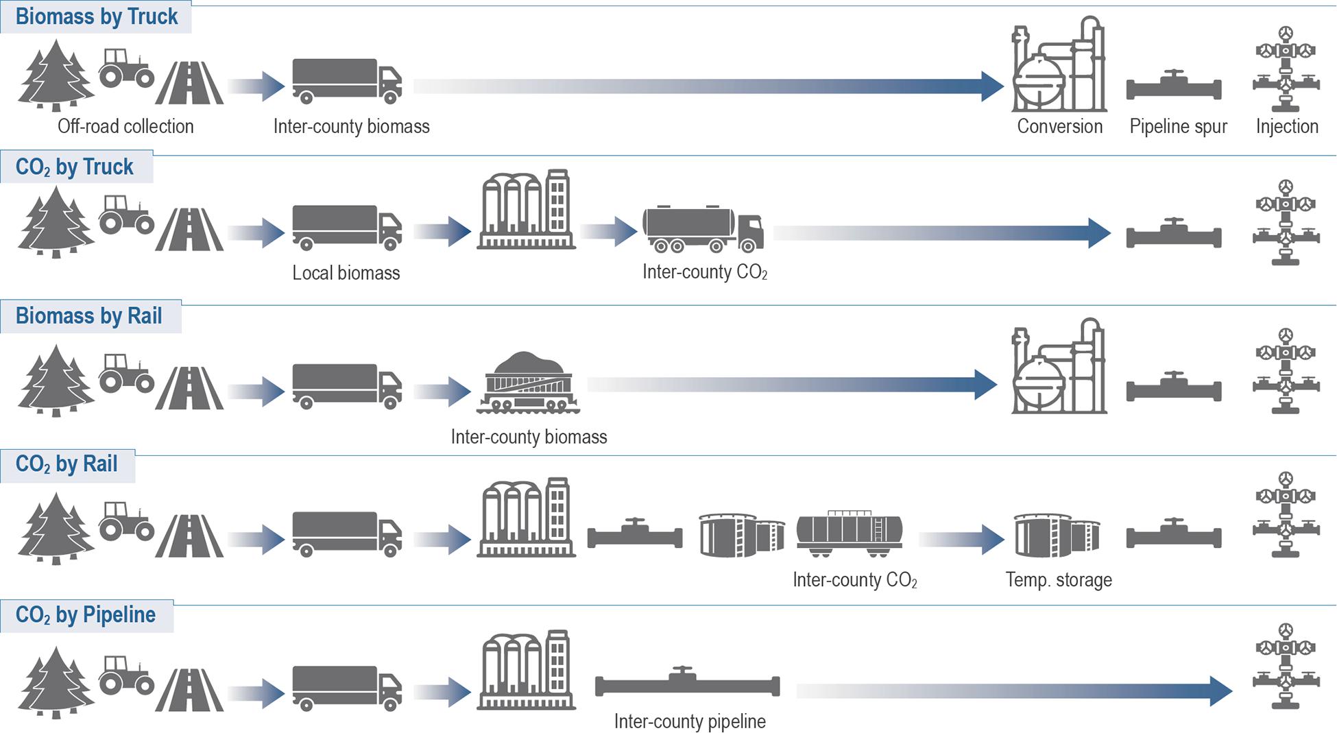
Figure 1. Possible transport configurations for Net Negative Biofuels projects. Inter-county refers to the longer leg of the sequences, while local refers to transport of tens of kilometers.

These scenarios assume that an NNBF facility is sited either near biomass sources or near CO₂ storage, and not at an intermediate distance between. For a single project, and considering transport costs alone, the economic optimum will always be one of these two extremes. However, with permit restrictions, limited rights-of-way, or other practical considerations, a developer may choose an intermediate plant location. In that case, the transport cost can be estimated by a weighted average of the two scenarios. Another case where intermediate siting is preferred is within a network of multiple plants, where CO₂ flows can be combined into a common trunk line. That scenario is beyond the scope of this paper, however, the transport cost prior to the shared trunk line (which is likely to be the larger cost) can be estimated by the methods below.

Biomass Collection

The first step in the carbon chain is collection and pre-treatment of biomass into loads suitable for transport by on-road truck. Representative costs for this stage are shown in Table 1 along with average moisture content of the biomass, which affects transport costs down the line. Collection cost is not the focus of this analysis, be we discuss it here for context.

TABLE 1

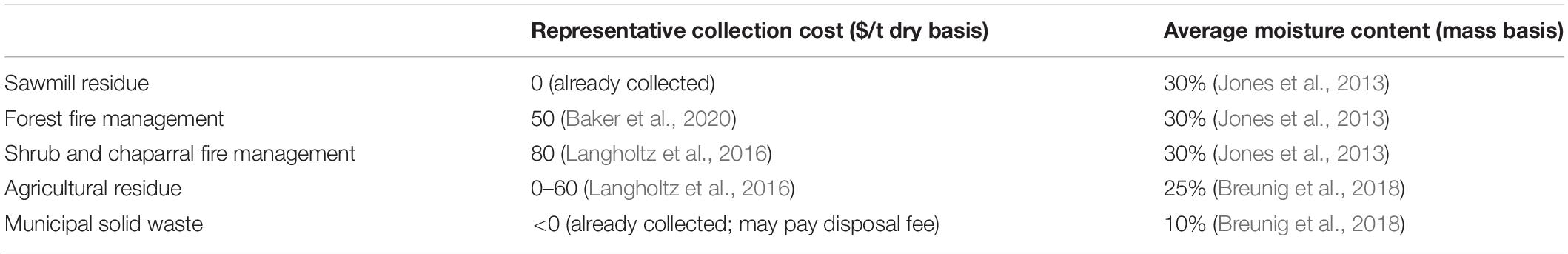
Table 1. Typical collection costs and water content for major categories of waste biomass.

Collection of forest and chaparral residues typically includes chipping and potentially drying before loading trucks at the roadside. For agricultural residues, collection and processing may have already occurred, such as for pistachio shells or almond hulls. As a result, such residues can be purchased at very low additional cost. Other types require collection from the field, so collection cost varies widely. Municipal solid waste (MSW) is already collected by truck and typically already sorted. Biomass from MSW may even be available at negative cost because processing this waste avoids tipping fees at landfills. As described in the Billion-Ton Report (Langholtz et al., 2016), many millions of tons of biomass are available in each of these categories in the United States; any of these types of biomass could support an NNBF project. Supplies are sufficiently concentrated that even a large NNBF plant, say 1 Mt/yr biomass capacity, could, in many places, be supported by a single county supply, or in other cases by several adjacent counties.

Transport of Biomass

From the collection points, biomass will typically be trucked either to a rail station for longer-range transport, or directly to a biomass conversion facility. Trucking is a commodity market with stable prices. Average operating expenses of commercial trucks are surveyed annually by the American Transportation Research Institute (Hooper and Murray, 2018), who reported a national average of $1.05/km in 2017. The cost per ton depends on the load size and capacity factor. We assume that outbound trucks carry 22 tons of biomass, which is close to the legal limit and tracks the average net loads for trucks carrying bulk commodities (National Research Council, 2010). Although there are some agricultural residues that aren’t dense enough to fit 22 t in a standard trailer volume, these can be compacted or otherwise processed to reduce shipping volume. We assume the trucks return empty (50% capacity factor). We also add 6% profit to reflect prices for the project operator (Biery, 2018). The resulting unit cost is shown in Table 2, along with several other unit costs described below.

TABLE 2

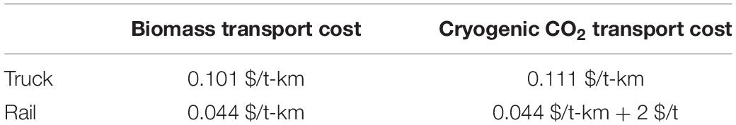
Table 2. Unit costs for truck and rail transport.

Biomass transport by rail is also common in the U.S. as well as internationally. Rail is well known to have lower cost and lower externalities than trucking (GAO, 2011), so it is generally preferred wherever it is available. However, rail access is limited and building new rail spurs is expensive, with representative costs in the range of $0.6–1.2 M/km – somewhat more than for CO₂ pipelines (Compass Int., 2017). Short delivery distances may also favor trucking.

The market for rail transport is more heterogeneous than for trucking. Unit prices vary significantly contract to contract, and average prices vary by about a factor of two depending on the travel distance, load size (number of cars), and type of commodity (Prater and O’Neil, 2014; Mintz et al., 2015). For our base case cost, we assume that transport will be in the short-haul category (<800 km), but with larger loads (>75 cars per train), suggesting a unit cost that is 1.6 times the national average.

Transport of CO₂

Once biomass is transported to the NNBF or BECCS facility, it is processed and treated. The resulting CO₂ is captured and either compressed for transport via pipeline or liquified for transport by truck or rail. Pipeline CO₂ can then be injected directly underground when it reaches the storage site. Liquified CO₂, which is kept at about –40°C and 20 bar of pressure, must be warmed and compressed before injection into a pipeline (80–120 bar and ambient temperature).

Liquified CO₂ can be transported in insulated tanker cars that are similar between truck and rail. We assume the near-full capacity of 22 t is retained for trucks, however, costs are somewhat higher because the trailers are more expensive and the trucks are slightly more expensive to operate and maintain. Survey results give $1.16/km with the adjusted unit cost shown in Table 2.

CO₂ transport by rail is less common than other modes. Although it occurs commercially (ITJ, 2019), we have not found published market data on CO₂ specifically. The costs should be similar to other tanker-shipped commodities, with the exceptions that staging and loading facilities must be built at the origin station, and unloading and reconditioning facilities must be constructed at the destination station. A pipeline spur is likely also needed at the destination.

Two studies have used techno-economic models to estimate the cost of CO₂ by rail for CO₂ storage case studies. Gao et al. (2011) calculated 77 RMB/t-CO₂ ($13/t in 2018 US dollars) to transport 1.5 Mt/yr over 600 km for a project in China. This included $0.88/t for staging and loading facilities. Roussanaly et al. (2017) estimated 4 €/t and 11 €/t ($5 and $13) to transport CO₂ for 50 km and 200 km, respectively, for a project in the Czech Republic. That includes about 1 €/t for loading and unloading facilities. The staging operation thus appears to be a minor part of transport cost. Overall, we assume that the staging and loading operation adds 2 $/t-CO₂ to the cost of transport by rail, while the unit cost remains the same as for biomass.

The cost of CO₂ transport by pipeline is more variable than for other modes since it depends on local construction costs and securing rights of way. Even with these challenges, pipelines are strongly preferred for large volumes of CO₂. There are over 7,000 km of CO₂ pipelines in the U.S. as well as a vastly larger network of natural gas pipelines that also informs the cost of pipeline construction (Wallace et al., 2015).

To estimate CO₂ transport costs via pipeline, we use a spreadsheet-based model developed by the National Energy Technology Laboratory (NETL, 2018), which in turn implements several earlier models from the literature (Parker, 2004; McCoy and Rubin, 2008). When validating the model against recent CO₂ pipeline projects, the authors found that the variant based on Parker tended to overestimate costs, while the variant based on McCoy and Rubin underestimated it. We thus take these to be the upper and lower bounds of the pipeline costs in further analysis. Figure 2 shows results from the model for a 1 Mt/yr CO₂ flow. The McCoy model provides costs for five different regions of the U.S. This yields a cost variation of about +/−20%, whereas the difference between the models can be more than a factor of two. For the generic cost comparisons in Figures 5 and 6, we use the lowest regional result from McCoy (central) and the Parker results as the lower and upper bounds, respectively. For the single-point cost estimates in Figure 7, we use the midpoint between the average of the McCoy estimates and the Parker estimate. The retrieved costs are the break-even cost of CO₂ transport in the first year of operation.

FIGURE 2

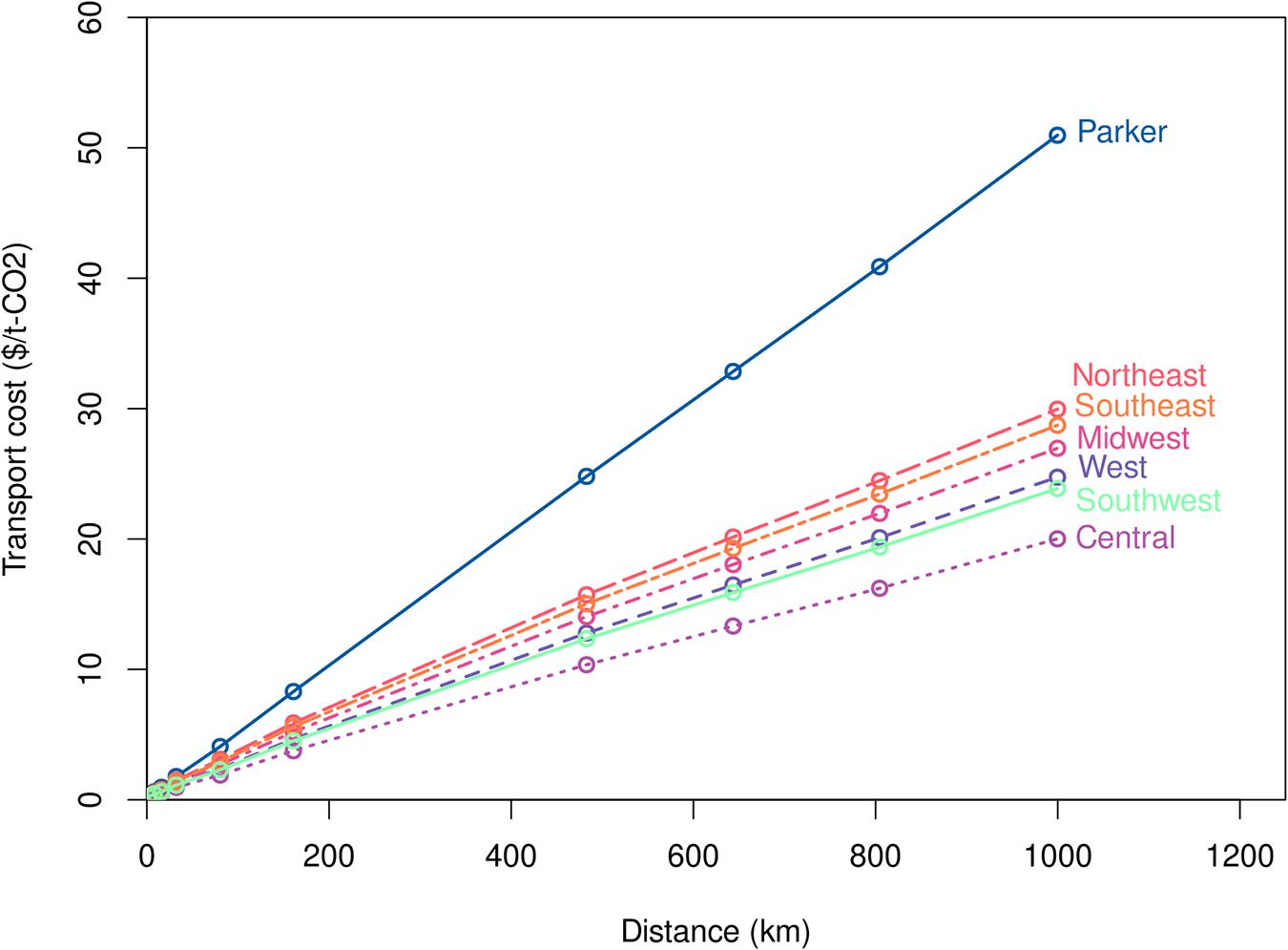
Figure 2. Cost of CO₂ transport by pipeline in the United States by model and region for a flow of 1 Mt/yr in 2014 dollars. “Parker” represents the model with the Parker (2004) variant, and the other lines show results for the McCoy and Rubin (2008) variant for the respective regions of the U.S.

Plant Size and CO₂ Storage Factor

The amount of CO₂ that ultimately ends up in the ground for each ton of biomass collected depends on the BECCS or NNBF technology used, and to a lesser extent, on the type of biomass. To estimate the transport costs per ton of CO₂ stored, we have to account for this “CO₂ storage factor.” Table 3 shows these factors for a handful of likely projects. Most of these plant types are in development in California or neighboring states. The values range from 0.49 t CO₂ per t dry biomass for a pyrolysis to liquid fuels plant, where the majority of biomass carbon ends up in fuel, to 1.6 for gasification to hydrogen, where virtually all the input carbon ends up in the ground. For combustion to electricity, we assume the CO₂ capture system is 90% efficient, a typical benchmark, but it could be made more efficient. Alternatively, some gasification plant designs are less efficient at capturing CO₂ and would have slightly lower values. Project developers can make these choices based on market conditions and regulatory incentives for carbon removal. These storage factors, and thus the costs per ton of CO₂ calculated later, do not account for fossil CO₂ emitted during transport or other life-cycle considerations. However, we previously found transport-related emissions to be less than 1% of the CO₂ stored (Baker et al., 2020).

TABLE 3

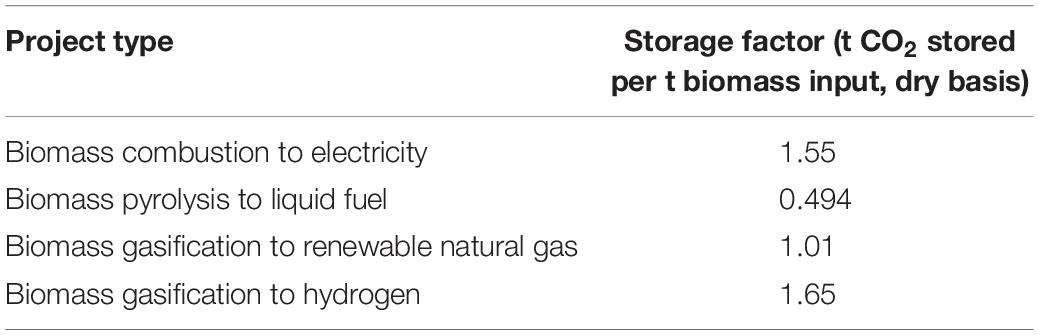
Table 3. CO₂ storage factors for some NNBF and BECCS projects.

Along with the storage factor, the size of the BECCS or NNBF plant determines the flowrate of CO₂ and biomass that must be transported. This affects the cost of pipelines most strongly. In general, larger plants are more economic from a transport perspective. Although not covered here, CO₂ storage cost also depends strongly on CO₂ flowrate. A larger NNBF project may be able to support a dedicated storage project economically; for reference, a single well in a good formation can accept on the order of 1 Mt/yr of CO₂ injection. Smaller projects would likely need to send CO₂ to a storage site that aggregates CO₂ from multiple sources for the best marginal cost. Aggregating CO₂ sources would also be a way to economically transport CO₂ over longer distances by using a shared CO₂ trunk line.

Operating commercial pyrolysis plants are typically small, around a few hundred tons per day of dry biomass (Lee Enterprises Consulting, 2020), though a handful of recently proposed biomass projects without CCS are sized at 1,000 t/d of biomass, such as the Clearfuels gasification plant in Tennessee or the Rialto pyrolysis plant in California, (NETL, 2016). CO₂ capture, transport, and storage would be significantly more expensive at the smaller end of this spectrum. There isn’t enough information on capture costs at small scale (most estimates focus on the much larger power plant scale) to confidently select an optimum size for NNBFs, but a study of CO₂ capture systems for industrial sources predicts steep increases in cost below 0.25 Mt/yr CO₂ for several source types (Herron et al., 2014). As we show below, pipeline transport costs increase sharply below about 0.5 Mt/yr. For these reasons, we find it unlikely that a developer would choose an NNBF project in the hundreds of tons per day size range. As another point of reference, coal gasification plants, a relatively mature technology, are frequently in the size range of 7,000–8,000 t/d coal, illustrating the economies of scale in gasification equipment (NETL, 2016). Altogether, we consider 2,000 t/d biomass as a reasonable reference size. This is the value used in the three case studies described below. This is also a common commercial plant size assumption to meet the cost goal for hydrocarbon fuels production from lignocellulosic biomass proposed by the U.S. Department of Energy (Jones et al., 2013; BETO, 2016).

To maximize the carbon removal potential of pyrolysis to liquid fuels, we assume CO₂ is captured from the off gas of non-condensable gas (NCG) combustion as well as off gas from steam reforming of aqueous phase bio-oil. The storage factor was calculated as 0.494 t CO₂ stored per dry ton biomass input based on a process carbon balance (Li et al., 2017). There is also storable biomass carbon in the biochar, which can be sequestered above ground as a soil amendment. How much of the biochar carbon is stored and for how long depends on the use of the biochar. As a soil amendment the majority of carbon is likely to remain sequestered for over 100 years. We have not included the stored carbon from biochar here, instead focusing on geologically stored CO₂. However, including a stored biochar component would tend to decrease the apparent transport costs per unit of CO₂ removed.

The storage factor for biomass combustion to electricity is derived from the mass balance reported in Jin et al. (2009). Since the modeled combustion facility uses air to combust the biomass, the flue gas contains a significant fraction of nitrogen that must be separated from the CO₂ prior to sequestration. In this case, the CO₂ in the flue gas is assumed to be captured via an amine system (Cansolv) at 90% efficiency (Zoelle et al., 2015). Other process configurations, such as oxy-combustion or indirect combustion of biomass, would result in CO₂-containing streams that could be captured by other technologies not considered here.

The storage factor for biomass gasification to hydrogen is derived from the mass balance reported in Larson et al. (2009). The water-gas shift process to produce hydrogen can be operated to convert nearly all of the carbon in the biomass feedstock ultimately into CO₂; the bulk of this CO₂ is removed from the hydrogen by a refrigerated methanol (Rectisol) process, and is high enough purity after drying for direct sequestration without adding additional capture units, due to the use of an oxygen-blown gasification process.

Finally, the storage factor for biomass gasification to renewable natural gas (RNG) is derived by estimating the fraction of CO₂ in the gas stream before methanation, based on the composition of the CO₂-containing syngas emitted from the gasifier units in Larson et al. (2009) By mass balance, the hydrogen-to-CO ratio in the syngas is adjusted via water-gas-shift to maximize the amount of methane produced, which increases the fraction of CO₂ in the gas stream. The CO₂ is removed prior to methanation by a refrigerated methanol process.

In principle, anaerobic digestion of biomass with CCS is an alternative pathway to net-negative RNG. However, existing anaerobic digestors, such as for manure and wastewater treatment, are small compared to thermochemical plants. This would lead to much higher CO₂ capture and transport costs. These costs could be mitigated with new capture technology and a CO₂ aggregation scheme across sources, but this is a more complex scenario and we don’t consider it here.

Example Projects

To illustrate the transport cost calculation, we select three plausible project configurations from the United States as case studies. Their locations are illustrated in Figure 3. For the first example, we look to California, where Baker et al. (2020) compiled quantities of biomass waste and residues by county. We found some of the largest sources of biomass include the forested counties in the north, foremost Siskiyou County, for potential fire clearing and sawmill residue. Meanwhile, the nearest of the two most favorable geologic storage locations is in the Bay Delta region in the center of the state, especially in San Joaquin County. These areas are marked in Figure 3A. Since the source area is remote from population centers, product transport could be an challenge here. We choose gasification to renewable natural gas as the technology scenario because the RNG can be injected into existing pipelines in Siskiyou county if the plant is sited there.

FIGURE 3

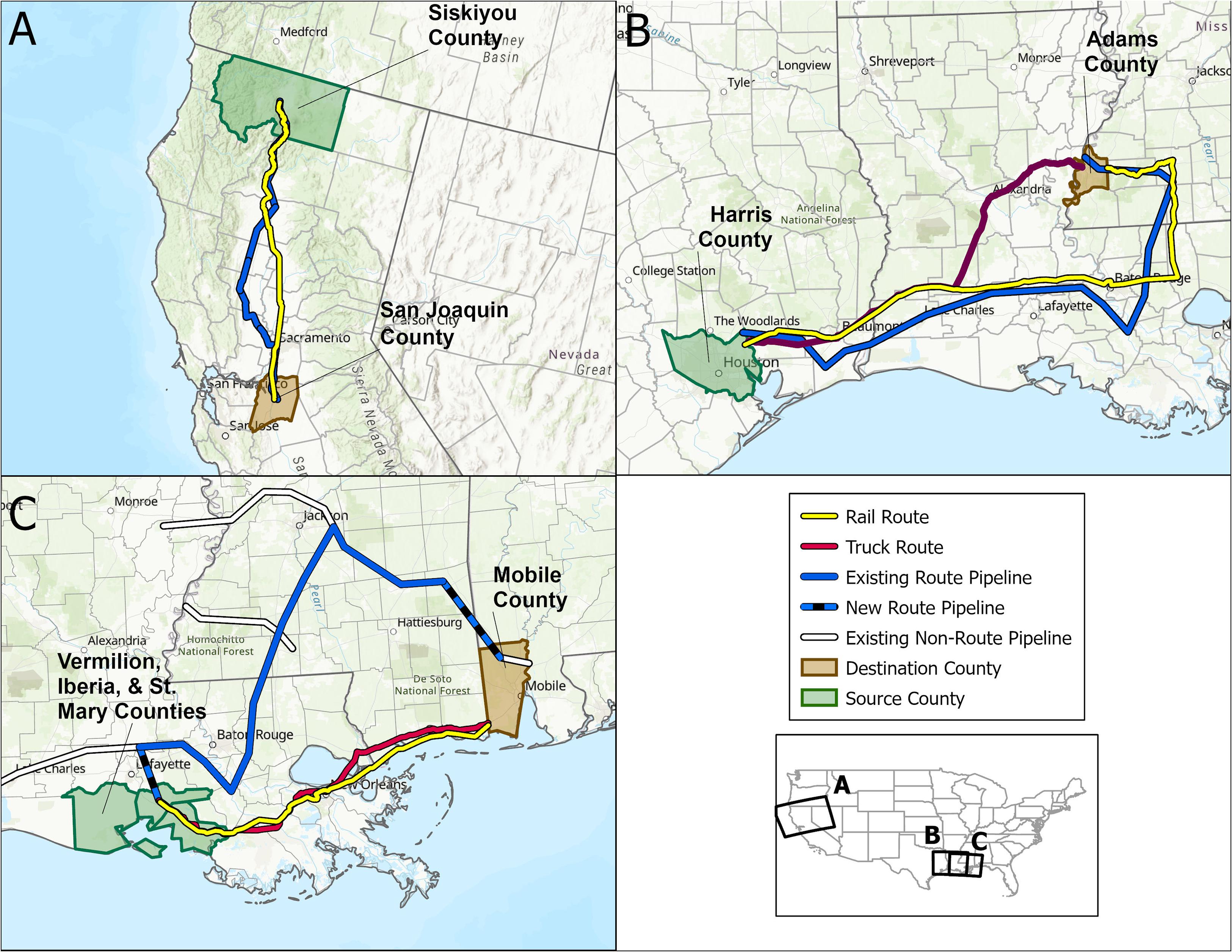
Figure 3. Map of example NNBF project locations showing biomass source areas, CO₂ storage sites, and proposed rail and pipeline routes. (A) Route for forest biomass in Siskiyou County, CA. (B) Route for municipal solid waste from Harris County, TX (including Houston). (C) Route for agricultural residues from Iberia, St. Mary, and Vermilion Counties, LA.

For potential projects outside California, we are not aware of a similar multi-criteria screening for CO₂ storage sites on the national level, though some studies have characterized national storage potential in terms of broad geologic formation and found wide availability (NETL, 2015). CO₂ storage has also been demonstrated in a handful of projects, including two sites in the Gulf Coast region of the U.S. for the SECARB program, which has injected millions of tons of CO₂ for research and demonstration (Foshee, 2010). We use these two proven sites – Natchez, Mississippi (Adams County), and the Citronelle oil field in Mobile County, Alabama – as the CO₂ storage locations in two further scenarios.

The Billion Ton Report (Langholtz et al., 2016) provides biomass waste and residue availability in the United States at the county scale. We surveyed these data in the vicinity of the two storage locations to identify biomass sources large enough to support 2,000 t/d plants. For the second example project, we select municipal solid waste from the highly populated Houston area (Harris County) to be gasified to hydrogen with CO₂ stored in Adams County. The hydrogen can then be sold to one of the many chemical plants or refineries in the region. Incidentally, there is an existing CO₂ pipeline that connects the source and destination counties. If the pipeline could be shared with its current uses, this would undoubtably be the lowest cost transport option. However, for sake of generality, we merely use the pipeline route for distance and calculate costs as if a new pipeline is constructed for the project of the same length.

For the third case study, we select agricultural residue from the region south of Lafayette to be converted by pyrolysis to liquid fuel with the process CO₂ stored in Mobile County. The source counties are relatively small here, so we aggregate biomass from three counties to meet the plant’s demand. For the rail and pipeline scenarios, transport costs are calculated as if the biomass is trucked to a common depot in Iberia County (the center of the three) where it is either processed or transferred to rail to be processed in Mobile County. Again, there is an existing CO₂ pipeline. In this case, it traverses most of the distance between the source and destination counties, but not completely. We add pipeline legs (shown as hatched segments in Figure 3C) to make the final connections. Again, we use the pipeline route only to measure distance and calculate transport cost as if a dedicated pipeline is constructed.

The transport distances for each mode and case study are calculated using ArcGIS following existing rail, road, and CO₂ pipeline networks. In the Siskiyou County case, a hypothetical CO₂ pipeline route was drawn to follow existing major natural gas pipelines (since there are no CO₂ pipelines in the region). For convenience, several of the routes were calculated to the nearest intersection with a county boundary rather than centroid. The difference is minor and is roughly compensated by our choice of destination spur length.

For each scenario, the average local trucking distance is based on the size of the biomass source area:

$d_{local}=\frac{1}{2}\sqrt{A}$

where A is the area of the origin county or set of counties. This approximates the average distance between random points within the area (Talwalker, 2016). The distance from the storage site to a rail station is based roughly on the size of the storage county relative to the rail route shown. The CO₂ storage factors are taken from Table 3.

Total Transport Cost

The transport cost of a project can be estimated by the sum of costs for each leg of the carbon chain, adjusted by the quantity of CO₂ stored. We calculate the costs for the example projects as follows and suggest that these formulae can be applied generally. We define the unit cost, U, as the cost in $/t-km for the mode and product in subscript; for example U_truck,BM is the cost of trucking biomass per t-km. For rail and pipeline, U depends on distance and flowrate.

For the biomass by truck scenario, where the conversion facility is located near the storage site:

$T=\frac{d{U}_{truck,BM}}{\left(1-W_c\right)f_{CO2}}+d_{spur}{U}_{pipeline}$

where T is the total cost in $/t-CO₂ stored, d is the distance between biomass pick up and the conversion plant (typically the longest part of the chain), and d_spur is the length of the short pipeline from the plant to the injection site. W_c is the water content of the biomass and f_CO2 is the storage factor for the type of plant.

For biomass by rail:

$T=\frac{d_{local}{U}_{truck,BM}+d{U}_{rail,BM}}{\left(1-W_c\right)f_{CO2}}+d_{spur}{U}_{pipeline}$

CO₂ by truck:

$T=\frac{d_{local}{U}_{truck,BM}}{\left(1-W_c\right)f_{CO2}}+d{U}_{truck,CO2}$

CO₂ by rail:

$T=\frac{d_{local}{U}_{truck,BM}}{\left(1-W_c\right)f_{CO2}}+d_{spur,1}{U}_{pipeline}+d{U}_{rail,CO2}+d_{spur,2}{U}_{pipeline}$

Where d_spur,1 is the length of the pipeline at the origin station and d_spur,2 is the length at the destination station.

For CO₂ by pipeline:

$T=\frac{d_{local}{U}_{truck,BM}}{\left(1-W_c\right)f_{CO2}}+d{U}_{pipeline}$

These equations are used to calculate the total transport cost for the three example scenarios shown in Table 4. For the CO₂ by rail scenario, we assume that the plant is built near existing rail so that d_spur,1 = 0, but this need not be the case generally.

TABLE 4

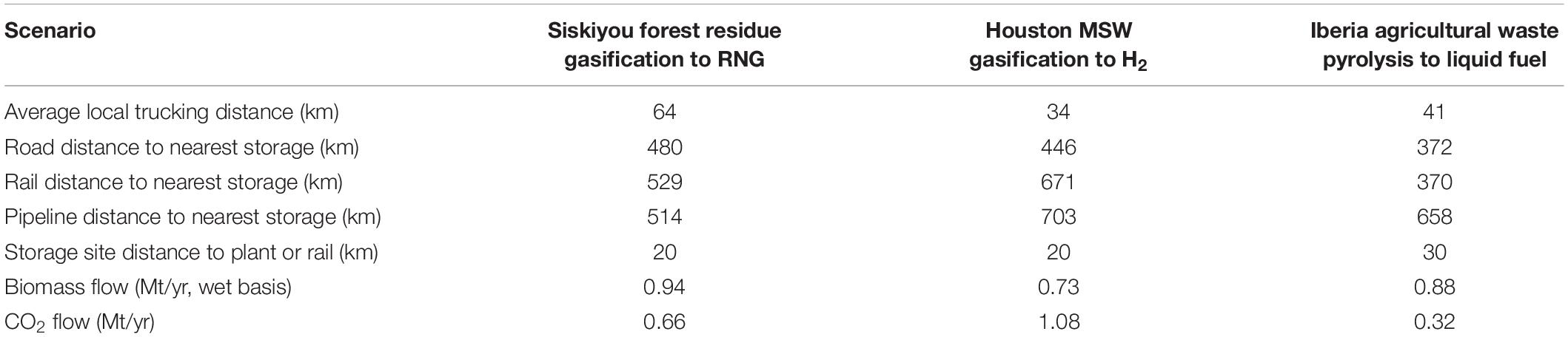
Table 4. Transport characteristics for three example NNBF projects.

Results

The cost of biomass transport by truck and rail is shown in Figure 4. We can see that rail is dramatically less expensive at longer distances. Depending on the project and incentives, biomass could be transported hundreds of kilometers by rail at a reasonable cost. However, trucking has a potential advantage at short distances. For example if biomass is being collected from forests over a large area or many farms in a region, most will not be immediately accessible to rail, so there is a consolidation step by truck. Depending on the average distance between biomass sources and the rail station, direct trucking may have an advantage. With an average truck trip of 30 km to the rail station (reasonable for a biomass-dense area like our example counties), trucks are preferred for a primary distance of about 40 km or less.

FIGURE 4

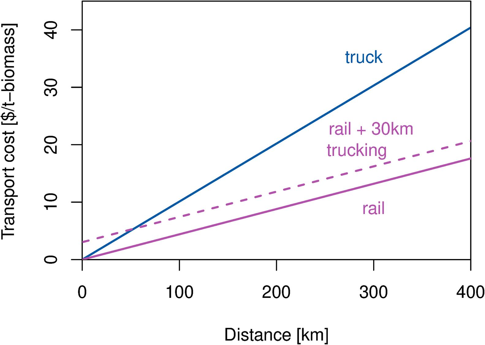
Figure 4. Transport cost of biomass by truck and rail as a function of distance. The dashed line represents a scenario combining consolidation of collected biomass to a rail station via truck (average trip of 30 km) followed by transport by rail for the distance indicated.

The results for transporting CO₂ are shown in Figure 5. In this case, we look at the dependence of the unit cost on CO₂ flowrate, which has a strong effect on pipeline cost and a slight effect on rail cost. This figure shows results for a distance of 200 km, where rail is always preferred to trucking if it is available. At a flowrate of about 1 Mt/yr and above, a pipeline is clearly preferred to rail, and below about 0.3 Mt/yr, rail is clearly the lower cost option. In between those values, the specifics of the project would be needed to determine the best option. These trends are insensitive to distance except at very short distances, where trucking might be preferred to rail for the same reason described above for Figure 4.

Figures 4 and 5 describe the trends for a segment of the transport chain where either biomass or CO₂ must be moved. However, if the site of the NNBF or BECCS plant can be freely selected, then we would like to know whether we should, on the one hand, site the plant near biomass sources and transport CO₂ to the storage site, or on the other hand site the plant near CO₂ storage and transport the biomass. In a biofuel or biomass combustion project without CCS, this isn’t a meaningful choice: the products are easier to transport than biomass and so the plant should be located as close to biomass sources as possible. This consideration also leads to smaller optimum plant sizes. However, with CO₂ transport and storage and their associated economies of scale, the question is more complicated.

FIGURE 5

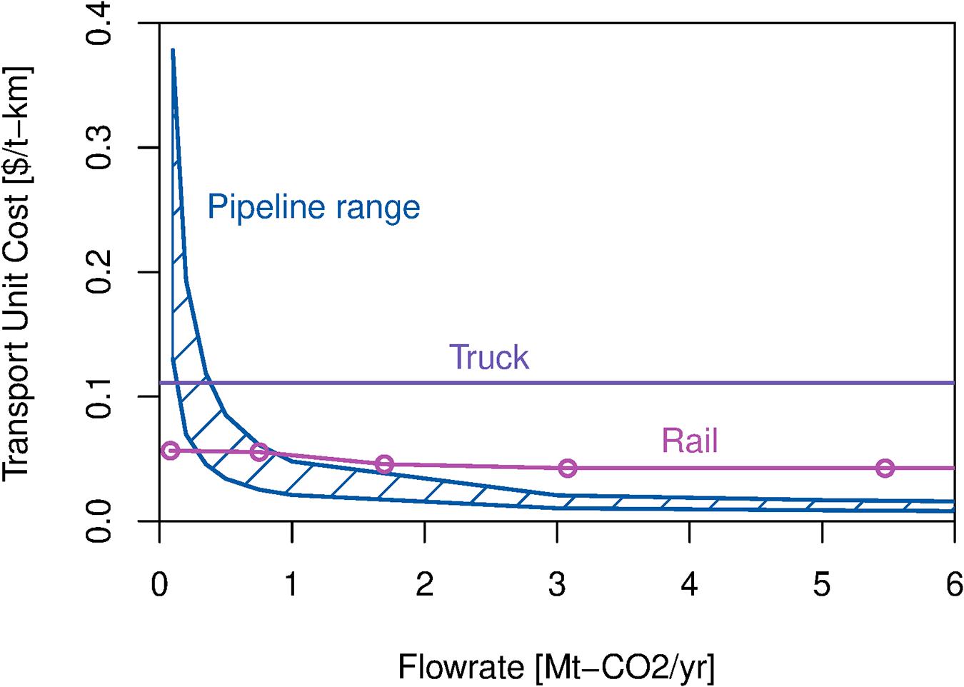
Figure 5. Comparison of transport costs of CO₂ by truck, rail, and pipeline as a function of flowrate. Costs are calculated for a distance of 200 km.

The best choice of plant location depends on the plant size and on the conversion technology being used: specifically, the ratio of CO₂ produced to biomass input. Figure 6 shows the unit costs of the five different modes for a range of the CO₂ storage factor. Triangles under the x-axis mark the values of the factor for the BECCS and NNBF plants listed in Table 3. These factors are not universal; a project developer could always choose to capture less CO₂ (or in some cases slightly more), but the values are constrained by the thermodynamics and stoichiometry of the products and input biomass.

FIGURE 6

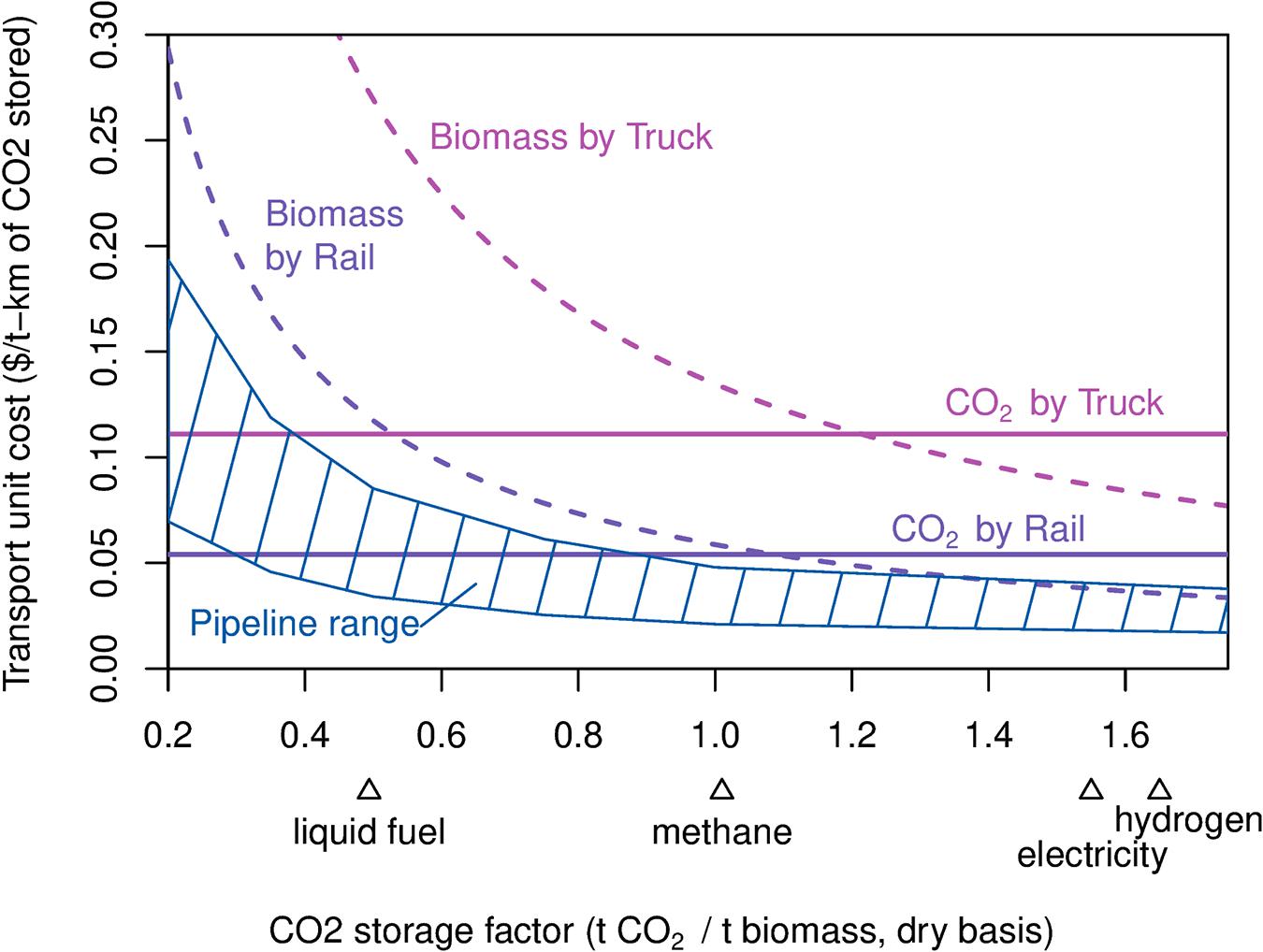
Figure 6. Comparison of transport costs by mode as a function of the CO₂ storage efficiency of the project. Costs are calculated for a biomass input of 1 Mt/yr, dry basis, and 25% water content. Triangles below the x-axis indicate the CO₂ storage factors for several potential project types, as shown in Table 3. Costs reflect the long leg of transport only and neglect local collection and pipeline spurs.

For low storage factors, represented by pyrolysis to liquid fuels, transport of CO₂ is favored over transport of biomass across modes. However, the total volume of CO₂ is low enough that CO₂ by rail competes with a CO₂ pipeline. At a low enough factor, rail is clearly favored because the volume of CO₂ is not enough to make the capital investment in a pipeline worthwhile. However, this depends on the plant size. This figure is calculated for a fixed biomass input of 1 Mt/yr (dry basis). A larger plant would tend to favor a pipeline even at the smaller storage factors, while a smaller plant would favor rail even at higher storage factors. Only the pipeline cost is sensitive to plant size in this way, the relative costs of other modes don’t change much with plant size.

At high storage factors, represented by a gasification to hydrogen project or combustion to electricity, it becomes less expensive to transport biomass by truck or rail than CO₂ by the same mode. The overall volume of CO₂ is large enough that a pipeline is still the lowest-cost option, overall, but this result is sensitive to the plant size. Even at 1 Mt/yr biomass, which is small compared to existing coal gasification plants, but large compared to almost all existing biomass plants, biomass by rail is marginally competitive with a CO₂ pipeline. If constructing a pipeline is not possible due to practical or legal restrictions, biomass by rail appears to be a viable alternative, allowing a developer to bridge hundreds of kilometers of distance between biomass source and geologic storage site for about $10/t of CO₂ stored. This is a modest price compared to the likely cost of capture and to the cost of alternative carbon removal technologies, like direct air capture.

At an intermediate carbon storage factor, such as one achieved by gasification followed by methanation to make renewable natural gas, CO₂ transport by rail and biomass transport by rail are roughly equal cost. CO₂ transport by pipeline is lower cost than both, though again this would change for a significantly smaller plant.

These results suppose that the CO₂ pipeline is dedicated to a single plant. A shared CO₂ pipeline would quickly reduce transport costs and favor the pipeline mode. Indeed, the distance of interest in a project is quite possibly the distance to a shared CO₂ trunk line rather than a storage site. For example, a trunk line which unites the flows of about 9 hydrogen projects of the benchmark size (combined 10 Mt/yr) could move that CO₂ over 1,000 km for $10/t (model average). Geographic opportunities are significantly expanded this way, but a shared CO₂ pipeline also poses challenges of coordination and capacity planning.

The results so far are meant to reveal the general features of the transport problem and mostly apply to the longest segment of the transport chain. To understand the relative importance and the approximate costs of the other segments, we will look at several example projects. The total transport cost can’t be calculated without reference to local distances, proximity to rail, and specifics of the conversion plant. However, we can get some insight by looking at several plausible example projects. Based on our previous study of carbon removal in California and on previous demonstrations of CO₂ storage in the southeastern U.S., we propose three projects that convert biomass waste or residues and store CO₂ in a geologic formation. Locations of the projects and proposed routes are shown in Figure 3.

The calculated distances for components of the five transport scenarios are shown in Table 4 with other characteristics of the example projects. Calculated distances range from 370 km for the Iberia rail route to 700 km for the Houston pipeline route. All three scenarios traverse relatively long distances; the average source-to-storage distance calculated in Baker et al. (2020) was only 70–160 km, depending on biomass type. In a case study matching industrial CO₂ sources to sinks in Pennsylvania, Psarras et al. (2017) found transport distances of 64–140 km. Assessing CO₂ storage from ethanol refineries, Sanchez et al. (2018) found 4 Mt/yr of abatement within 80 km of a storage site across the U.S., however, with sufficient incentives and a shared pipeline network, system average travel distances grew to over 1,000 km. The three scenarios proposed here may inform the bounds of what can be implemented without a shared CO₂ pipeline.

Figure 7 shows the estimated total transport costs for each of the three example projects via each of five modes. For Siskiyou forest biomass, the lowest cost option is to site the plant at the source and transport the CO₂ 530 km by rail to the storage site, giving a total transport cost of $36/t-CO₂ stored. However, this is virtually tied with transporting the CO₂ by pipeline ($37/t); either may be preferred based on the specifics of the project and pipeline route. Note that these costs start at the roadside and do not include collection of the biomass from the forest and grinding. In California, these efforts are likely to be supported by fire-management activities or by commercial timber harvesting, in the case of sawmill residues, but contract prices for biomass will vary.

FIGURE 7

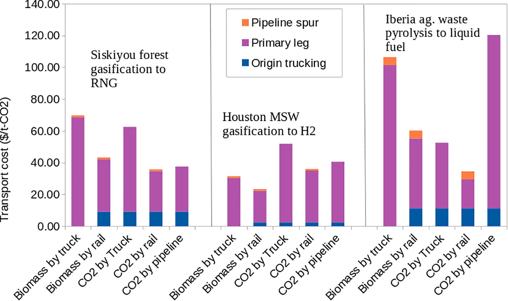
Figure 7. Transport costs by mode for three example projects. Distance varies by each project, as summarized in Table 4.

Transport costs are overall lowest for municipal solid waste from the Houston area. This is because gasification to hydrogen has the highest CO₂ storage factor, making transport less expensive per unit CO₂, and to a lesser extent because MSW has a lower water content. The best option here is to transport the biomass by rail to a plant near the storage site and then move the resulting CO₂ via a short pipeline spur, giving a total transport cost of $24/t-CO₂. However, if the existing CO₂ pipeline could be contracted for this project, it would likely cut the cost of pipeline transport by an order of magnitude, putting the total transport cost for the CO₂ pipeline scenario in the single digits.

The Iberia agricultural waste scenario has the largest truck and pipeline costs. This is because the low CO₂ storage factor for pyrolysis to liquid fuels results in less efficient use of the biomass in the first case and smaller flows of CO₂ in the latter. However, the pyrolysis scenario produces the most valuable co-product (liquid fuel), so transport costs may be offset. The best option for this scenario is to site the biofuel plant in Iberia County and transport CO₂ by rail to Mobile, giving a total transport cost of $34/t-CO₂. This includes pickup of biomass by truck at the farm gate, but not collection from the field and possible pre-treatment for transport (see Table 1 for those).

As noted, there is an existing CO₂ pipeline that covers most of the distance between Iberia and Mobile counties. If project developers can contract to use this pipeline, then only an additional 146 km would need to be constructed (22% of the total route). However, even constructing that length is costly in this scenario because of the small flowrate of CO₂. If using the existing pipeline was free, the pipeline mode would still cost $35/t, slightly more than CO₂ by rail.

Conclusion

We have assessed the transport costs for carbon removal projects based on biomass conversion with carbon capture and storage in the United States. We used publicly available cost data and techno-economic analyses from the literature to compare transport modes and calculate total transport costs for several example projects. Overall, we find that biomass sources and CO₂ storage sites can be connected across several hundred kilometers for costs in the range of $20–40/t-CO₂ if the developer has at least some flexibility in choice of transport mode and type of plant. Reasonable costs can be achieved via rail if a pipeline is not possible, but much longer distances can be spanned if shared CO₂ pipelines are used.

Transport costs are highest for liquid fuel projects and lowest for hydrogen production and large electric plants. This is due to the higher ratio of CO₂ stored per unit biomass in the latter. Also for these projects with high CO₂ storage ratios, transport of biomass by rail becomes a competitive alternative to CO₂ transport by pipeline. For small projects or very low carbon storage factors, CO₂ transport by rail is preferred over constructing a pipeline. For low flowrates and distances less than a few tens of km, trucking may be competitive with rail and pipelines. When rail and pipeline access are not practical, trucking is a viable alternative but at a higher cost.

These results are based on average costs in the United States. However, modal costs vary locally and internationally, especially for pipelines. If used with local unit costs, the formulae given here can be applied to estimate costs and compare modes. The specific crossover points for preferred mode versus plant size or carbon storage factor will change, but the broad trends will apply wherever the cost of order of truck, rail, and pipeline holds.

Our analysis suggests that developers or policymakers who hesitate on carbon removal projects because of the perceived difficulty of building pipelines should strongly consider rail as either a permanent or intermediate alternative. Even large projects can operate on existing infrastructure at a reasonable cost of transport. However, policymakers designing incentives should expect transport costs of up to a few tens of dollars per ton-CO₂ until a shared pipeline system is constructed.

Data Availability Statement

The original contributions presented in the study are included in the article/supplementary material. Further inquiries can be directed to the corresponding author.

Author Contributions

JS conducted analysis and contributed the bulk of text for this manuscript. SP and WL each conducted analysis on biomass conversion technologies and contributed text and strategic direction. HG and SB contributed assessment of biomass characteristics and availability. WK contributed geographic analysis and figures. SB and RA contributed conceptual model design and strategic direction. All authors contributed to the article and approved the submitted version.

Funding

This study was made possible by support of the Livermore Laboratory Foundation and the ClimateWorks Foundation. This document may contain research results that are experimental in nature, and neither the United States Government, any agency thereof, Lawrence Livermore National Security, LLC, nor any of its employees makes any warranty, express or implied, or assumes any legal liability or responsibility for the accuracy, completeness, or usefulness of any information, apparatus, product, or process disclosed, or represents that its use would not infringe privately owned rights. Reference to any specific commercial product, process, or service by trade name, trademark, manufacturer, or otherwise does not constitute or imply an endorsement or recommendation by the U.S. Government or Lawrence Livermore National Security, LLC. The views and opinions of authors expressed herein do not necessarily reflect those of the U.S. Government or Lawrence Livermore National Security, LLC and will not be used for advertising or product endorsement purposes (Release number: LLNL-JRNL-817853).

Conflict of Interest

The authors declare that the research was conducted in the absence of any commercial or financial relationships that could be construed as a potential conflict of interest.

Acknowledgments

We acknowledge valuable insights and past contributions from our many coauthors on the Getting to Neutral Report (Baker et al., 2020), as well as Matthew Langholtz at Oak Ridge National Laboratory.

References

Baik, E., Sanchez, D. L., Turner, P. A., Mach, K. J., Field, C. B., and Benson, S. M. (2018). Geospatial analysis of near-term potential for carbon-negative bioenergy in the United States. Proc. Natl. Acad. Sci. U.S.A. 115, 3290–3295. doi: 10.1073/pnas.1720338115

PubMed Abstract | CrossRef Full Text | Google Scholar

Baker, S. E., Stolaroff, J. K., Peridas, G., Pang, S. H., Goldstein, H. M., Lucci, F. R., et al. (2020). Getting to Neutral: Options for Negative Carbon Emissions in California. LLNL-TR-796100. Livermore, CA: Lawrence Livermore National Laboratory.

Google Scholar

BETO (2016). Energy department announces $11.3 Million available for mega-bio: bioproducts to enable biofuels. Washington, DC: U.S. Department of Energy. Available online at: https://www.energy.gov/eere/bioenergy/articles/energy-department-announces-113-million-available-mega-bio-bioproducts (accessed February 8, 2016).

Google Scholar

Biery, M. E. (2018). Profit margins for trucking companies on the rise. Am. Trucker Available online at: https://www.trucker.com/business/profit-margins-trucking-companies-ris (accessed April 7, 2021).

Google Scholar

Breunig, H. M., Huntington, T., Jin, L., Robinson, A., and Scown, C. D. (2018). Temporal and geographic drivers of biomass residues in California. Resour. Conserv. Recycl. 139, 287–297. doi: 10.1016/j.resconrec.2018.08.022

CrossRef Full Text | Google Scholar

Charm Industrial (2021). FAQs. Frequently Asked Questions. San Francisco, CA: Charm Industrial.

Google Scholar

Clean Energy Systems (2021). Carbon-Negative Energy; An Opportunity for California. Rancho Cordova, CA: Clean Energy Systems.

Google Scholar

Compass Int. (2017). 2017 Railroad Engineering & Construction Cost Benchmarks. The Villages, FL: Compass International Inc.

Google Scholar

Consoli, C. (2019). Bioenergy and Carbon Capture and Storage. Melbourne, VIC: Global CCS Institute.

Google Scholar

Cox, J. (2021). Biofuel project proposed in mcfarland would bury carbon from ag waste, produce alternative to diesel. Bakersf. Californ. 10:2021.

Google Scholar

Creutzig, F., Ravindranath, N. H., Berndes, G., Bolwig, S., Bright, R., Cherubini, F., et al. (2015). Bioenergy and climate change mitigation: an assessment. GCB Bioener. 7, 916–944. doi: 10.1111/gcbb.12205

CrossRef Full Text | Google Scholar

Foshee, T. (2010). SECARB: Southeast Regional Carbon Sequestration Partnership. Available obline at: https://www.sseb.org/programs/secarb/ (accessed May 24, 2010).

Google Scholar

Gao, L., Fang, M., Li, H., and Hetland, J. (2011). Cost analysis of CO2 transportation: case study in China. Energy Procedia 4, 5974–5981. doi: 10.1016/j.egypro.2011.02.600

CrossRef Full Text | Google Scholar

GAO (2011). Surface Freight Transportation A Comparison of the Costs of Road, Rail, and Waterways Freight Shipments That Are Not Passed on to Consumers. Washington, DC: United States Government Accountability Office.

Google Scholar

Helena, C., Faaij, A., Moreira, J., Berndes, G., Dhamija, P., Dong, H., et al. (2011). “Bioenergy,” in IPCC Special Report on Renewable Energy Sources and Climate Change Mitigation. (Cambridge: Cambridge University Press). Available online at: https://www.ipcc.ch/report/renewable-energy-sources-and-climate-change-mitigation/

Google Scholar

Herron, S., Zoelle, A., and Summers, W. (2014). Cost of Capturing CO₂ From Industrial Sources. Pittsburgh, PA: National Energy Technology Laboratory. Available online at: https://www.netl.doe.gov/energy-analysis/details?id=1836

Google Scholar

Hooper, A., and Murray, D. (2018). An Analysis of the Operational Costs of Trucking: 2018 Update. New York, NY: ATRI.

Google Scholar

ITJ (2019). CO2 transport by rail reduces greenhouse gas emissions. Int. Trans. J. Available obline at: https://www.transportjournal.com/en/home/news/artikeldetail/co2-transport-by-rail-reduces-greenhouse-gas-emissions.html (accessed September 12, 2019).

Google Scholar

Jin, H., Larson, E. D., and Celik, F. E. (2009). Performance and cost analysis of future, commercially mature gasification-based electric power generation from switchgrass. Biofuels, Bioprod. Bioref. 3, 142–173. doi: 10.1002/bbb.138

CrossRef Full Text | Google Scholar

Jones, S., Meyer, P., Snowden-Swan, L., Padmaperuma, A., Tan, E., Dutta, A., et al. (2013). Process Design and Economics for the Conversion of Lignocellulosic Biomass to Hydrocarbon Fuels: Fast Pyrolysis and Hydrotreating Bio-Oil Pathway. Richland, WA: Pacific Northwest National Laboratory.

Google Scholar

Langholtz, M. H., Stokes, B. J., and Eaton, L. M. (2016). 2016 Billion-Ton Report: Advancing Domestic Resources for a Thriving Bioeconomy Volume 1: Economic Availability of Feedstocks. Washington, DC: U.S. Department of Energy.

Google Scholar

Larson, E. D., Jin, H., and Celik, F. E. (2009). Large-scale gasification-based coproduction of fuels and electricity from switchgrass. Biof. Bioprod. Bioref. 3, 174–194. doi: 10.1002/bbb.137

CrossRef Full Text | Google Scholar

Lee Enterprises Consulting (2020). Pyrolysis Oil – Commercial Markets Are a Reality. Lee Enterprises Consulting, Inc. Available online at: https://lee-enterprises.com/pyrolysis-oil-commercial-markets-are-a-reality/ (accessed July 6, 2020).

Google Scholar

Li, W., Dang, Q., Smith, R., Brown, R. C., and Wright, M. M. (2017). Techno-economic analysis of the stabilization of bio-oil fractions for insertion into petroleum refineries. ACS Sustainable Chem. Eng. 5, 1528–1537. doi: 10.1021/acssuschemeng.6b02222

CrossRef Full Text | Google Scholar

Masson-Delmotte, V., Zhai, P., Portner, H. O., Roberts, D., Skea, J., Shukla, P. R., et al. (2018). “Global warming of 1.5 C. An IPCC Special report on the impacts of global warming of 1.5 C above pre-industrial levels and related global greenhouse gas emissions pathways,” in The Context of Strengthening the Global Response to the Threat of Climate Change, Sustainable Development, and Efforts to Eradicate Provetry, eds M. I. Gomis, E. Lonnoy, T. Maycock, M. Tignor, and T. Waterfield, (Geneva: World Meteorological Organization).

Google Scholar

McCoy, S. T., and Rubin, E. S. (2008). An engineering-economic model of pipeline transport of CO2 with application to carbon capture and storage. Int. J. Greenh. Gas Control 2, 219–229. doi: 10.1016/S1750-5836(07)00119-3

CrossRef Full Text | Google Scholar

Mintz, M., Saricks, C., and Vyas, A. (2015). Coal-by-Rail: A Business-as-Usual Reference Case. ANL/ESD-15/6. Chicago, IL: Argonne National Laboratory.

Google Scholar

Minx, J. C., Lamb, W. F., Callaghan, M. W., Fuss, S., Hilaire, J., Creutzig, F., et al. (2018). Negative emissions- Part 1: reseach landscape and synthesis. IOP Publish. Ltd 13, 1–29. doi: 10.1088/1748-9326/aabf9b

CrossRef Full Text | Google Scholar

National Academies of Sciences, Engineering, and Medicine (2019). Negative Emissions Technologies and Reliable Sequestration: A Research Agenda (2019). Washington, DC: National Academies of Sciences, Engineering. doi: 10.17226/25259

PubMed Abstract | CrossRef Full Text | Google Scholar

National Research Council (2010). Technologies and Approaches to Reducing the Fuel Consumption of Medium- and Heavy-Duty Vehicles. Washington DC: The National Academies Press.

Google Scholar

NETL (2015). Carbon Storage Atlas, 4 Edn. Pittsburgh, PA: National Energy Technology Laboratory.

Google Scholar

NETL (2016). Gasification Plant Databases. Pittsburgh, PA: National Energy Technology Laboratory.

Google Scholar

NETL (2018). FE/NETL CO2 Transport Cost Model: Description and User’s Manual DOE/NETL-2018/1877. Pittsburgh, PA: National Energy Technology Laboratory.

Google Scholar

Onyebuchi, V. E., Kolios, A., Hanak, D. P., Biliyok, C., and Manovic, V. (2018). A Systematic review of key challenges of CO2 transport via pipelines. Renew. Sustain. Ener. Rev. 81, 2563–2583. doi: 10.1016/j.rser.2017.06.064

CrossRef Full Text | Google Scholar

Parker, N. (2004). Using Natural Gas Transmission Pipeline Costs to Estimate Hydrogen Pipeline Costs. UCD-ITS-RR-04-35. Davis, CA: Institute of transportation Studies.

Google Scholar

Prater, M., and O’Neil, D. Jr. (2014). Rail Tariff Rates for Grain by Shipment Size and Distance Shipped. Washington, DC: United States Department of Agriculture.

Google Scholar

Psarras, P. C., Comello, S., Bains, P., Charoensawadpong, P., Reichelstein, S., and Wilcox, J. (2017). Carbon capture and utilization in the industrial sector. Environ. Sci. Technol. 51, 11440–11449. doi: 10.1021/acs.est.7b01723

PubMed Abstract | CrossRef Full Text | Google Scholar

Rosenfeld, J., Kaffel, M., Lewandrowski, J., and Pape, D. (2020). The California Low Carbon Fuel Standard: Incentivizing Greenhouse Gas Mitigation in the Ethanol Industry. Washington, DC: USDA, Office of the Chief Economist.

Google Scholar

Roussanaly, S., Skaugen, G., Aasen, A., Jakobsen, J., and Vesely, L. (2017). Techno-economic evaluation of CO2 transport from a lignite-fired IGCC plant in the Czech Republic. Int. J. Greenh. Gas Control 65, 235–250. doi: 10.1016/j.ijggc.2017.08.022

CrossRef Full Text | Google Scholar

Sanchez, D. L., Johnson, N., McCoy, S. T., Turner, P. A., and Mach, K. J. (2018). Near-term deployment of carbon capture and sequestration from biorefineries in the united states. Proc. Natl. Acad. Sci. U.S.A. 115, 4875–4880. doi: 10.1073/pnas.1719695115

PubMed Abstract | CrossRef Full Text | Google Scholar

Talwalker, P. (2016). Distance between two random points in a square – sunday puzzle. Mind Your Decis. (Blog) Available online at: https://mindyourdecisions.com/blog/2016/07/03/distance-between-two-random-points-in-a-square-sunday-puzzle/ (accessed July 3, 2016).

Google Scholar

Wallace, M., Goudarzi, L., and Wallace, R. (2015). A Review of the CO2 Pipeline Infrastructure in the U.S.” DOE/NETL-2014/1681. Pittsburgh, PA: National Energy Technology Laboratory.

Google Scholar

Zoelle, A., Keairns, D., Pinkerton, L. L., Turner, M. J., Woods, M., Kuehn, N., et al. (2015). Cost and Performance Baseline for Fossil Energy Plants Volume 1a: Bituminous Coal (PC) and Natural Gas to Electricity Revision 3.” Technical Report DOE/NETL-2015/1723. Pittsburgh, PA: National Energy Technology Laboratory.

Google Scholar