The PESERA-DESMICE Modeling Framework for Spatial Assessment of the Physical Impact and Economic Viability of Land Degradation Mitigation Technologies

Introduction

Land degradation, the human-induced reduction or loss of the biological or economic productivity and complexity of agro-ecosystems (UNCCD, 1994), is a pressing development problem of global dimensions. It occurs through a variety of processes such as soil erosion by wind and/or water, deterioration of the physical, chemical, and biological or economic properties of soil, or long-term loss of natural vegetation. Over time, a plethora of sustainable land management (SLM) measures have evolved or were actively designed by land users and other stakeholders to mitigate the land degradation challenge. The academic community has similarly developed multiple approaches to assess the impacts of land degradation (cf. Turner et al., 2016). Among these, computer modeling is one of the most versatile as it allows to combine multiple drivers in scenario assessments at low cost. Scale has been an important consideration in developing such models, especially in conceptualizing the feedbacks between natural and human systems.

Soil erosion models date back several decades: frequently these are comprehensive process-based models requiring detailed input data, while others are empirically derived models that are difficult to transfer. The PESERA model (Kirkby et al., 2008), originally developed for Pan-European Soil Erosion Risk Assessment within a dedicated EU (FP5) project, is a rare attempt to develop a process-based regional scale approach that can be run with relatively limited input data. Not only is the regional scale interesting to contrast erosion processes across landscapes, but the individual grid cell resolution of 100 m–1km, coincides with the field scale and may be conceived as the basic land management unit. For land managers and policy makers, the critical question is not to assess land degradation itself, but the effectiveness of SLM measures to mitigate the problem. Within the DESIRE project, a cyclical approach was operationalized involving the design, trialing, and evaluation of multi-stakeholder, multi-scale strategies to combat desertification (Reed et al., 2011). For upscaling and scenario assessment of these strategies, the PESERA model was embedded in a newly developed PESERA-DESMICE (Desertification Mitigation Cost-Effectiveness) modeling framework.

Site-selection modeling for optimization of conservation efforts is a well-established research area for biodiversity conservation (e.g., Camm et al., 1996; Crossman et al., 2007; Tulloch et al., 2014), but has so far rarely been applied to the mitigation of land degradation (see e.g., Forouzangohar et al., 2014). This research will enable landscape-scale assessments of the most cost-effective ways to attain environmental targets. Furthermore, although cost-benefit analysis (CBA) is an established method in evaluating soil and water conservation measures, from individual measures (de Graaff, 1996; Ludi, 2004; Fleskens et al., 2005, 2007; Posthumus and de Graaff, 2005) to projects (de Graaff, 1996; Ninan and Lakshmikanthamma, 2001) to continental and global scales (Pimentel et al., 1995; Kuhlman et al., 2010), so far the spatial variability of the profitability of SLM measures has received little attention (see e.g., Birch et al., 2010; Evans et al., 2015). The model described in this report offers a method which considers the perspective of both individual land users and policy makers, and can scale up results from the field to the region and beyond.

Linking environmental and socio-economic models facilitates a spatially explicit evaluation of mitigation strategies. By selecting the most financially attractive option available at grid cell level, the economic model informs a realistic spatial configuration of the adoption potential of measures by individual land users. The coupled models can be used to model environmental (e.g., climate change) as well as socio-economic (e.g., policy) scenarios. The fact that this is done for multiple study areas based on data gathered by a collective effort between researchers and local stakeholders makes the approach truly unique.

Within the DESIRE project, the PESERA-DESMICE framework looks at the biophysical effects and their transformation into economic impacts of different SLM technologies that were selected with local stakeholders (Schwilch et al., 2009) and trialed in experimental sites within each study area (Jetten and Shrestha, 2012). After local calibration the PESERA model was subsequently used to expand the results of these trials to a larger hinterland, in order to evaluate the financial feasibility of these SLM measures across the entire study site. This paper presents and demonstrates the implementation and use of the PESERA-DESMICE assessment framework for spatially-explicit evaluation of the biophysical impacts and financial viability of desertification mitigation measures. In the next sections, it first introduces the set-up of the modeling framework (see Section The PESERA-DESMICE Modelling Framework), then illustrates its use for three case study sites (see Section Illustrative Model Applications), and finally offers a discussion and conclusions (see Sections Discussion and Conclusions).

The PESERA-DESMICE Modeling Framework

PESERA-DESMICE Model Overview

This section outlines the PESERA-DESMICE modeling approach. The PESERA model (Kirkby et al., 2008) is a process-based model, originally developed primarily for soil erosion assessment. In the context of the DESIRE project, this model has been adapted and expanded to evaluate the broader biophysical consequences of alternative land degradation remediation strategies (Kirkby et al., 2010). According to the WOCAT¹ terminology, remediation strategies consist of technologies and approaches. A technology can consist of a single or multiple of four types of measures: structural, vegetative, agronomic, and management measures, respectively (Liniger and Critchley, 2007). The PESERA-DESMICE framework embeds PESERA in a sequence of six logical steps in which the impact and feasibility of SLM technologies are directly assessed (see also Figure 1):

FIGURE 1

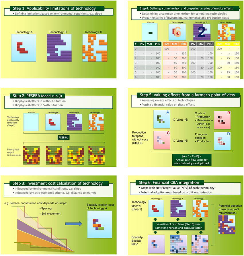
Figure 1. The six steps of the PESERA-DESMICE modeling approach (DESMICE framework in which a PESERA model run is embedded).

Step 1: Technology Applicability Limitations

First it is necessary to define where each technology can in principle be applied. Limitations as meant here are physical constraints, rather than factors reducing expectations that the technology will be cost-efficient. This is an important step in that it rules out the area where technologies cannot be applied—e.g., terraces on steep slopes with shallow soils. Factors considered include: soil depth, slope, landform, land use, climate, and distance to streams. For each technology, each of the above criteria will result in an output map showing the applicability in a dichotomous fashion. Only when all applicability limitations of a technology are satisfied can the technology be applied in a certain area.

Step 2: PESERA Model Runs

The physical effects of implementing the technology can now be evaluated using the PESERA model. This is done separately for each technology, taking into account its potential applicability area (step 1). To evaluate each technology, two model assessments need to be made: first a baseline run without remedial technologies, and then a separate adapted run for each technology applied separately, to provide the biophysical changes for substitution into the DESMICE economic assessment, thus providing a before and after comparison.

Step 3: Investment Cost Calculation

The WOCAT technology questionnaires in most cases present a generalized cost estimate of the technology. In reality, construction, and maintenance costs will differ based on environmental factors (e.g., slope) and socio-economic factors (e.g., distance to market). In this step, costs are made spatially explicit by considering both types of factors. Environmental variation is implemented by using technology-specific rules linking the standard quantities per input category contained in the WOCAT database to the environmental conditions in each grid cell. The distance to market functionality was included in DESMICE as an option but not implemented for DESIRE study sites. It allows defining for each cost item the location of source areas (markets) and transportation costs. Multiplying spatially-explicit inputs with their respective spatially-explicit costs gives the total investment or annual maintenance cost.

Step 4: Defining a Time Horizon and Preparing a Series of On-Site Effects

The technologies that are being assessed may have different economic lifetimes. Therefore, shorter-lived technologies are assessed over several cycles of re-investment (over the length of time that the longest lived technology is likely to last for). Years of (re-)investment are filled first; maintenance costs are subsequently added for years in between investment. Production costs need also to be considered because application of technologies may lead to a change of land use or use of input (e.g., more labor because of larger harvest).

Step 5: Valuing Effects from a Farmer's Point of View

To value effects of a remediation strategy, evolution of the following will be assessed on a yearly basis for the lifetime of the technology (or multiple lifetimes):

A. Production output (yield x value);

B. Costs of implementing the technology and land use associated with it;

C. Production output (yield x value) as it would develop were the mitigation strategy not applied;

D. Costs of the land use in the case without mitigation.

For each year, the net financial result of implementing a remediation strategy can then be calculated as the output achieved with the technology minus the costs associated with its implementation, minus foregone benefits in the case without mitigation and adding foregone costs of that without case, i.e.,: [A−B−C+D] (note that benefits and costs may vary both in space and time).

Step 6: Financial CBA Integration

The annual cash-flows of step 5 are subsequently used in a Financial Cost-Benefit Analysis (FCBA). An important issue in FCBA is discounting, i.e., introducing an interest rate that depreciates costs or benefits occurring in the future relative to those felt now. Summing discounted cash-flows gives the Net Present Value (NPV) for each technology. For each grid cell, one of the following three possible outcomes will apply:

• The technology with highest NPV will be selected (when positive; the adoption grid in Figure 1 shows a possible configuration of technology A, B, and C).

• No technology will be selected if all NPVs are negative (i.e., white pixels in potential adoption grid).

• No technology will be selected if no technology is applicable in the area (blue cells in adoption grid).

Scenario Development

Once the steps 1–6 have been followed, PESERA-DESMICE can be used to run different scenarios. Scenarios can include specific approaches to upscaling of technologies. In the DESIRE project, scenarios included: (i) policy scenarios to assess the effectiveness of financial incentive (and alternative) mechanisms to stimulate adoption of technologies if they are not economically attractive; and (ii) two so-called “global” scenarios with the objective to maximize food production and minimize land degradation, respectively. The food production scenario selects the technology with the highest agricultural productivity (biomass) for each cell where a higher productivity than in the baseline scenario is achieved. The minimizing land degradation scenario selects the technology with the highest mitigating effect on land degradation or none if the baseline situation demonstrates the lowest rate of land degradation. Further, details about the scenario assessment are provided in Fleskens et al. (2014).

Assessing Additional Degradation Processes

The PESERA model was originally conceived to assess soil erosion by water. Within the DESIRE project, the model was extended to more effectively capture the role of grazing, fire, and wind erosion as drivers of degradation. These degradation processes were targeted as they were identified as common drivers of desertification in the respective DESIRE study sites (Hessel et al., 2014). Soil erosion by water is globally the most severe threat to soils (Montanarella et al., 2016). Recent high-resolution model analysis estimates that 24% of the European land area suffers unsustainable soil losses due to water erosion (Panagos et al., 2015a). Overgrazing is an important cause of land degradation in rangelands, with severe impact in e.g., Mongolia (Hilker et al., 2014) and Botswana (Perkins et al., 2013). Loss of grassland net primary productivity data presented by Gang et al. (2014) suggests 7% of European land area experiences grassland degradation. Large-scale assessment of overgrazing is however hampered by lack of data on vegetation dynamics (e.g., proliferation of unpalatable species). Fires occur naturally in many dryland ecosystems, but can cause large-scale disturbances and degradation in landscapes strongly altered by humans, such as in the Mediterranean basin (Pausas et al., 2008). About 0.5 Mha is burnt annually in Europe, and this is projected to increase due to climate change (Khabarov et al., 2016). Data from Schmuck et al. (2015) suggests that over the past 25 years, close to 3% of the European land area has been burnt. Despite important gaps in knowledge about the severity of wind erosion (Stolte et al., 2015), it was recently estimated that over 8% of the European land area suffers moderate to high susceptibility to wind erosion (Borrelli et al., 2014). Considering these additional drivers in PESERA furthermore allows considering interdependencies between degradation processes (Stolte et al., 2015) in an integrated way. Apart from capturing additional drivers of degradation, pedotransfer functions were enhanced on the basis of dialogue and data within each study area. This section explains how these changes were conceptualized. As indicated in Section PESERA-DESMICE Model Overview, both the PESERA baseline and adapted PESERA assessment rely on an accurate representation of the locally occurring degradation processes and mitigation options in order to feed output to the DESMICE model. Input requirements for PESERA are detailed elsewhere (Kirkby et al., 2008). The model outputs are summarized in Table 1.

TABLE 1

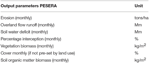
Table 1. Typical output variables for each cell in the PESERA model (Kirkby et al., 2008).

Grazing and Fuel Wood Harvesting

Grazing animals consume vegetation, removing a significant fraction of the primary production. Although a fraction of this consumption (ca. 10%) is returned locally as solid or liquid excretion, there is a net loss of biomass (including carbon and nitrogen) from the system, much of it returned to the atmosphere as CO₂ or CH₄ (methane) and about 10% converted to body tissue (National Research Council, 2000) and finally transferred to market. Figure 2 schematically represents how grazing is included in PESERA. Under equilibrium conditions there is a fairly constant ratio between biomass consumed and the carrying capacity of the land, with transitional states where there is a change in grazing intensity.

FIGURE 2

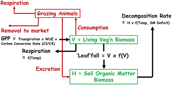
Figure 2. Inclusion of grazing animals within the carbon cycling scheme in PESERA.

The approach adopted has been to specify the fraction of the plant biomass that is consumed each month, which can range from 0 to 100%. This has been preferred to setting the number of grazing animals, as it prevents the possibility of consuming more biomass than is present at any time. As a result the carrying capacity changes through the year. When this approach is implemented in PESERA, we see an interesting relationship between grazing intensity and carrying capacity. At low grazing pressures, increased consumption allows higher carrying capacities but, beyond an optimum, the increased grazing reduces the biomass so much that carrying capacity falls, setting a clear point beyond which the area can be described as “over-grazed.”

Since fuel wood harvesting can also be seen as a removal of a fraction of the biomass, the same approach as for grazing can be used. Accordingly, the code has been modified to recognize that part of the biomass removed can be assigned to animal grazing and another part to fuel wood collection. In spatial analyses, the intensities of removal may be linked to location—e.g access to water for grazing and proximity to cities and roads for fuel wood collection (Perkins et al., 2013).

Fire

We have implemented a simplified fire model within PESERA, using simplified versions of algorithms developed and tested independently (Venevsky et al., 2002) for Portugal. A fire danger index (FDI) is calculated as:

$\begin{array}{ll}FDI=1-\frac{1}{\lambda N}\left[1-\text{exp}(-\lambda N)\right]& (1)\end{array}$

where λ = 0.00037 and

$\begin{array}{ll}N=\overline{T}\left(T_E∕2+4\right)D_{>3}& (\mathrm{1a})\end{array}$

Where $\overline{T}$ and T_E are, respectively, the mean monthly temperature and temperature range, and D_>3 is the number of days in the month with more than 3 mm of rain.

The number of wild fire start-ups depends on two factors, the number of lightning strikes (globally ranging between 0.1 and 10 per km² per year: NASA, 2013) and the number of visitors. The former is the dominant factor in the Sahel and the latter in southern Europe. The probability of a fire is then calculated as the number of start-ups multiplied by the FDI. Once started, the area of a wild fire is calculated from the rate of spread, which decreases with the fuel load (dry vegetation biomass) and increases with the wind speed. Within the PESERA model the fire area cannot exceed one complete grid cell (normally 1 km²), which is adequate for all but the most catastrophic fires, which will commonly be represented by fire start-ups in many adjacent cells.

In establishing the equilibrium state, fire is ignored. However, for a time series, there are options to include random fires (drawn at random with the calculated fire probability) and managed fires (regularly applied in a selected month of the year). These fires are assumed to destroy a fixed fraction of the vegetation biomass over the fire area, reducing the biomass in the grid cell, with knock-on effects to runoff and erosion in subsequent years (Esteves et al., 2012).

Wind Erosion

There is a fundamental difference between wind and water erosion, in that material eroded by water is traveling exclusively downslope and downstream toward the sea, whereas material entrained by the wind can travel in all directions. In practice, most coarse material detached by the wind is re-deposited locally, while fine material (silt/clay) and organic dust is lifted into the atmosphere, where it may travel a long way, so that the material is essentially lost to the source area.

Our approach has been to simulate the mechanics of disturbance of the soil surface, estimating the frequency of disturbance as an index of the frequency of removal of the fine materials and organics that provide most of the fertility of fragile semi-arid soils that are prone to wind erosion (Visser and Sterk, 2007). To do this, we first estimate the critical velocity, v_cs for disturbance at the level of the soil surface roughness (10 mm) as a function of monthly soil saturation deficit and soil surface grain size.

$\begin{array}{ll}{v}_{cs}^2\propto \frac{{\rho }_S}{{\rho }_A}gd\text{ exp}(\frac{10}{D})& (2)\end{array}$

Where the first terms represent the force balance on a grain of diameter d (mm), and the final term is an empirical dependence on D, the soil saturation deficit (mm). This expression provides a strong increase in the critical velocity for soils as they approach saturation, and is highly sensitive to grain size.

The wind speed profile empirically extends the normal logarithmic profile down through the vegetation to the surface roughness height, even though this procedure is thought to underestimate the importance of periodic velocity bursts in a sparse canopy (Kenney et al., 2008; King et al., 2008). The wind speed at instrument height (v_cl at say 2 m), corresponding to this critical near-surface velocity is then calculated as:

$\begin{array}{ll}{v}_{cl}=v_{cs}\frac{ln\left[1+{\left(\frac{2000}{z_0}\right)}^{25}\right]}{ln\left[1+{\left(\frac{10}{z_0}\right)}^{25}\right]}& (3)\end{array}$

Where z₀ is the roughness height derived from the vegetation cover. The frequency of wind speeds exceeding this value is estimated by fitting a gamma distribution to the wind velocity distribution available from the nearest meteorological station. In this approach, there is no attempt to estimate the volume of material removed by the wind, but to estimate the frequency with which surface fines are mobilized, relating this frequency linearly to the loss of fertility of the soil.

Extending PESERA to Assess the Physical Impact of SLM Technologies

Here, we show how we represent the SLM technologies selected for study sites in the DESIRE project as particular extensions of the PESERA model. Protection from erosion is generally most effective through measures that increase infiltration rates and so reduce the amount of overland runoff and soil loss. The most reliable measure is usually to increase ground cover. Indeed, controlling erosion in areas at greatest risk may require the maintenance of a natural vegetation cover (without excessive grazing). Within cropland a number of conservation measures can reduce erosion. Inter-cropping ensures ground cover throughout the rainy season. Strip cropping reduces the distance over which runoff can build up before flowing into a vegetated strip. Terracing reduces the overall gradient, and so the erosive power of runoff, but must be combined with measures to protect the over-steepened trace risers, by strengthening them with stone or perennial vegetation and/or by diverting runoff away from them. Table 2 shows typical change in PESERA parameters and variables used to simulate mitigation options and associated changes in cultivation management.

TABLE 2

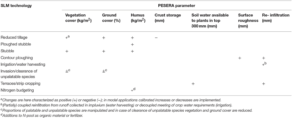
Table 2. Typical change in PESERA parameters and variables used to simulate mitigation options.

Reduced Tillage, Mulching, and/or Maintaining Ground Cover Vegetation within Tree Crops

It is common practice to clean-till between tree crops such as olives, almonds and vines after every significant rain to control competition for water from growing herbs and grasses (Fleskens and Stroosnijder, 2007; Xiloyannis et al., 2008). One alternative strategy consists of allowing some herb growth between trees, and controlling this growth through cutting or herbicide application. This may be associated with reduced or zero tillage. Another strategy is to mulch the surface with plant residues which may be pruned material from the trees or imported material. In PESERA tree crops are represented by a look-up table which specifies cover in each month of the year. Mulching can then be represented by editing this table (which already includes a pre-determined type for inter-sown or mulched tree crops) to increase cover in response to the chosen density of mulching (i.e., stubble in Table 2).

Retention of Crop Residues as Stubble at Harvesting of Arable and Other Crops

Vegetation biomass is set to zero and crop residues are normally assumed to be removed at every tillage, including at harvest. To represent the impact of leaving crop residues in the field, a proportion of the vegetation is transferred to the litter layer (stubble). The proportion removed must be at least the fraction of the crop taken to market (the harvest index). For grain crops this is normally in the range 30–50%, while for horticultural crops it may be much higher, up to 80% for green vegetables (i.e., all of the above-ground biomass). If additional mulch is brought in from outside, then the fraction returned to the organic soil may be larger. Since the crops grow according to the available soil moisture, the mulch fraction will also respond to the weather from year to year. In highly variable environments, it may be appropriate to set a target biomass (or implicitly yield), below which the crop is abandoned, and the entire biomass is plowed in as a mulch layer (plowed stubble in Table 2).

Reduced Tillage in Arable Crops

Minimum and zero tillage are represented in two ways. First, PESERA increases the rate of soil organic matter (SOM) decomposition by a factor of five in the month of tillage, representing the increased aeration of the soil that occurs. For minimum or zero tillage this ratio should be reduced or held to 1.0 (i.e., no increase in rate). Second, normal tillage events are assumed to reset to zero the vegetation biomass. Instead, tillage events around crop planting should have no effect on any pre-existing vegetation; and tillage associated with harvesting should remove the crop, and optionally the residues, but leave the small fraction (ca. 5%) of the biomass that represents the surviving non-crop plants. Crust storage is finally also reduced under minimum tillage (Table 2).

Irrigation and Water Harvesting for Croplands

An ideal irrigation system makes good the deficit between the water demand of the crop and the available precipitation. The simplest water harvesting system catches runoff from an area adjacent to the cropped field, and channels it to the cropped area, effectively increasing the water available to the crop during rainfall events and shortly afterwards. The difference between these extremes lies in the degree of buffering that allows collected water to be distributed according to crop demand rather than immediately during and after rainfall events. For pure irrigation, with unlimited supply, either from groundwater or reservoirs, the irrigation requirement on any day can be described by meeting a specified fraction of the crop demand, H:

$\begin{array}{ll}H=k\left(PE·WUE-r\right)& (4)\end{array}$

Where PE is the potential evapotranspiration, WUE is the water use efficiency (defined here as the dimensionless fraction of Potential ET required) of the crop at its current growth stage, r is the daily rainfall and k is the “irrigation fraction” (0 ≤ k ≤ 1).

For pure water harvesting from local sources, the water added to a cropped area can be described by the ratio, β, of bare (crusted) collecting area with a storage capacity h₀ to a cropped area with averaged storage capacity h_c. The total runoff, j, spread over the cropped area from a rainfall event of r can then be estimated as:

$\begin{array}{ll}j=\beta \left(r-h_0\right)+\left(r-h_c\right)& (5)\end{array}$

For intermediate systems, where water harvesting is used to fill a storage reservoir, the reservoir filling rate is given by the term β(r − h₀). Summing this over time, to determine the maximum irrigation fraction that can be supplied over the growing season we must solve:

$\begin{array}{ll}k=\frac{\sum \left[\beta \left(r-h_0\right)\right]}{\sum \left(PE·WUE-r\right)}& (6)\end{array}$

The cumulative difference between storage tank filling and use for irrigation determines the size of reservoir required and its reliability over a series of variable years.

Invasion and Clearance of Unpalatable Species

There is clear evidence of invasion of grazing lands by unpalatable species in southern Africa, e.g., in the DESIRE study site in Botswana, significantly reducing carrying capacities while apparently maintaining a relatively high biomass (Perkins et al., 2013). Overgrazing of fragile ecosystems has been a possible cause, although there is also some debate about the role of subtle climate changes. For a given average fraction of biomass α that is consumed, we here provisionally partition the calculated biomass between a proportion, p_U of unpalatable species and a proportion (1−p_U) of palatable species. The unpalatable proportion is then estimated as p_U = α∕α₀ for a parameter (to be determined) α₀ (necessarily >1), and the palatable portion is then consumed at the increased rate α/(1−α/α₀). This expression is valid for values of α < α₀/(1+α₀). This change reflects immediately on the carrying capacity of the land, although clearly an increase in unpalatable species tends, other things being equal, to provide some protection from erosion by both eater and wind, by increasing the land cover (Table 2).

This procedure allows the proportion of unpalatable shrubs to be estimated, but the process is not normally reversible, and unpalatable shrubs generally need to be removed by hand or machinery, sometimes repeatedly over a number of years.

Terracing and Strip Cropping

It is possible to represent patterns of terracing and strip cropping with a sub-grid model, explicitly representing the morphology and management patterns at a finer resolution within a single (1 km) grid cell. Here, we illustrate this approach for strip cropping and terracing across a uniform 100 m slope with 15 m elevation. In Figure 3, the area has been separated into equal strips with different land covers, represented here by different runoff thresholds of 30 and 90 mm, respectively. Curves show the calculated sediment transport (black dashed line) and the denudation (averaged from the top of the slope to the point in question) for every point on the slope, for a given average year of storms. Figure 3 shows that the denudation varies between limits of +2.4 and −3.6 mm. However, the average (0.51 mm) is very similar to that estimated for a uniformly covered slope with the average runoff threshold for the two types of strip (60 mm), which gives an average denudation of 0.48 mm. We are therefore modeling such strip-cropped areas with a runoff threshold that is the aerially weighted average of the land cover types within the cell.

FIGURE 3

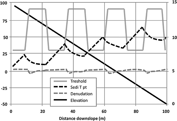
Figure 3. Sub-grid model for strip cropping on a 15% uniform slope. Right hand scale for elevation in meters. Left hand scale for other variables in mm. x-axis shows horizontal distance in meters.

Similarly, terracing has been simulated at the sub-grid scale (Figure 4). It can be seen that the terrace risers produce local peaks in erosion, but that the overall effect is almost identical to the erosion from a uniform slope, at the gradient of the terrace step, but with the weighted average runoff threshold (across tread and riser). This then provides the simple modeling rule that is used at the coarser grid scale of PESERA. It can also be seen that local erosion is concentrated on the tops of each riser, which should be reinforced and perhaps protected by diverting any pooled runoff away from the edge.

FIGURE 4

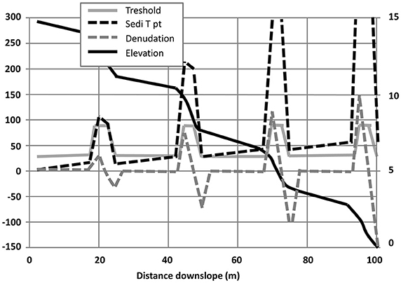
Figure 4. Sub-grid model of “hard” terraces, with 6% treads on an average 15% slope. Right hand scale for elevation in meters. Left hand scale for other variables in mm. x-axis shows horizontal distance in meters.

The effects on the effective modeled relief are more ambiguous for terracing. The lower gradients improve water retention in the lower part of the terrace treads, and this is accentuated by the re-deposition of any material eroded from above. Experiments suggest that the effective relief used in the grid cell should be reduced in the same proportion as the ratio of terrace tread gradient to overall average gradient. Over time, terraces generally accumulate deeper soils along their lower margins, often at the expense of the upper part of the terrace, and the deeper soils may help to retain more water for the growing crops (Table 2).

Nitrogen Budgeting and Rotations

The PESERA model already has a nitrogen cycling component, which was added for work on fertilizer application for upland UK environments. For simplicity, a single soil nitrogen store is simulated in the model. Nitrogen is added to the soil from litter-fall, fertilizer application, animal excretion, and a small amount in precipitation; and lost in runoff and to plants. Plants take up nitrogen from this store, and by direct atmospheric fixation, returning it to the soil store, and being removed to market. This component of the PESERA model then provides the response in biomass and yield to fertilizer application and nitrogen fixing crop rotations.

Evaluating Applicability Limitations of Strategies

An important step in PESERA-DESMICE is determining where each technology can, on biophysical grounds, in principle be applied. The purpose of this step is to rule out the area where technologies cannot be applied, such as constructing terraces on steep slopes with shallow soils. Factors considered include: soil depth, soil texture, slope gradient, landform, land use, climate, and distance to streams. Applicability limitations can be identified as minimum and/or maximum values, or as categories depending on the factor considered. Soil depth and texture limitations are, respectively, evaluated based on the PESERA “rootdepth” and “zm” input data layers. Slope gradient is calculated from a digital elevation model (DEM). Land use can be considered based on available land use maps for the study site of interest (as a minimum, the PESERA “use” data layer should be available which considers 12 land use types).

In the WOCAT methodology, landforms are defined based on two-dimensional position in the landscape and play an important role in defining application domains for SLM technologies. As landform maps are not common, in DESMICE, a simple landforms raster layer is calculated based on geomorphometric approaches (Evans, 1972), using a hydrologically corrected DEM as sole input. Table 3 shows the different landforms distinguished and criteria used to extract them from the DEM. First, streams, and ridges are extracted. Streams typically form a branched network one cell wide. Ridges are defined as any cell with convex profile curvature not receiving any flow from neighboring cells. Ridges generally form intermittent linear features indicative of (sub-) catchment boundaries but also occur as isolated cells of relative high position in the landscape. Plains and plateaus are subsequently identified as any area having a slope below 2%, and distinguished by an altitude threshold criterion. Areas tentatively classified as plains and plateaus are only maintained when their extension is larger than 1 km²; where this is not the case, they are classified as valley floors instead.

TABLE 3

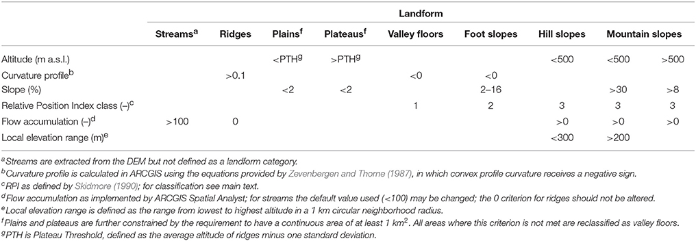
Table 3. Criteria used to extract a landforms map layer from a DEM.

The remaining landforms are identified drawing from a simple methodology developed by Skidmore (1990). The relative position index (RPI) of a cell in the landscape, defined as the Euclidean distance to the nearest streamline divided by the sum of Euclidean distances to the nearest streamline and ridge, was used to indicate three topographic positions: valleys (RPI = 0.15); footslopes (0.15 < RPI ≤ 0.6), and hillslopes (RPI > 0.6). Some adjustments were made to reclassify footslopes to hillslopes and vice-versa based on slope and curvature (c.f. Dragut and Blaschke, 2006; Saadat et al., 2008; Qin et al., 2009). Hillslopes and mountain slopes were likewise reclassified based on the Local Elevation Range (LER; Saadat et al., 2008) in a 1-km circular radius. A final step to arrive at a full and exclusive classification of each cell included (a) classifying cells with multiple classifications according to the following diminishing level of priority: ridges > plains > plateaus > valley floors > foot slopes > hill slopes > mountain slopes; and (b) expanding all categories at the expense of non-classified cells and reclassifying all areas consisting of < 5 connected cells to the landform in the majority of surrounding cells.

Table 4 shows some of the most commonly applied criteria to determine the applicability areas for various SLM technologies assessed within the DESIRE study sites.

TABLE 4

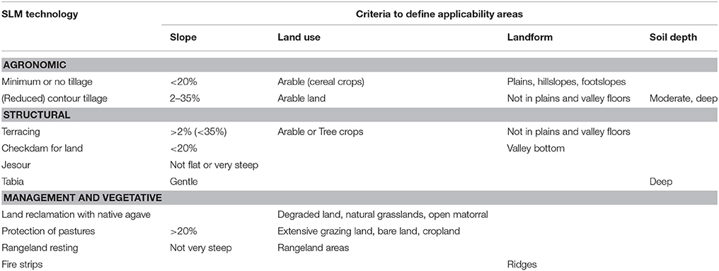
Table 4. Commonly used criteria to determine applicability areas for SLM technologies across DESIRE study sites.

Inventory Spatial Investment Cost Variation

If we ignore spatial variation, the investment cost of a technology (expressed in monetary units per hectare) is calculated in four phases:

1) Specifying the cost items required as inputs for the technology and the units in which they will be expressed;

2) Estimating what quantity of each cost item is required per hectare to implement the technology;

3) Determining a price per unit of each cost item;

4) Multiplying quantity and unit price of each cost item and summing to arrive at a total investment cost.

Methodologically calculating investment costs is straightforward, but knowing what quantities and prices to use can be complicated for many reasons, e.g., because the technology has not been widely implemented, or because it is usually implemented by individual farmers who have not recorded the quantities of inputs and costs. However, a major reason complicating the estimation of investment costs is that they are in fact variable. There is very likely not a single desertification mitigation technology which has a fixed investment cost. Hence, in attempting to establish a plausible cost estimate, often use is made of a frequent or average situation.

In DESMICE, a frequent or average quantity of a required input is called a base quantity. The model offers three modalities to vary required inputs spatially based on environmental factors: (i) no spatial variation applied; (ii) reclassification based on an input raster; or (iii) applying a formula. The result of this phase is thus a spatially-explicit quantity of each cost item required for implementing the technology.

The next phase is to calculate the spatially-explicit price of these inputs. DESMICE does this by calculating the transport cost from a market or source area to the technology implementation area. This includes specifying cost item source areas (or markets) by supplying an obligatory “source area type” (where the cost item can be obtained), an optional “input raster” if the source area type is an input raster to be reclassified or a fixed distance depending on reclassification of an input raster, and an obligatory “base price at source”. For the delineation of source areas, markets are assumed to be in towns. By default, transport costs will be determined using a Euclidian distance function. Per unit distance, a cost expressed in local currency units and time cost expressed in hours will be considered; the latter serves to reduce the effective length of working days by subtracting travel time. However, DESMICE offers a framework to calculate study-site specific transport costs in great detail, including consideration of different transport types, different cost algorithms, and use of an infrastructure layer taking into account the quality of road sections.

Spatially-Explicit Cost-Benefit Analysis

Investing in land degradation mitigation technologies should pay off through increased benefits and/or reduced costs relative to a situation without mitigation of land degradation. This means that not only are details needed about the investment and maintenance costs of technologies, but also about the production costs involved in the situations with and without mitigation. Apart from displaying spatially variable investment costs, SLM technologies may alter the production costs involved in the land use system in which they are applied. How this happens can be due to multiple mechanisms (see below). To take these effects into account, data on production costs are needed. These data are not included in the WOCAT QT database. Initially, it is thus required to put together an (informed) estimate for production costs in the case without applying the SLM technology.

i. A first way in which SLM technologies can alter production costs is by a change of production area. This may e.g., happen where structures occupy a part of the area under production in the case without mitigation.

ii. A second way in which production costs may be altered concerns management measures (or other types of measures implying a change of production system) affecting the fixed production costs. This includes for example introducing no-tillage systems (either as a management measure or as a change of management which could result from implementing narrow terraces rendering tractor access impossible).

iii. The third way in which production costs may be affected is when a technology involves a change of land use (e.g., technologies allowing extensive grazing land to be turned into arable production). Where this occurs, production costs associated with the new land use will be assumed to substitute the production costs without mitigation.

Spatial variability at the benefit-side is determined by the output from the PESERA model run. Here, variations in environmental conditions come into play. Similarly, as with spatial price variations due to distance to source areas and markets for inputs, DESMICE can consider distance functions to vary prices of outputs.

In investment analysis (i.e., for all SLM measures where implementation costs are expected to have a residual effect carrying over to the next year or longer), it is moreover important to understand the temporal streams of costs and benefits. As is commonly done in CBA, this assessment needs to take into account the opportunity cost of capital by introducing a discount factor. Hence, for each technology an economic lifetime needs to be specified, and for each study site a discount factor is required to make and compare financial cost-benefit analyses. Particularly the flow of benefits over time is often difficult to ascertain. The PESERA model can be run in time series mode to get insight into this. However, this is time consuming as it requires Monte Carlo type analyses. As an alternative, the outputs of model runs with and without mitigation can be considered as equilibrium situations, and a (linear) interpolation over a plausible time frame can offer an approximation. Fleskens (2012) illustrates how uncertainty about timing of effects can affect the financial viability of technologies.

Illustrative Model Applications

Input Data

PESERA requires monthly climate input layers as well as data layers describing land use, soil parameters, and relief (Kirkby et al., 2008). Depending on study sites, these input layers can differ in quality, with global data sources available as a back-up option. Model input data for each SLM technology primarily comes from the WOCAT database. Technologies documented in DESIRE and selected for PESERA-DESMICE application are compiled in Schwilch et al. (2012). The compiled documentation contains data from WOCAT QT questionnaires completed for each technology by the DESIRE study site teams based on expert opinion and experimental data. Additional data requests were made using two information sheets (for study sites and technologies, respectively). Furthermore, data from project field trials (Jetten and Shrestha, 2012) were used in parameterizing the DESMICE model. The ensuing illustrative applications are kept brief; more details about the cases is provided as Supplementary Material.

Minimum Tillage in Rainfed and Irrigated Maize, Cointzio (Mexico)

In six DESIRE study sites, various forms of minimum or reduced tillage were tested and modeled using PESERA-DESMICE. Here, we present results from one of these sites, the Cointzio watershed (640 km²), located in the altiplano of the Transmexican Volcanic Belt at an altitude of 1999–3007 m and receiving 750–1100 mm of rainfall annually (Supplementary Figure 1). Minimum tillage was considered here for both rainfed and irrigated maize crops. This was one of the few study sites for which a landforms map existed, allowing to assess the quality of the DESMICE landforms submodel output described in Section Evaluating Applicability Limitations of Strategies. In general terms, landforms coincided well, with major differences due to the survey-based map including landforms (volcanic cones, lava flows) not considered in the automated procedure and vice-versa ridges only considered in the latter (Figure 5).

FIGURE 5

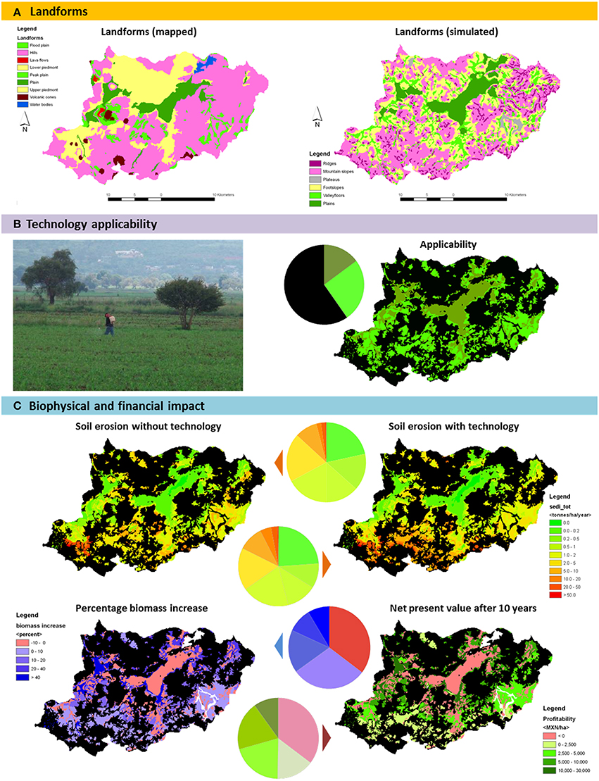
Figure 5. PESERA-DESMICE results for minimum tillage in rainfed and irrigated maize, Cointzio, Mexico. (A). Mapped and simulated landforms following geomorphometric approach; (B). Technology applicability is confined to arable lands whereby it is assumed that maize in plains (olive) is irrigated and maize on hillslopes and piedmonts (light green) rainfed; (C). Biophysical and financial impact: soil erosion with and without the technology, percentage biomass increase, and net present value after 10 years.

Production costs of maize were assumed to be the same under conventional and minimum tillage, but differentiated between hills and piedmonts (MXN 1000/ha [€59]) and plains (MXN 1700/ha [€100]), respectively. A harvest index of 0.4 is applied (i.e., 40% of crop biomass is marketable yield), and maize prices made variable in relation to zone: MXN 5/kg (€0.30) in hills and piedmonts and MXN 6/kg (€0.35) in plains. Minimum tillage was assumed to be possible on all arable land, with maize crop in plains assumed to be irrigated. The effect of reduced tillage on soil erosion was not very pronounced; however, a significant effect on rainfed yields (up to +50%) was simulated. On the other hand, a reduction of maize crops was simulated for irrigated areas. This might be due to increased competition for nutrients between maize and weeds. The economic viability calculations follow this pattern, whereby it could be noted that possible efficiency savings in production costs might improve viability. Based on these results, minimum tillage can be recommended for further (field) testing in rainfed areas.

Bench Terraces with Loess Soil Wall, Yanhe River Basin, China

Structural measures such as terraces were simulated for four study sites. A classic example is provided by bench terraces in the Yanhe River Basin (7678 km²), a tributary to the Yellow River originating from the Baiyu mountains on the Loess Plateau, China, covering an altitudinal range of 495–1795 m and experiencing precipitation between 420–530 mm per year (Supplementary Figure 2). The Loess Plateau is highly dissected, with mountain slopes constituting the dominant landform. Bench terraces are applicable on land under arable and tree crops on slopes higher than 2% (Figure 6). The modification of the slope gradient in PESERA results in great reduction of soil erosion rates, so that bench terraces are shown to hold the potential to completely control land degradation. This was also confirmed by field rainfall simulation experiments (Jetten and Shrestha, 2012).

FIGURE 6

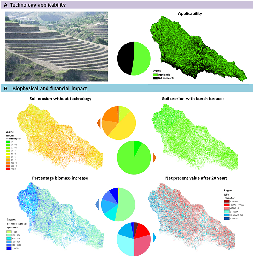
Figure 6. PESERA-DESMICE results for bench terraces with loess soil wall, Yanhe River Basin, China. (A) Technology applicability; (B). Biophysical and financial impact: soil erosion with and without the technology, percentage biomass increase, and net present value after 20 years.

Apple trees are grown on the resulting terraces. The change in land use from unproductive cereals to tree crops means that biomass increase is also spectacular. A harvest to total tree biomass index of 0.19 is used based on secondary data. The case without mitigation measures is assumed to be unproductive as cereal crops in the area are indicated to make a loss. An apple price of CNY 1.5/kg (€0.18) is used. A 10% discount rate and an economic life of 20 years were assumed, with apple trees starting to incrementally produce in year 4 (25%), 5 (50%), and 6 (75%), reaching full productivity from year 7. The cost of terracing ranges from CNY 80–35,392 (i.e., €10–4,358) for slopes ranging from 2–79%. The mean cost is CNY 10,864 ± 4901 (i.e., €1338 ± 603), to which tree planting costs of CNY 2052 (€253) still need to be added. Annual maintenance costs are set at 14.5% of initial investment costs and production costs for apple production (chemical inputs and labor) are CNY 9664 (€1190).

With these assumptions, bench terracing is profitable in slightly less than half of the applicable area. The western part of the study area (more productive) and the less steep slopes are the most viable areas. Despite the profitability, the fact that the payback period for the investment is long (close to 20 years) might deter land users from applying the technology, a message also conveyed from stakeholder evaluation workshops (Stringer et al., 2014). PESERA-DESMICE model results are sensitive to changes in the spatial variability of investment costs, with both the extent and distribution across the landscape of financial viability altering significantly (Fleskens, 2012). Expert opinion on the impact of bench terraces is provided in Supplementary Figure 3.

Primary Strip Network System for Fuel Management, Mação, Portugal

The Primary Strip Network for Fuel Management (PSNSFM) is a municipal plan to control forest fires in Mação, a municipality located on the northern bank of the lower Tejo River in Central Portugal (Supplementary Figure 4). The area covers 400 km², ranges from 28–640 m above sea level and experiences a South-North rainfall gradient of < 600–1000 mm. The PSNSFM follows many ridges in the landscape. In total, 1287 ha of strips are included in the plan. Strips are assumed to be 100% effective as fire break when maintained to reduce fuel load every 2 years. The initial investment costs are €1,741,358; thereafter, maintenance costs of €1,158,454 are assumed to be made biannually. These costs are based on a cost estimate for clearing costs of €73 per ton biomass. A discount rate of 10% is applied and a lifetime of 10 years has been set, with assessment of benefits derived from analysis of avoidable damage from observed fire-affected areas over the period 2001–2009. A simplified representation of fire in PESERA was used as wind speed data was not available. Instead of a FDI score, this approach yielded a Fire Severity Index (FSI) score, solely based on relative humidity and amount of combustible biomass. Figure 7 clearly shows the reduced FSI values simulated for the situation 2 years after establishment of the strip network (FSI values outside the strip network are not affected).

FIGURE 7

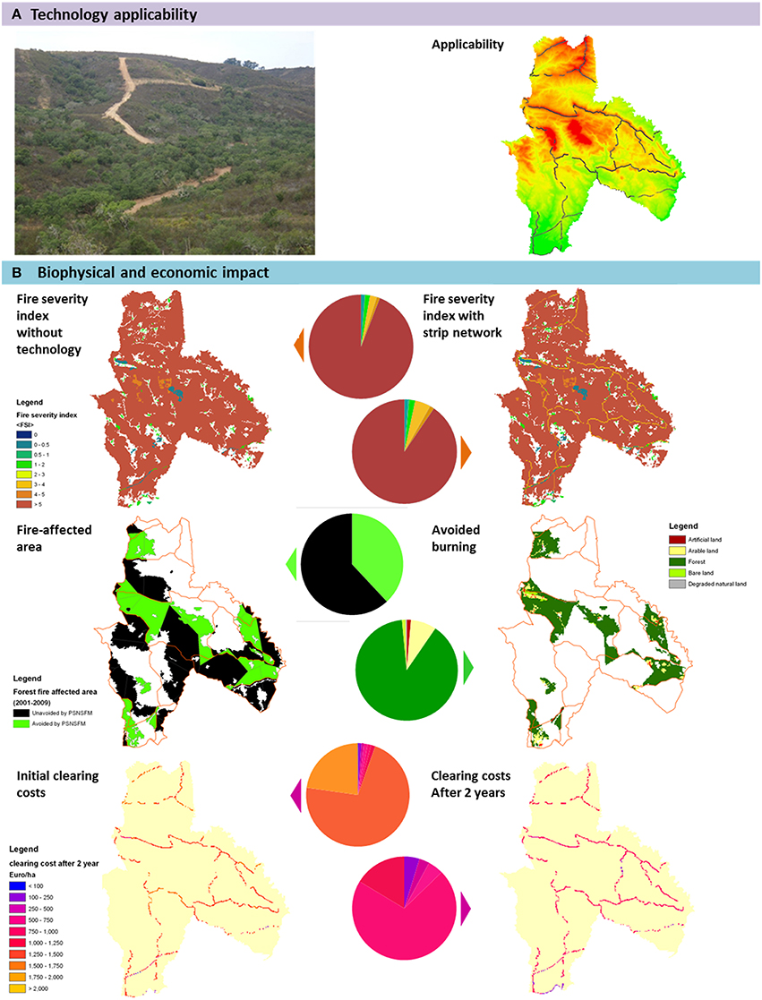
Figure 7. PESERA-DESMICE results for Primary Strip Network System for Fuel Management, Mação, Portugal. (A). Technology applicability: municipal strip network plan of 1287 ha; (B). Biophysical and economic impact: fire severity index with and without the strip network, fire-affected area and avoidable burning, initial and biannual clearing cost.

Forest fires that would have been prevented if the PSNSFM were in place are substantial, averaging 958 ha annually. Based on fire damage costs differentiated according to the land use of burnt areas (values between €100/ha for degraded land and €100,000/ha for built-up land, with damage to forest itself assessed at €2000/ha), avoided damage is €3,085,400 annually. Although this analysis does not consider fire extinguishing and replanting costs, the PSNSFM appears to be very viable (NPV of over €14 million). Results are however heavily influenced by the catastrophic 2003 forest fires which were responsible for more than three-quarters of the total damage between 2001 and 2009. Fleskens et al. (2012) show that not planning for events of this unprecedented magnitude would render the PSNSFM uneconomic. Supplementary Figure 5 displays impacts of the PSNSFM as recorded in experiments and elicited from experts and local stakeholders.

Discussion

As explained and illustrated above, the PESERA-DESMICE framework allows grid-based assessment of spatial variability of biophysical impact and economic viability of land degradation mitigation technologies. It thereby considers both spatial variability in costs and effectiveness. This adds an additional variable in terms of variable implementation/establishment cost compared to similar assessments documented in the literature, e.g., by Heckbert et al. (2012) for prescribed fire and Evans et al. (2015) for assisted natural regeneration. These studies differ in how they deal with opportunity costs: whereas Heckbert et al. (2012) assume interventions in unmanaged landscapes have no opportunity costs, Evans et al. (2015) consider reforestation on farmed land. Our approach accommodates both types of assessment approaches, in principle from the land manager's perspective, although this can be scaled up to a landscape scale assessment from a societal perspective. In Heckbert et al.'s assessment, prescribed fire was deemed viable across a large area in Northern Australia but relied on a carbon payment. In our Portuguese case study actual avoided damage was the sole benefit considered. Birch et al. (2010) considered multiple ecosystem services in their assessment of cost-effectiveness of dryland restoration and reported largely negative NPV in case of active restoration efforts. It is clear that such assessments are highly context-specific, and their findings cannot easily be generalized or compared.

The specific remediation options modeled in the case studies were scaled up from small-scale experiments and modeling results are therefore inherently difficult to validate. Spatial sampling as e.g., performed by Forouzangohar et al. (2014) could be helpful to validate some model outputs (e.g., biomass production) but is far less straightforward when considering soil conservation. Our approach to validation has therefore relied on stakeholder and expert opinion. Land degradation in the case without mitigation measures was found to coincide to different degree with expert mapping, e.g., agreement was quite high in China but limited in Mexico (Fleskens et al., 2014). Stakeholder opinion about effectiveness and viability of technologies was generally in line with PESERA-DESMICE results (Stringer et al., 2014). A reason for this better agreement about technologies than baseline results could be that the technology results can also be regarded in relative terms, whereas local experts' mapping of land degradation is context-specific and therefore likely not uniform across different study sites. Another approach could be to compare different modeling approaches across a range of conditions to bring out areas where there is agreement and divergence (e.g., Bagstad et al., 2013).

Panagos et al. (2015a), in a continental-scale high resolution model assessment of soil erosion, conclude that soil conservation practices have reduced soil loss in the past decade by 20% on arable land and 9.5% overall in Europe. They too stress the value of spatial maps in pointing to hotspots where the highest soil loss reduction potential can be realized, and in determining the economic value of such measures, and the policies that create financial incentives for their adoption. The current applicability of reduced and no tillage practices are shown to cover large areas (over 25% of agricultural lands in the EU); however, stone walls and grass margins have the most important impact on soil loss rates where they are applied locally (Panagos et al., 2015b). A combination of different remediation options may be required to achieve environmental conservation targets (e.g., Schmidt and Zemadim, 2015). The PESERA-DESMICE framework can be helpful in this context to indicate the most effective measures in each location.

Our methodological framework as here presented allows not only to predict the biophysical impact of management practices, but also to assess the spatially-explicit financial viability of doing so. Such information has been shown to be important, particularly in designing cost-effective policies for conservation benefits (c.f. Naidoo et al., 2006). The direct consideration of cost-effectiveness in the modeling framework, and its suitability for scenario analysis render it a useful tool for regional stakeholder engagement. Our first evaluation of the value of this type of scenario modeling has been quite positive (Stringer et al., 2014), but requires more in-depth future assessment. Lessons from similar approaches elsewhere also point to limitations, and the need to implement strategies to overcome these (e.g., Meyer et al., 2015). Through involving stakeholders from the start, and actively engage them in verifying and using model outputs, the approach taken has contributed to social learning in terms of knowledge exchange and improved knowledge of modeled insights (Stringer et al., 2014).

Whereas PESERA-DESMICE currently simulates biomass production and selected regulation services, the approach could be easily extended to cover a wider portfolio of ecosystem services. The grid-based nature of the model can be further exploited to develop cell interactions (as e.g., explained for the fire module, or routing of run-off and sediments). The framework as here described deals particularly with common processes of land degradation in drylands (water and wind erosion, overgrazing, wildfires). Other degradation processes could also be added to the framework.

Conclusions

The PESERA-DESMICE modeling framework offers a sophisticated analytical tool to assess the biophysical effects and financial viability of land degradation mitigation technologies. The framework overcomes a number of challenges to incorporate inputs from multiple stakeholders in very different contexts into the modeling process, in order to enhance both the realism and relevance of outputs for policy and practice. The spatially-explicit CBA is able to demonstrate where minimum conditions for land users to adopt SLM measures are met, enabling targeting and anticipation of adoption processes across landscapes and assessment of their consequent environmental effects. Although, PESERA-DESMICE does show interesting results when run with generally available data and generic cost estimates of technologies, assessment could be improved by better quality input data. Such better quality data is not trivial where modeling is employed to understand the impact of subtle drivers such as deteriorating land quality and climate change. The temporal dimension of changes in productivity is crucial for land users. Better disentangling the immediate and gradual aspects of biophysical changes can improve the accuracy of the assessment. Nonetheless, the illustrations of the PESERA-DESMICE framework yielded important messages for environmental managers, such as where to test technologies in the field, how to stimulate adoption of SLM, and most importantly spatial targeting of SLM technologies. Embedding the modeling in a participatory assessment process enabled qualitative validation of results and contributed to social learning.

Author Contributions

LF designed the PESERA-DESMICE modeling framework with contributions from MK and BI. MK and BI developed the PESERA model and its extensions. LF developed the DESMICE model. BI and LF applied the modeling framework to case studies. LF wrote the paper with contributions from BI and MK.

Conflict of Interest Statement

The authors declare that the research was conducted in the absence of any commercial or financial relationships that could be construed as a potential conflict of interest.

Acknowledgments

We thank the DESIRE study site teams in China, Mexico, and Portugal, in particular Christian Prat, Wang Fei, Sandra Valente, and João Soares for providing case study data.This study was funded by the EU Framework 6 Desertification Mitigation & Remediation of Land—a Global Approach for Local Solutions (DESIRE) Project (037046). Helpful comments from the two reviewers are gratefully acknowledged.

Supplementary Material

The Supplementary Material for this article can be found online at: https://www.frontiersin.org/article/10.3389/fenvs.2016.00031

Footnotes

1. ^WOCAT stands for World Overview of Conservation Approaches and Technologies, which is simultaneously a network, system for documenting, and database of sustainable land management information. WOCAT is the database of choice for the UNCCD (http://www.wocat.net).

References

Bagstad, K. J., Semmens, D. J., and Winthrop, R. (2013). Comparing approaches to spatially explicit ecosystem service modeling: a case study from the San Pedro River, Arizona. Ecosyst. Serv. 5, 40–50. doi: 10.1016/j.ecoser.2013.07.007

CrossRef Full Text | Google Scholar

Birch, J. C., Newton, A. C., Aquino, C. A., Cantarello, E., Echeverría, C., Kitzberger, T., et al. (2010). Cost-effectiveness of dryland forest restoration evaluated by spatial analysis of ecosystem services. Proc. Natl. Acad. Sci. U.S.A. 107, 21925–21930. doi: 10.1073/pnas.1003369107

PubMed Abstract | CrossRef Full Text | Google Scholar

Borrelli, P., Panagos, P., Ballabio, C., Lugato, E., Weynants, M., and Montanarella, L. (2014). Towards a Pan-European assessment of land susceptibility to wind erosion. Land Degrad. Develop. doi: 10.1002/ldr.2318. [Epub ahead of print].

CrossRef Full Text | Google Scholar

Camm, J. D., Polasky, S., Solow, A., and Csuti, B. (1996). A note on optimal algorithms for reserve site selection. Biol. Cons. 78, 353–355. doi: 10.1016/0006-3207(95)00132-8

CrossRef Full Text

Crossman, N. D., Perry, L. M., Bryan, B. A., and Ostendorf, B. (2007). CREDOS: a conservation reserve evaluation and design optimisation system. Environ. Mod. Softw. 22, 449–463. doi: 10.1016/j.envsoft.2005.12.006

CrossRef Full Text | Google Scholar

de Graaff, J. (1996). The Price of Soil Erosion – An Economic Evaluation of Soil Conservation and Watershed Development. Ph.D. thesis, Wageningen University, Netherlands.

Dragut, L., and Blaschke, T. (2006). Automated classification of landform elements using object-based image analysis. Geomorphology 81, 330–344. doi: 10.1016/j.geomorph.2006.04.013

CrossRef Full Text | Google Scholar

Esteves, T. C. J., Kirkby, M. J., Shakesby, R. A., Ferreira, A. J. D., Soares, J. A. A., Irvine, B. J., et al. (2012). Mitigating land degradation caused by wildfire: application of the PESERA model to fire-affected sites in central Portugal. Geoderma 191, 40–50. doi: 10.1016/j.geoderma.2012.01.001

CrossRef Full Text | Google Scholar

Evans, I. S. (1972). “General geomorphometry, derivatives of altitude and descriptive statistics,” in Spatial Analysis in Geomorphology, ed R. J. Chorley (London: Methuen). 17–90.

Evans, M. C., Carwardine, J., Fensham, R. J., Butler, D. W., Wilson, K. A., Possingham, H. P., et al. (2015). Carbon farming via assisted natural regeneration as a cost-effective mechanism for restoring biodiversity in agricultural landscapes. Environ. Sci. Pol. 50, 114–129. doi: 10.1016/j.envsci.2015.02.003

CrossRef Full Text | Google Scholar

Fleskens, L. (2012). Modelling the impact and viability of sustainable land management technologies: what are the bottlenecks? Agro. Environ. Available online at: http://library.wur.nl/ojs/index.php/AE2012/article/download/12411/12607

Fleskens, L., Ataev, A., Mamedov, B., and Spaan, W. P. (2007). Desert water harvesting from takyr surfaces: assessing the potential of traditional and experimental technologies in the Karakum. Land Deg. Dev. 18, 17–39. doi: 10.1002/ldr.759

CrossRef Full Text | Google Scholar

Fleskens, L., Irvine, B., Kirkby, M. J., and Nainggolan, D. (2012). Model Outputs for Each Hotspot Site to Identify the Likely Environmental, Environmental and Social Effects of Proposed Remediation Strategies. DESIRE Report 100 D5.3.1 April2012.

Fleskens, L., Nainggolan, D., and Stringer, L. C. (2014). An exploration of scenarios to support sustainable land management using the PESERA-DESMICE integrated environmental socio-economic models. Environ. Manage. 54, 1005–1021. doi: 10.1007/s00267-013-0202-x

PubMed Abstract | CrossRef Full Text | Google Scholar

Fleskens, L., and Stroosnijder, L. (2007). Is soil erosion in olive groves as bad as often claimed? Geoderma 141, 260–271. doi: 10.1016/j.geoderma.2007.06.009

CrossRef Full Text | Google Scholar

Fleskens, L., Stroosnijder, L., Ouessar, M., and de Graaff, J. (2005). Evaluation of the on-site impact of water harvesting in southern Tunisia. J. Arid Environ. 62, 613–630. doi: 10.1016/j.jaridenv.2005.01.013

CrossRef Full Text | Google Scholar

Forouzangohar, M., Crossman, N. D., MacEwan, R. J., Wallace, D. D., and Bennett, L. T. (2014). Ecosystem services in agricultural landscapes: a spatially explicit approach to support sustainable soil management. Sci. World J., 2014:483298. doi: 10.1155/2014/483298

PubMed Abstract | CrossRef Full Text | Google Scholar

Gang, C., Zhou, W., Chen, Y., Wang, Z., Sun, Z., Li, J., et al. (2014). Quantitative assessment of the contributions of climate change and human activities on global grassland degradation. Environ. Earth Sci. 72, 4273–4282. doi: 10.1007/s12665-014-3322-6

CrossRef Full Text | Google Scholar

Heckbert, S., Russell-Smith, J., Reeson, A., Davies, J., James, G., and Meyer, C. (2012). Spatially explicit benefit–cost analysis of fire management for greenhouse gas abatement. Austral Ecol. 37, 724–732. doi: 10.1111/j.1442-9993.2012.02408.x

CrossRef Full Text | Google Scholar

Hessel, R., Reed, M. S., Geeson, N., Ritsema, C. J., van Lynden, G., Karavitis, C. A., et al. (2014). From framework to action: the DESIRE approach to combat desertification. Environ. Manage. 54, 935–950. doi: 10.1007/s00267-014-0346-3

PubMed Abstract | CrossRef Full Text | Google Scholar

Hilker, T., Natsagdorj, E., Waring, R. H., Lyapustin, A., and Wang, Y. (2014). Satellite observed widespread decline in Mongolian grasslands largely due to overgrazing. Glob. Change Biol. 20, 418–428. doi: 10.1111/gcb.12365

PubMed Abstract | CrossRef Full Text | Google Scholar

Jetten, V., and Shrestha, D. (eds). (2012). Implementation of Conservation Technologies at Stakeholder Level. Results of Field Experiments. DESIRE Report 91 D4.3.1 April2012.

Kenney, P. M., Keith, T. G., Ng, T. T., and Linn, R. R. (2008). In-field determination of drag through grass for a forest-fire simulation model. WIT Trans. Ecol. Environ. 119, 23–29. doi: 10.2495/FIVA080031

CrossRef Full Text | Google Scholar

Khabarov, N., Krasovskii, A., Obersteiner, M., Swart, R., Dosio, A., San-Miguel-Ayanz, J., et al. (2016). Forest fires and adaptation options in Europe. Reg. Environ. Change 16, 21–30. doi: 10.1007/s10113-014-0621-0

CrossRef Full Text | Google Scholar

King, J., Nickling, W. G., and Gillies, J. A. (2008). Investigations of the law-of-the-wall over sparse roughness elements. J. Geophys. Res. Earth Surf. 113. doi: 10.1029/2007jf000804

CrossRef Full Text | Google Scholar

Kirkby, M., Irvine, B., Poesen, J., Borselli, L., and Reed, M. (2010). Improved Process Descriptions Integrated Within the PESERA Model in Order to be Able to Evaluate the Effects of Potential Prevention and Remediation Measures. DESIRE Report 75 D5.2.1 March2010.

Kirkby, M. J., Irvine, B. J., Jones, R. J. A., Govers, G., Boer, M., Cerdan, O., et al. (2008). The PESERA coarse scale erosion model for Europe. I. – model rationale and implementation. Eur. J. Soil. Sci. 59, 1293–1306. doi: 10.1111/j.1365-2389.2008.01072.x

CrossRef Full Text | Google Scholar

Kuhlman, T., Reinhard, S., and Gaaff, A. (2010). Estimating the costs and benefits of soil conservation in Europe. Land Use Pol. 27, 22–32. doi: 10.1016/j.landusepol.2008.08.002

CrossRef Full Text | Google Scholar

Liniger, H. P., and Critchley, W. (eds). (2007). Where the Land is Greener – Case Studies and Analysis of Soil and Water Conservation Initiatives Worldwide. Berne: CTA/FAO/UNEP/CDE.

Google Scholar

Ludi, E. (2004). Economic Analysis of Soil Conservation: Case Studies from the Highlands of Amhara Region, Ethiopia. African Studies Series A 18. Berne: University of Berne.

Google Scholar

Meyer, W. S., Bryan, B. A., Summers, D. M., Lyle, G., Wells, S., McLean, J., et al. (2015). Regional engagement and spatial modelling for natural resource management planning. Sustain. Sci. doi: 10.1007/s11625-015-0341-5. [Epub ahead of print].

CrossRef Full Text | Google Scholar

Montanarella, L., Pennock, D. J., McKenzie, N., Badraoui, M., Chude, V., Baptista, I., et al. (2016). World's soils are under threat. SOIL 2, 79–82. doi: 10.5194/soil-2-79-2016

CrossRef Full Text

Naidoo, R., Balmford, A., Ferraro, P. J., Polasky, S., Ricketts, T. H., and Rouget, M. (2006). Integrating economic costs into conservation planning. Trends Ecol. Evol. 21, 682–687. doi: 10.1016/j.tree.2006.10.003

PubMed Abstract | CrossRef Full Text | Google Scholar

NASA, (2013). Available online at: http://thunder.nsstc.nasa.gov/index.html

National Research Council (2000). Nutrient Requirements of Beef Cattle. Washington, DC: National Academy Press.

Ninan, K. N., and Lakshmikanthamma, S. (2001). Social cost-benefit analysis of a watershed development project in Karnataka, India. Ambio 30, 157–161. doi: 10.1579/0044-7447-30.3.157

PubMed Abstract | CrossRef Full Text | Google Scholar

Panagos, P., Borrelli, P., Meusburger, K., van der Zanden, E. H., Poesen, J., and Alewell, C. (2015b). Modelling the effect of support practices (P-factor) on the reduction of soil erosion by water at European Scale. Environ. Sci. Pol. 51, 23–34. doi: 10.1016/j.envsci.2015.03.012

CrossRef Full Text | Google Scholar

Panagos, P., Borrelli, P., Poesen, J., Ballabio, C., Lugato, E., Meusburger, K., et al. (2015a). The new assessment of soil loss by water erosion in Europe. Environ. Sci. Pol. 54, 438–447. doi: 10.1016/j.envsci.2015.08.012

CrossRef Full Text | Google Scholar

Pausas, J. G., Llovet, J., Rodrigo, A., and Vallejo, R. (2008). Are wildfires a disaster in the Mediterranean basin? – a review. Int. J. Wildland Fire 17, 713–723. doi: 10.1071/WF07151

CrossRef Full Text | Google Scholar

Perkins, J. S., Reed, M. S., Akanyang, L., Atlhopheng, J. R., Chanda, R., Magole, L., et al. (2013). Making land management more sustainable: experience implementing a new methodological framework in Botswana. Land Deg. Dev. 24, 463–477. doi: 10.1002/ldr.1142

CrossRef Full Text | Google Scholar

Pimentel, D., Harvey, C., Resosudarmo, P., Sinclair, K., Kurz, D., McNair, M., et al. (1995). Environmental and economic costs of soil erosion and conservation benefits. Science 267, 1117–1123. doi: 10.1126/science.267.5201.1117

PubMed Abstract | CrossRef Full Text | Google Scholar

Posthumus, H., and de Graaff, J. (2005). Cost-benefit analysis of bench terraces, a case study in Peru. Land Deg. Dev. 16, 1–11. doi: 10.1002/ldr.637

CrossRef Full Text | Google Scholar

Qin, C. Z., Zhu, A. X., Shi, X., Li, B. L., Pei, T., and Zhou, C. H. (2009). Quantification of spatial gradation of slope positions. Geomorphology 110, 152–161. doi: 10.1016/j.geomorph.2009.04.003

CrossRef Full Text | Google Scholar

Reed, M. S., Buenemann, M., Atlhopheng, J., Akhtar-Schuster, M., Bachmann, F., Bastin, G., et al. (2011). Cross-scale monitoring and assessment of land degradation and sustainable land management: a methodological framework for knowledge management. Land Deg. Dev. 22, 261–271. doi: 10.1002/ldr.1087

CrossRef Full Text | Google Scholar

Saadat, H., Bonnell, R., Sharifi, F., Mehuys, G., Namdar, M., and Ale-Ebrahimet, S. (2008). Landform classification from a digital elevation model and satellite imagery. Geomorphology 100, 453–464. doi: 10.1016/j.geomorph.2008.01.011

CrossRef Full Text | Google Scholar

Schmidt, E., and Zemadim, B. (2015). Expanding sustainable land management in Ethiopia: scenarios for improved agricultural water management in the Blue Nile. Agric. Water Manage. 158, 166–178. doi: 10.1016/j.agwat.2015.05.001

CrossRef Full Text | Google Scholar

Schmuck, G., San-Miguel-Ayanz, J., Durrant, T., Boca, R., Libertà, G., Petroliagkis, T., et al. (2015). Forest Fires in Europe, Middle East and North Africa 2014. EUR 27400 EN. Luxembourg: Publications Office of the European Union.

Google Scholar

Schwilch, G., Bachmann, F., and Liniger, H. P. (2009). Appraising and selecting conservation measures to mitigate desertification and land degradation based on stakeholder participation and global best practices. Land Deg. Dev. 8, 308–326. doi: 10.1002/ldr.920

CrossRef Full Text | Google Scholar

Schwilch, G., Hessel, R., and Verzandvoort, S. (eds). (2012). Desire for Greener Land. Options for sustainable land management in drylands. Bern: University of Bern-CDE/Alterra/ISRIC/CTA.

Skidmore, A. K. (1990). Terrain position as mapped from a gridded digital elevation model. Int. J. Geogr. Inf. Sci. 4, 33–49. doi: 10.1080/02693799008941527

CrossRef Full Text

Stolte, J., Tesfai, M., Øygarden, L., Kværnø, S., Keizer, J., Verheijen, F., et al. (2015). Soil Threats in Europe. EUR 27607 EN. Luxembourg: Publications Office of the European Union.

Google Scholar

Stringer, L. C., Fleskens, L., Reed, M. S., de Vente, J., and Zengin, M. (2014). Participatory evaluation of monitoring and modelling of sustainable land management technologies in areas prone to land degradation. Environ. Manage. 54, 1022–1042. doi: 10.1007/s00267-013-0126-5

PubMed Abstract | CrossRef Full Text | Google Scholar

Tulloch, A. I. T., Tulloch, J. V. D., Evans, M. C., and Mills, M. (2014). The value of using feasibility models in systematic conservation planning to predict landholder management uptake. Cons. Biol. 28, 1462–1473. doi: 10.1111/cobi.12403

PubMed Abstract | CrossRef Full Text | Google Scholar

Turner, K. G., Anderson, S., Gonzales-Chang, M., Costanza, R., Courville, S., Dalgaard, T., et al. (2016). A review of methods, data, and models to assess changes in the value of ecosystem services from land degradation and restoration. Ecol. Mod. 390, 190–207. doi: 10.1016/j.ecolmodel.2015.07.017

CrossRef Full Text | Google Scholar

UNCCD (1994). United Nations Convention to Combat Desertification in Countries Experiencing Serious Drought and/or Desertification, Particularly in Africa. Document A/AC. 241/27, 12. 09. 1994 with Annexes. New York, NY: United Nations.

Venevsky, S., Thonicke, K., Sitch, S., and Kramer, W. (2002). Simulating fire regimes in human-dominated ecosystems: Iberian case study. Glob. Change Biol. 8, 984–998. doi: 10.1046/j.1365-2486.2002.00528.x

CrossRef Full Text | Google Scholar

Visser, S. M., and Sterk, G. (2007). Nutrient dynamics—wind and water erosion at the village scale in the Sahel. Land Degrad. Dev. 18, 578–588. doi: 10.1002/ldr.800

CrossRef Full Text | Google Scholar

Xiloyannis, C., Martinez Raya, A., Kosmas, C., and Favia, M. (2008). Semi-intensive olive orchards on sloping land: requiring good land husbandry for future development. J. Environ. Manage. 89, 110–119. doi: 10.1016/j.jenvman.2007.04.023

PubMed Abstract | CrossRef Full Text | Google Scholar

Zevenbergen, L. W., and Thorne, C. R. (1987). Quantitative analysis of land surface topography. Earth Surf. Proc. Land 12, 47–56. doi: 10.1002/esp.3290120107

CrossRef Full Text | Google Scholar