Site Characteristics Mediate the Relationship Between Forest Productivity and Satellite Measured Solar Induced Fluorescence

Introduction

Gross Primary Production (GPP), which is a measure of the flux of carbon taken up by vegetation through photosynthesis, is the largest components (along with ecosystem respiration) of CO₂ exchange between terrestrial ecosystems and the atmosphere. Solar-Induced Chlorophyll Fluorescence (SIF) has been gaining popularity as a tool to estimate GPP indirectly. SIF data can be obtained through either tower- or airborne-based measurements (Chang et al., 2020) and satellite remote sensing instruments (Frankenberg et al., 2011), where the latter presents a promising alternative for accurate global GPP modeling.

Solar-Induced Chlorophyll Fluorescence represents a small fraction of the Photosynthetically Active Radiation (PAR) that is absorbed by chlorophyll pigments and re-emitted as a faint glow mainly in the range of 650–800 nm (Papageorgiou, 1975; Baker, 2008). Since both light reaction of photosynthesis and SIF compete for the same excitation energy, SIF can be an indicator of the functioning of the photosynthetic mechanism (Porcar-Castell et al., 2014). Conceptually, both GPP and SIF are considered to be proportional to Absorbed PAR (APAR; Monteith, 1972; Guanter et al., 2014). Non-Photochemical Quenching (NPQ), a process for excess energy dissipation (Jonard et al., 2020), is a third pathway for light use, potentially playing a major role in the GPP:SIF relations (Wohlfahrt et al., 2018).

Based on the information provided by SIF on the actual electron transport from Photosystem II to Photosystem I, Gu et al. (2019) derived fundamental equations linking SIF to C₃ and C₄ photosynthesis at the canopy level using a big leaf approach, thus bridging leaf scale and canopy scales for GPP:SIF. However, many canopy-level quantities used in the derivation could not be estimated through remote sensing approaches or flux measurements, which limits the wide use of this formulation. Nevertheless, it is a benchmark for investigating GPP:SIF at larger spatial timescales.

Solar-Induced Chlorophyll Fluorescence is reported to be linearly related to GPP at the diurnal and seasonal scales in various studies across a variety of sites (Joiner et al., 2014; Yang et al., 2015; Zhang et al., 2016b; Yang H. et al., 2017; Du et al., 2019; Magney et al., 2019; He et al., 2020b; Qiu et al., 2020). However, the slopes of these linear GPP:SIF relations differ across sites, biomes, and vegetation types (Smith et al., 2018; Sun et al., 2018; Zhang et al., 2018b). SIF is shown to be a relevant indicator of crop productivity (Guanter et al., 2014; Guan et al., 2016, 2017; Zhang et al., 2018a; He et al., 2020a) and seasonal phenology (Joiner et al., 2014; Jeong et al., 2017; Yang H. et al., 2017). However, at instantaneous to hourly temporal scales, the GPP:SIF correlation is not as strong as at longer timescales, i.e., from days to seasons and years (Zhang et al., 2018c; Marrs et al., 2020). Observations and models at short timescales are needed to characterize the environmental effects that cause rapid variations (i.e., intra-daily, and inter-daily within season) of GPP, such as light saturation and water stress.

At sub-diurnal or half-hourly timescales, GPP:SIF was reported to follow an asymptotic trend (Li et al., 2018a; Chen et al., 2020). Indeed, GPP saturates at high APAR, while SIF keeps increasing as APAR increases, leading to a hyperbolic relationship between SIF and GPP at the instantaneous timescale (Damm et al., 2015; Gu et al., 2019). This hyperbolic-shaped relationship is less apparent over longer timescales, when variability in SIF and GPP is dominated seasonal variations in canopy structure, as estimated with the Leaf Area Index (LAI), whose effects are present in both SIF and GPP signals (Lu et al., 2018; Balzarolo et al., 2019; Dechant et al., 2020). Thus, the GPP:SIF correlation becomes more linear and relatively less sensitive to faster variations in the environmental drivers and plant physiological stress. Beyond physiological effects that govern GPP:SIF at the leaf level, non-linear relationships of GPP:SIF at the flux-footprint scale can therefore also be attributed to canopy structure. In addition, SIF is function of the view geometry. SIF is emitted from leaves exposed to sunlight, thus all conditions involved in the interaction between leaves, incident radiation, and view angle are important drivers of SIF observed signal. Therefore, canopy structure, and specifically gap fraction, leaf angle, and clumping index, and their interactions with the incident radiation angle, and the satellite viewing angle are important factors influencing GPP:SIF (Dechant et al., 2020).

The ambiguity in the GPP:SIF relations across timescales opens the door for further investigations of the effects of short-term environmental variables on this correlation, notably water stress. Beside variations in vegetation structure, GPP can be modulated by both non-stomatal and stomatal regulation. In periods of water shortage or stress, indicated by high vapor pressure deficit (VPD) and low soil moisture (Zhou et al., 2019), stomata tend to close in order to reduce water loss through transpiration, simultaneously resulting in a decrease in photosynthetic rate. However, the extent of stomatal response to water stress is species specific (Matheny et al., 2015; Konings and Gentine, 2017). Furthermore, reductions in stomatal conductance under high VPD do not necessarily translate into a reduction in photosynthesis of the same magnitude due to variations in intrinsic water use efficiency (Zhang et al., 2019; Green et al., 2020; Grossiord et al., 2020). Non-stomatal limitation of photosynthesis can be induced by water-stress through xylem cavitation, decrease in mesophyll conductance for CO₂ (Flexas et al., 2016), and reduction in metabolic efficiency of the enzyme Rubisco (Grassi and Magnani, 2005).

The partitioning of APAR between GPP, NPQ, and SIF is sensitive to environmental conditions, such as incoming PAR, canopy structure (as represented by the fraction of the absorbed PAR, which depends mainly on LAI, but also other structural characteristics of the canopy, such as gap fraction, leaf clustering, and leaf angles), and soil water availability. At low light, most of the absorbed PAR is utilized for photosynthesis, thus increasing its efficiency. However, at high light, energy-consuming biochemical reactions of CO₂ assimilation and electron transport chain saturate, leading to a re-allocation of excess energy into SIF and NPQ (Porcar-Castell et al., 2014), thus modifying the partitioning between SIF and GPP. Such light saturation or water stress scenarios should lead to deviation from a linear relationship between GPP and SIF.

Differences in SIF responses can also stem from SIF measurement methods, which can be either active, i.e., ground-based through pulse amplitude-modulated measurements (Goulas et al., 2017), or passive (remote sensing) methods. Active measurements can directly estimate the yield as they emit an active signal, but this can only be done at a local level (Moya et al., 2019). Passive measurements, such as from satellites, have a wider spatial coverage but they are available at a much lower temporal frequency (depending on satellite pass time) and cannot directly control the incoming PAR. Furthermore, differences in the time of signal acquisition by the satellite play an important role. For example, morning-time acquisitions (such as with the MetOp-A satellite using GOME-2) are conducted with limited APAR (Lin et al., 2019) and are less affected by water stress, because morning-time VPD is low, and the vegetation tends to recover from stress overnight. However, morning-time acquisitions represent a very low GPP, whereas noontime acquisitions (such as with TROPOMI) will have much larger APAR thus GPP would be stronger, but could be more easily affected by light saturation and water stress.

This study focuses on investigating the GPP:SIF relations at three short timescales: half-hourly, daily, and weekly, testing the predictability of inter-daily GPP variations within the growing season. We further study the effects of water stress, light saturation, and site/ecosystem characteristics on the GPP:SIF relations. We use data from 31 eddy covariance (EC) sites in the northern hemisphere. SIF data are taken from the recent TROPOMI measurements, taking advantage of its high spatial and temporal resolution, and measuring SIF near noontime, which leads to a better assessment of water stress and light saturation. Data are restricted to the 2018–2019 growing seasons of each site, as we focus on evaluating the intra-seasonal effects of physiological connections between SIF and GPP, and aim to avoid the longer timescales, where GPP variation is driven primarily by seasonal phenology.

Materials and Methods

The following section goes through the details of data acquisition, processing, and analysis. Table 1 comprises the definitions for all variables used throughout the manuscript, including their names, acronyms, and units.

TABLE 1

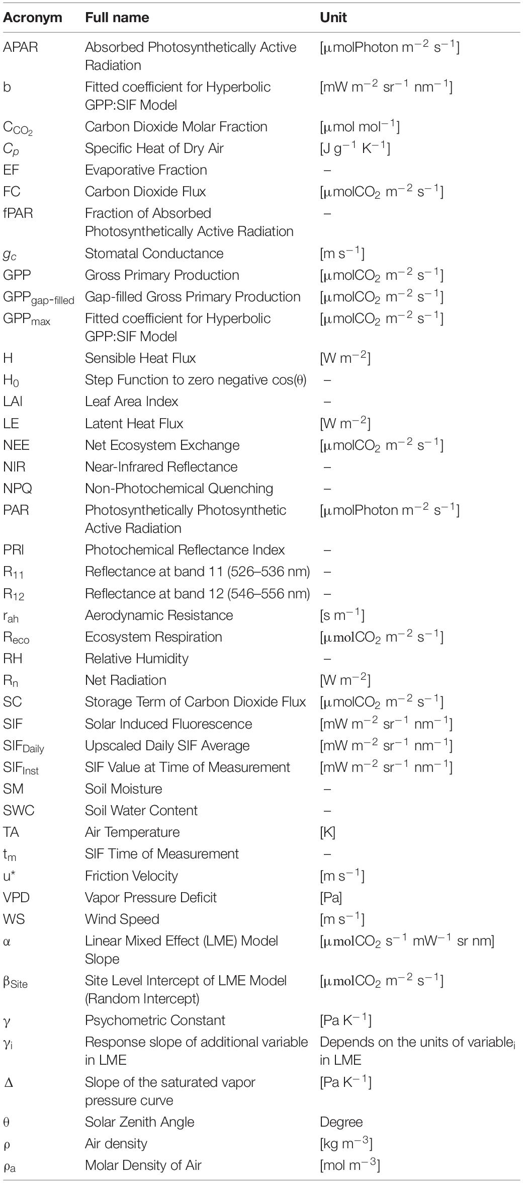
Table 1. Variable names, acronym definitions, and units.

Study Sites

Eddy covariance data were obtained through the AmeriFlux database¹, and the European Fluxes Database Cluster (EFDC)². This study was focused on temperate forest ecosystems located between 35°N and 65°N and considers the following IGBP land cover classifications: Evergreen Needleleaf Forests (ENF), Evergreen Broadleaf Forests (EBF), Deciduous Needleleaf Forests (DNF), Deciduous Broadleaf Forests (DBF), Mixed Forests (MF), and Woody Savannas (WSA). The study period comprised of growing seasons 2018 and 2019, depending on data availability from each site. We selected all sites that reported carbon dioxide fluxes for at least 50% of the year in 2018 and/or 2019. After filtering, 31 sites with 47 site-year growing seasons’ data were available for analysis: BE-Vie, CH-Lae, CZ-BK1, CZ-Lnz, CZ-RAJ, CZ-Stn, DE-Hai, DE-HoH, DE-Hzd, DE-Obe, DE-Tha, FR-Fon, IT-SR2, RU-Fyo, SE-Nor, US-Me2, US-Me6, US-MMS, US-NC3, US-NR1, US-PFa, US-Rpf, US-SRM, US-Syv, US-UMB, US-UMd, US-Vcm, US-WCr, YS-xBR, US-xDL, and US-xRM. Sites’ details (location on map, number of data points, DOI, coordinates, IGBP) were listed in Supplementary Material. Two sites provided hourly data instead of half-hourly (US-MMS and US-PFa), and in these sites data were interpolated to half-hourly for consistency.

Solar-Induced Chlorophyll Fluorescence Data

Solar-Induced Chlorophyll Fluorescence data were calculated from spectral observations by the TROPOspheric Monitoring Instrument (TROPOMI) satellite, launched on October 13th, 2017. TROPOMI spectral range met the 743–758 nm range for detecting SIF (Köhler et al., 2018), and was provided at a spatial resolution of 7 × 3.5 km² with global coverage. SIF emissions were detected daily at approximately same solar time (∼13:30 pm) at the equator. Swath time correction was applied at all sites in order to determine the local solar time for each observation. Overall SIF satellite measurements fell between 10 am and 2 pm local time. Observations obstructed by cloud-cover conditions were filtered out. SIF data were reported in milliwatt per meter squared, per steradian, per nanometer [mW m^–2 sr^–1nm^–1].

In order to get equivalent SIF values at the daily timescale, we used the scaling approach proposed by Frankenberg et al. (2011) to convert instantaneous SIF to daily average SIF. This method accounts for the variations in overpass time (including due to swath), length of day, and solar zenith angle:

$\begin{array}{c}SI{F}_{Daily}=SI{F}_{Inst}\times \frac{1}{\mathit{cos}(\mathrm{\theta }(t_m))}{\int }_{t=t_{m}12hours}^{t=t_m+12hours}\mathit{cos}(\mathrm{\theta }(t))\hfill \\ \times H_0\left(cos\left(\mathrm{\theta }\left(t\right)\right)\right)dt\hfill \end{array}(1)$

where SIF_Daily is the upscaled daily SIF average, SIF_Inst is the SIF value at time of measurement t_m, θ(t_m) is the corresponding solar zenith angle, and H₀ is a step function where H₀(cos(θ(t))) equals zero when cos(θ(t)) is negative and equals one when cos(θ(t)) is positive (Köhler et al., 2018). The integral is calculated using a time interval, dt, of 10 min.

Gross Primary Production Data

All sites reported turbulent net carbon dioxide fluxes (column FC, in the EC data), but Net Ecosystem Exchange (NEE) and GPP were not provided by all sites. For consistency, a unified modeling approach for estimating GPP was followed across all sites. NEE was calculated as the sum of the turbulent Flux of CO₂ (FC) and Storage of CO₂ (SC):

$\mathit{NEE}=\mathit{FC}+\mathit{SC}(2)$

Some of the sites did not provide SC, thus SC was approximated using the following equation:

$\mathit{SC}={\mathrm{\rho }}_a\times \underset{0}{\overset{h}{\int }}\frac{{\mathit{dC}}_{{\mathit{CO}}_2}}{\mathit{dt}}\mathit{dz}(3)$

where ρ_a is the molar density of the air [mol m^–3], and C_CO2 is Carbon Dioxide molar fraction [μmolmol^–1]. Integration includes all available measurements for carbon dioxide concentration from the ground to the CO₂ flux measurement height, h.

Growing Season

The growing season was defined using the carbon uptake period (i.e., carbon flux phenology, Garrity et al., 2011). A 7-day moving average of NEE was calculated and then, the peak seasonal NEE, i.e., the most negative 7-day average NEE for CO₂ uptake. The start and end of each site-year’s growing season were considered as the first and last day, respectively, where carbon uptake rates were above (more negative then) a threshold of 5% of the peak seasonal NEE. Growing season start and end dates of each site are provided in Supplementary Table 1.3. Following the identification of the time period of the growing season, a seasonal friction velocity (u*) filter threshold value was defined following the approach by Reichstein et al. (2005) and filtered flux data during times of low turbulence, below the u* threshold value.

Artificial Neural Network

An Artificial Neural Network (ANN) algorithm (Moffat et al., 2007), with parametric choices as described in Morin et al. (2014), was used to model fluxes during each growing season at each site. For each EC flux variable, 50% of valid observations were used to train the network, 25% of the remaining valid data to evaluate the network goodness of fit, and 25% to validate the final model. 100 networks were run per site-season, and the final model was the ensemble average of the top-fitting 10% of these. Separate ANN models were trained for daytime and nighttime data for each site-season.

During the process of modeling GPP, we first used an ANN to gap fill sensible heat (H) and latent heat (LE) fluxes. Then, an ANN was used to model ecosystem respiration (R_eco). It was assumed that during the night there was no photosynthetic activity, therefore, nighttime NEE was equal to R_eco. Thus, the ANN was trained with nighttime data. The resulting model was used to gap fill nighttime R_eco and NEE, and to simulate daytime R_eco. We assumed no nighttime GPP. The daytime was determined based on the Greenwich Mean Time (GMT) offset of each site and its latitude (Tramontana et al., 2020). During daytime, GPP was:

$\mathit{GPP}=\mathit{NEE}-R_{\mathit{eco}}(4)$

Where, during the daytime period of observations, GPP was a negative quantity and R_eco positive. This approach resulted in an observation gap whenever NEE observations were not available. We used these GPP data (corresponding with time when observed NEE values were available from EC and not gap-filled) for the half-hourly analysis. We used an ANN to gap fill NEE and used the complete time series of NEE and R_eco to calculate a gap-filled time series for GPP (GPP_gap–filled). Daily D and weekly GPP were calculated from GPP_gap–filled. The drivers of each of the ANN models for LE, H, R_eco, and GPP_gap–filled are listed in Table 2. It should be noted that PAR or net radiation, and soil moisture are usually used as GPP drivers, however, many sites did not report them and thus, requiring them as ANN input will lead to losing many sites for missing the corresponding data.

TABLE 2

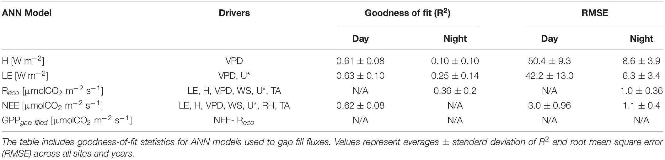
Table 2. Variables used as drivers in the ANN models used to gap fill different fluxes.

Ecosystem State Variables

Several environmental variables were used in the analysis along with SIF and GPP: canopy conductance (g_c), evaporative fraction (EF), APAR, photochemical reflectance index (PRI), PAR, soil moisture (SM), VPD, RH, TA, LE, fPAR, LAI, and NIR. All these variable data were provided using EC and remote sensing measurements or derived from data from EC measurements. Full descriptions for the source and calculation of each variable are listed below.

MODIS data product (MCD15A2H v006) was used for leaf area index (LAI) and fraction of absorbed PAR (fPAR), at 8-day time resolution and 500 m pixel size for each site using the Earthdata open-source repository³. APAR [μmolPhoton m^–2 s^–1] was calculated using the following equation:

$\mathit{APAR}=\mathit{fPAR}\times \mathit{PAR}(5)$

where PAR [μmolPhoton m^–2 s^–1] observations were measured at the EC flux sites.

Surface conductance was determined by inverting the Penman-Monteith model (Monteith, 1972) with measured evapotranspiration and meteorological data. The Penman-Monteith model separates the effects of aerodynamic and surface conductances. In forest ecosystems, where soil evaporation is small relative to leaf transpiration, the surface conductance is a good proxy for canopy conductance, g_c [m s^–1] (Novick et al., 2016), which, when the leaf surfaces do not hold standing water (as is the case most of the time, except immediately after precipitation), represents a volume-weighted integral of the leaf-level stomatal conductance. Noting that observation times around rain events are excluded from the analysis because no SIF measurements are available for thick cloud conditions, thus:

$g_c={\left[\frac{r_{\mathit{ah}}\times \mathrm{\Delta }\times R_n+\mathrm{\rho }\times C_p\times \mathit{VPD}}{\mathit{LE}\times \mathrm{\gamma }}-\frac{r_{\mathit{ah}}\times \left(\mathrm{\gamma }+\mathrm{\Delta }\right)}{\mathrm{\gamma }}\right]}^{-1}(6)$

where, r_ah is the water vapor aerodynamic resistance [s m^–1], Δ is the slope of the saturated vapor pressure curve [Pa K^–1], R_n is the net radiation [W m^–2], ρ is the air density [kg m^–3], C_p is specific heat of dry air [J g^–1 K^–1], VPD is the vapor pressure deficit [Pa], γ is the Psychometric constant [Pa K^–1], and LE is the latent heat flux [W m^–2] measured at the site. r_ah was approximated using site observations of u* and wind speed (ū) based on the empirical approach by Monteith and Unsworth (1990):

$r_{ah}=\frac{\overline{u}}{u^{{*}^2}}+\frac{6.2}{u^{{*}^{2/3}}}(7)$

Evaporative Fraction was also used as an indicator for water stress conditions, where it is the ratio of latent heat flux to the sum of latent heat flux and sensible heat flux, H [W m^–2]:

$EF=\frac{LE}{H+LE}(8)$

Surface soil water content (SWC) observations were provided by ground-based measurements (half hourly) at the EC sites, and from the spaceborne SMAP dataset⁴ at 6 am and 6 pm local time at daily basis. Both data sets were used separately in the analysis.

Photochemical Reflectance Index (PRI) is sensitive to changes in carotenoid pigments and used as an inverse proxy for NPQ at short timescales. MODIS data product (MYDOCGA, v006) is used to get reflectance at bands 11 and 12 at daily resolution and calculate a proxy of PRI at each site as described in Wang et al. (2020):

$PRI=\frac{R_{11}-R_{12}}{R_{11}+R_{12}}(9)$

where R₁₁ and R₁₂   are the reflectance at bands 11 (526–536 nm) and 12 (546–556 nm), respectively. MODIS data product (MOD13Q1 v006) was used for getting NIR. Table 1 above includes all the acronyms used in this study.

Data Analysis

Data analysis involves three timescales: half-hourly, daily, and weekly. Instantaneous SIF measurements are used for half-hourly timescale, upscaled daily average SIF values (Eq. 1) are used for the daily timescale, while weekly averages of SIF measurements are used for the weekly timescale. As for GPP, the half-hourly window during which a SIF observation was available is used for the half-hourly timescale, while daily and weekly averaged GPP_gap–filled values are used for the daily and weekly timescales, respectively. For all statistical inferences, a 0.05 significance level is considered.

The GPP:SIF relations was evaluated at multiple spatial scales and at the three temporal scales: half-hourly, daily, and weekly for each spatial scale. First, it was tested at the site level, where both a linear and a hyperbolic fit models were tested at each site.

Second, data were pooled across all sites and fitted using a linear regression model. Fourth, data were fitted using a Linear Mixed Effect (LME) model, where sites is considered as a random effect, SIF as a fixed effect, and GPP as the response variable:

$GPP\approx \mathrm{\alpha }\times SIF+{\mathrm{\beta }}_{Site}+{\mathrm{\gamma }}_{Site}\times SIF(10)$

where α is the SIF-driven slope (fixed slope), β_Site is the site-level intercept (random intercept), and γ_Site×SIF is the interaction between SIF and site. Third, we used similarly structured LME models, but added additional environmental variables as fixed effects using a forward stepwise regression for the LME model:

$GPP\approx \mathrm{\alpha }\times SIF+\sum _i\left({\mathrm{\gamma }}_i\times Variabl{e}_i\right)+{\mathrm{\beta }}_{Site}(11)$

where γ_i is the effect (response slope) of the ith environmental variable. Variables considered in the forward stepwise regression are: g_c, TA, SM, VPD, LAI, PRI, APAR, EF, LE, fPAR, and NIR. Variables were added to the model based on their pairwise R² with the residuals of the current model, and only if their addition decreased the Akaike Information Criterion (AIC; Hosmer et al., 2013).

To develop a more reliable estimate of GPP using solely remote sensing data sources, a simple decision tree model was developed where SIF was considered as a predictor of GPP along with other remote-sensing variables. These predictors included top-surface soil moisture estimates, LAI, PRI, fPAR, NIR, LE, and APAR calculated using MODIS products, which was calculated following Eq. 5, but with PAR retrieved from MODIS instead of PAR observations at the EC-tower location. Table 3 shows the source of each of the remote sensing product, in addition to their spatial resolution. For each variable, grids were aggregate consistent with a typical Eddy-Covariance footprint (1.5×1.5 km²). For variables with larger spatial resolution, spatial interpolation was used. Site and IGBP were included as categorical predictors in this selection-tree model in order to account for site characteristics. The contribution portion of each variable explaining GPP was used to indicate the relative importance of each variable in predicting GPP. The decision tree includes 50 layers, and 3 splits per tree. Twenty percent of the data was used for validation. It should be noted that this model was different from the LME or linear regression, as the decision tree did not assume the effects of the drivers to be linearly continuous. An important feature of decision tree models was allowing predictors’ classification by determining the contribution portion of each variable in predicting GPP.

TABLE 3

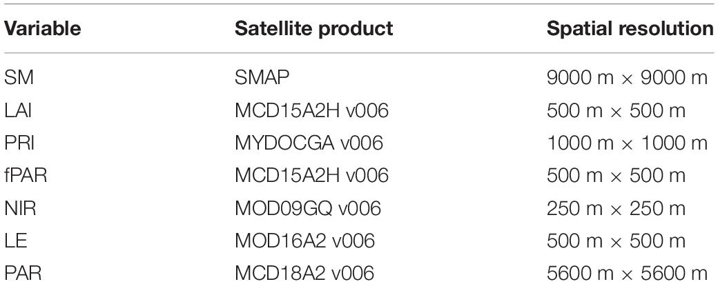
Table 3. Remote sensing products used in the decision tree model and their corresponding spatial resolution.

Throughout the processing of the results, MATLAB (2018) was used for data processing, ANN modeling, plotting, and pairwise and multiple linear regressions. JMP Pro 14 was used for statistical inference using a general mixed-effect linear models (LME), and for the decision-tree model (JMP, 2018; MATLAB, 2018).

Results

Gross Primary Production vs. Solar-Induced Chlorophyll Fluorescence at Each Site

At the half-hourly timescale, only 19% of the sites showed significant pairwise linear correlations between GPP and SIF. At the daily timescale, 52% of the sites showed significant correlation between GPP and SIF, and at the weekly timescale, 42% of the sites showed a significant correlation (Supplementary Table 1.2). The highest goodness of fit at all timescales was reached at the site SE-Nor, where weekly data had the highest R² of 0.66 (Figure 1). The number of data points for each fit ranged between 10 and 60, depending on the data availability at each site. The detailed results and statistics for each site are shown in Supplementary Material.

FIGURE 1

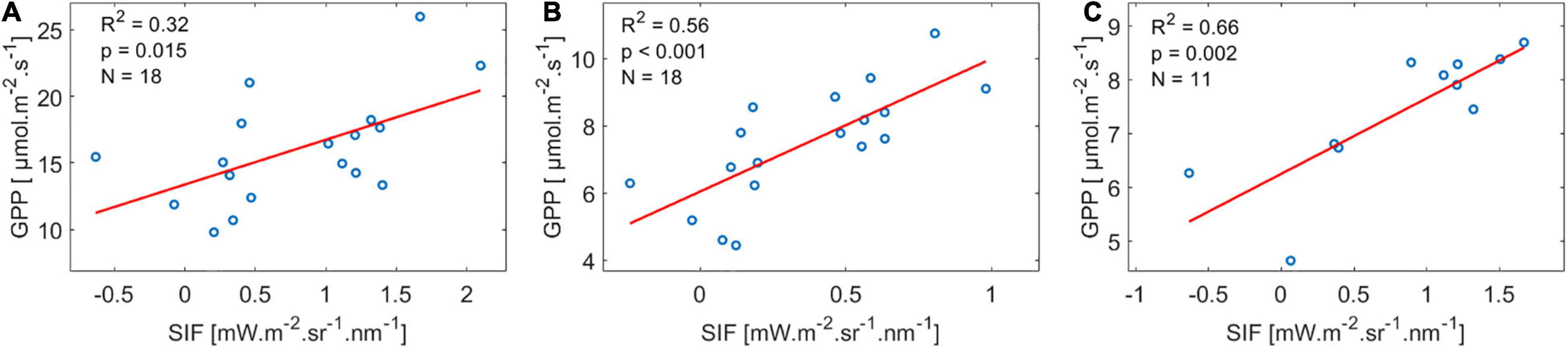
Figure 1. Example for GPP:SIF relations, using data from SE-Nor, where GPP:SIF had the best goodness of fit at the site level. (A) Half-Hourly, (B) Daily, and (C) Weekly timescales. The red line represents the linear regression fit.

Alternatively, we tested the regression between GPP and SIF at half-hourly resolution assuming a hyperbolic relationship, following Damm et al. (2015):

$GPP=GP{P}_{max}\times \frac{SIF}{SIF+b}(12)$

where GPP_max and b were fitting coefficients. This resulted in only two sites showing a significant but very weak relationship (Figure 2).

FIGURE 2

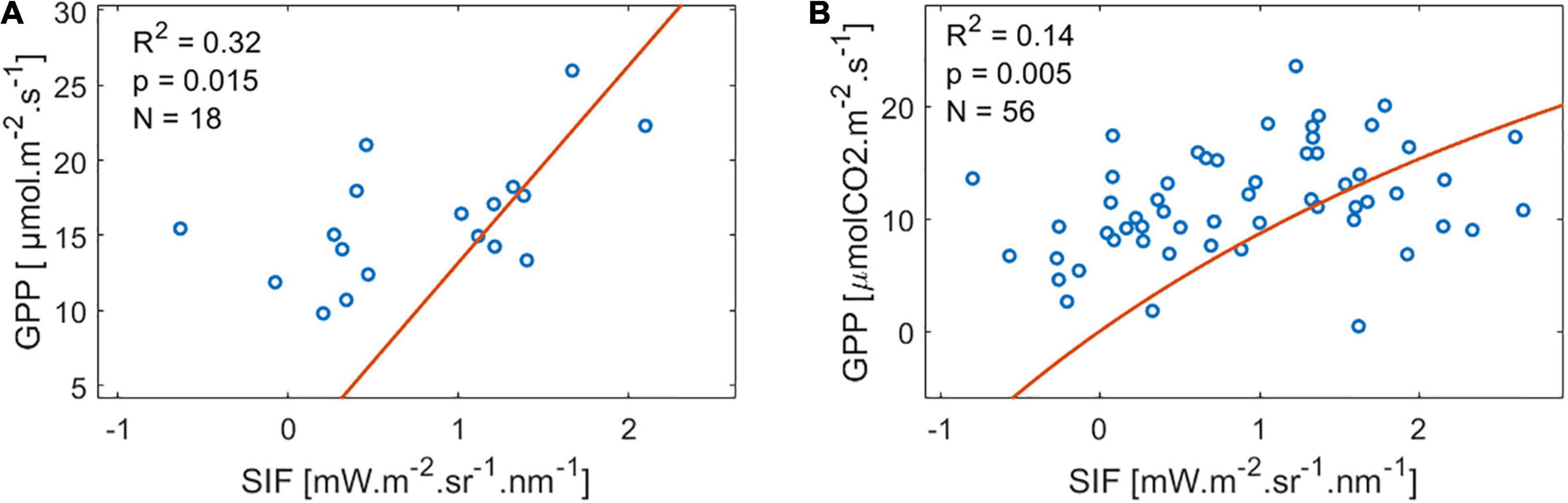
Figure 2. Results of the sites with a significant hyperbolic correlation at half-hourly resolution. Significant correlation happened at (A) SE-Nor and (B) US-Me2. The red line represents the hyperbolic fit.

Gross Primary Production vs. Solar-Induced Chlorophyll Fluorescence Over All Sites

We tested the linear relationship between GPP and SIF, pooled across all sites of the same IGBP classification. No significant relationship was found for all sites, while a very weak correlation was found for ENF and DBF (Figure 3). As for MF a weak (R² = 0.09) but significant negative linear regression between GPP and SIF was found. However, this was due to the fact that data were clustered by site within the MF biome (Figure 3D), where some sites, such as CZ-Lnz and BE-Vie, had high GPP but low SIF relative to other sites, leading to an overall apparent negative GPP:SIF relations in this biome. Similar results were found for daily and weekly timescales.

FIGURE 3

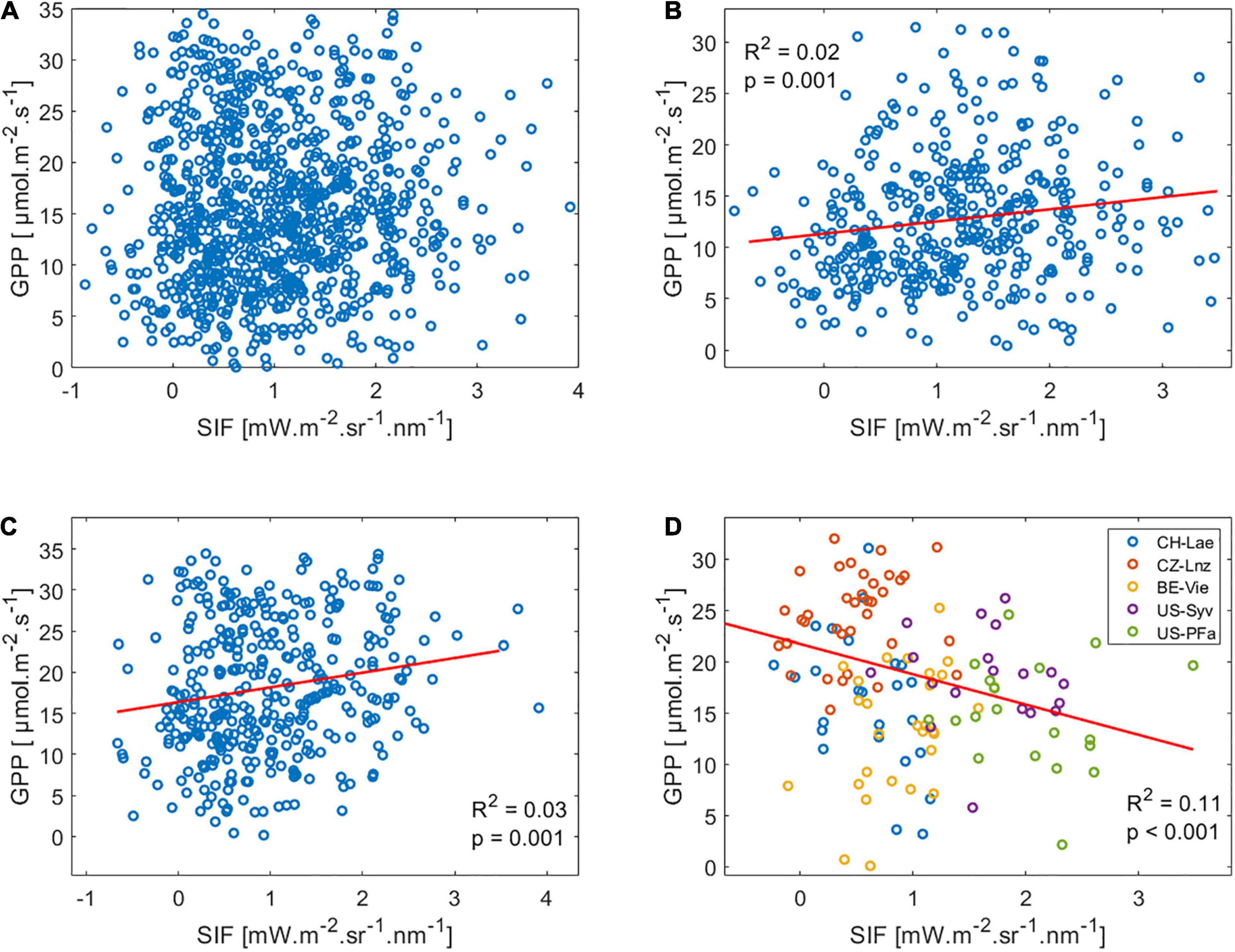
Figure 3. GPP:SIF correlation for half-hourly data for (A) all 31 sites plotted together, (B) ENF sites, (C) DBF sites, and (D) MF sites. Red line represents the linear regression fit. A regression line is not shown where the regression is not significant.

When we included the variation between sites as a random effect (Site) in a LME, the resulting GPP:SIF correlation was highly significant, whereas the interaction term between SIF and site (i.e., assuming there was a different GPP:SIF slope at each site in addition to different intercepts) was found not to have a significant effect, and therefore was not included in the final model (Figure 4).

FIGURE 4

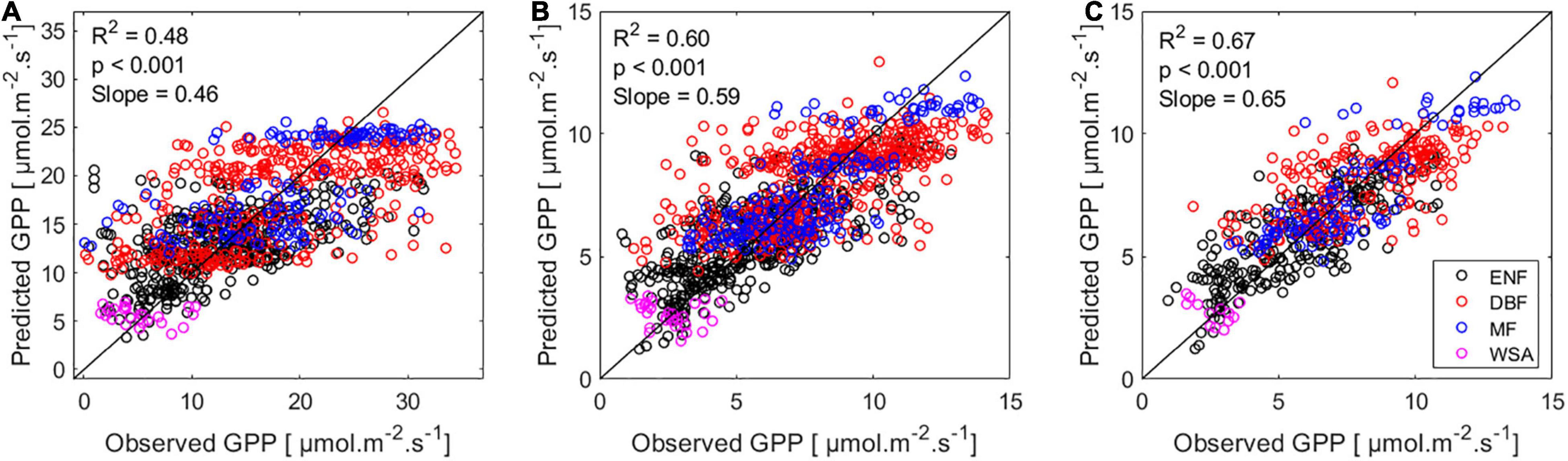
Figure 4. Linear mixed effect model fit based on SIF data for (A) Half-Hourly, (B) Daily, and (C) Weekly timescales. The x-axis show the observed GPP, i.e., half-hourly EC GPP for (A), mean daily GPP for (B), and mean weekly GPP for (C). The y-axis show GPP values predicted by the LME model. The black line represents the 1:1 line.

The effect of adding other environmental variables, in addition to SIF, as predictors for GPP was significant, but with different results among timescales (Table 3). It was found that water-status related variables, g_c, LE, and EF had the strongest impact on the goodness of fit (evaluated in terms of improvement in correlation R²) of the GPP at all three timescales. Daily and weekly timescales were characterized by having a set of environmental variables that improved the relationship between GPP and SIF, namely variables related to phenology and canopy structure (g_c, LAI, fPAR, NIR, and APAR), which was not the case for the half-hourly model.

It should be noted that many of the different environmental variables involved in the analysis are inter-correlated, particularly those related to leaf color that vary with a similar seasonal phenological pattern, i.e., LAI, fPAR, and NIR. Nevertheless, each of these might have an independent component in its information content regarding GPP:SIF. In the forward stepwise regression, we sorted the variables in order of their pairwise regression with the residuals of GPP:SIF. We then added each element in order to the multivariate regression model. A variable that was perfectly correlated to another variable already included in the model would not have any information content remaining to improve the model. Our model showed that LAI, fPAR, and NIR all added a significant information components to the model at both daily and weekly timescales. These three variables were therefore, further considered in the more complex decision tree model.

In order to further test the influence of g_c and canopy on the empirical relationship between GPP and SIF, the distribution of the LME model errors of GPP vs. SIF (expressed as model residuals = observations – model predictions) is studied under low (the lowest 33% at each site), intermediate (33th to 67th percentile per site), and high (highest 33% at each site) g_c and fPAR separately (Figure 5).

FIGURE 5

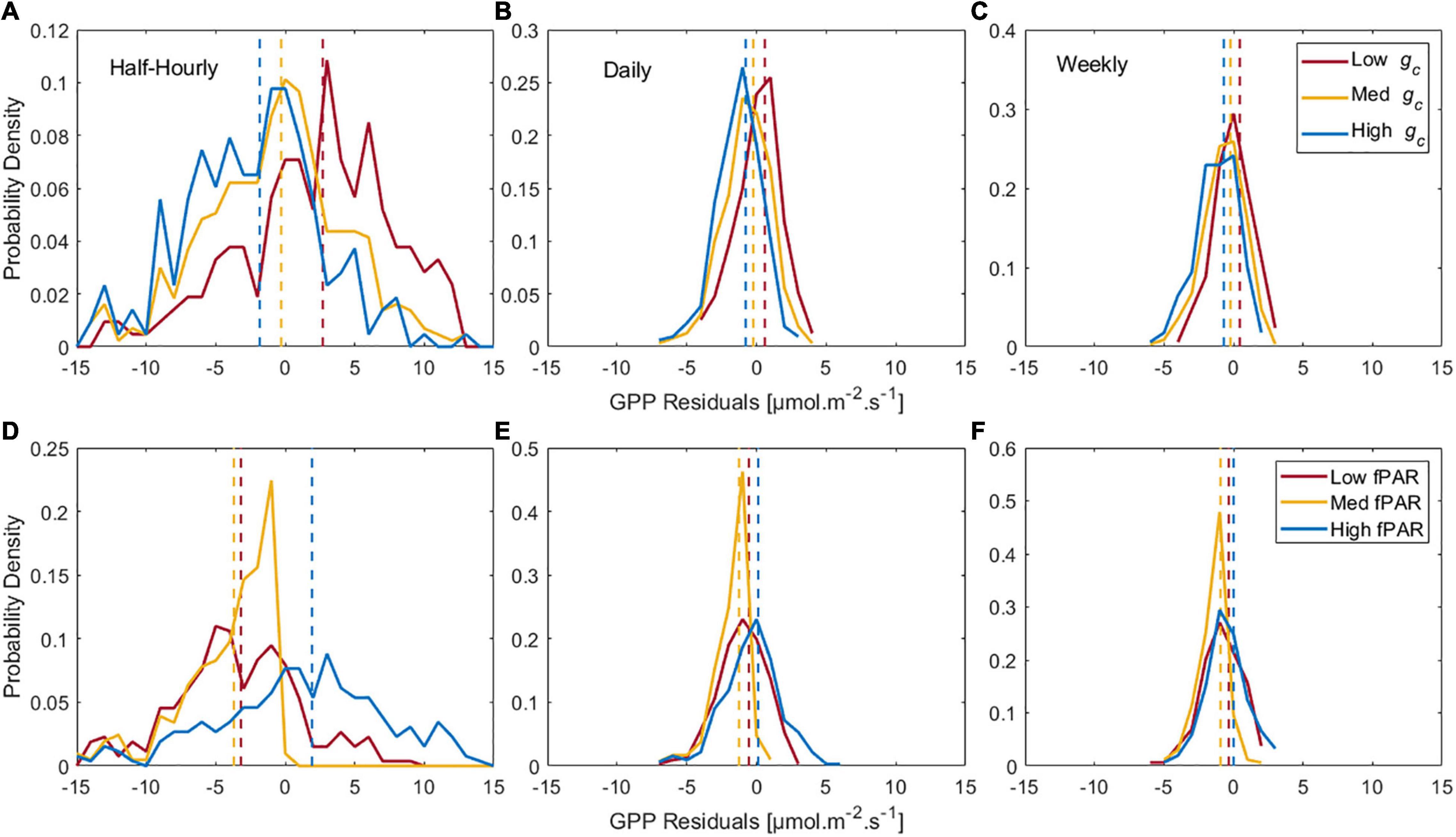
Figure 5. Probability density function of the LME model residuals (observation-model) for GPP as a function of SIF (fixed effect) and site (random effect) under low, intermediate, and high canopy conductance (0–33th percentile, 33th–67th, and 67th–100th percentiles of g_c values within each site, respectively) at (A) Half-hourly, (B) Daily, and (C) Weekly timescales. Distribution density function of the residuals (observation-model) of the same model under low, intermediate, and high fPAR (0–33th percentile, 33th–67th, and 67th–100th percentiles of fPAR values within each site, respectively) at (D) Half-hourly, (E) Daily, and (F) Weekly timescales. Dashed lines at the same color represent the mean of each distribution.

The decision-tree model shows that sites has the highest contribution to predicting GPP among other remote sensing predictors, while SIF has a minimal contribution, along with IGBP, PRI, SM, and fPAR. APAR, LAI, LE, and NIR showed a relatively high contribution with divergence in contribution portions across timescale (Figure 6). Model precision (estimated through R²) increased with decreasing temporal resolution.

FIGURE 6

Figure 6. Decision-tree model results showing the contribution portion of each variable in predicting GPP at the three timescales and the corresponding sample size (n), root mean square error (RMSE), and R² of the training and validation data sets.

Discussion

Other studies of GPP:SIF using EC method and remote sensing (e.g., Li et al., 2018b) showed stronger and more consistent GPP:SIF correlations than the ones we found. We hypothesize that the main reason for this difference in the goodness of fit of the SIF models is that our study focused on the inter-daily and inter-weekly variation within the growing season. Therefore, diurnal and seasonal variations of GPP and SIF, which are stronger and more predictable than the inter-daily variations, are not emphasized in this study. Our findings that weekly and daily average GPP are better correlated to SIF than half-hourly GPP are consistent with earlier studies, which have shown a stronger linear relationship at lower temporal resolution. This trend across timescales indicates that SIF is a good predictor for seasonal variations of GPP (Magney et al., 2019), but not necessarily for the instantaneous photochemical activity (Magney et al., 2020). Site-level analysis shows limited relationship between SIF and GPP at midday, half-hourly resolution using both linear and asymptotic fits, while it is expected to have a hyperbolic correlation at this time of day. This can be due to light saturation that dominates midday photosynthesis under most conditions (Zhang et al., 2016a). Thus, TROPOMI-sampled points at solar noon would lie mostly on the asymptotic end of the GPP vs. SIF hypothetical non-linear curve (Damm et al., 2015). In order to get the hypothetical non-linear correlation between GPP and SIF, data points with minimal light saturation are needed to complement the hyperbolic shape of the curve, i.e., morning SIF data should be available, which is not the case with TROPOMI, or midday data with less stress conditions.

It is possible that variability in species specific parameters that governs GPP:SIF creates high levels of within-site variation in species-rich and heterogeneous sites. If this hypothesis is true, the sites with the strong GPP:SIF correlation are expected to be the ones that have the lowest species diversity. Indeed, such is the case in some sites, for example SE-Nor is composed of only pine and spruce (Lindroth et al., 1998), CZ-BK1 and CZ-RAJ are composed of monoculture Norway spruce (Sedlák et al., 2010; McGloin et al., 2018), in BE-Vie three species represent more than 80% of vegetation (Aubinet et al., 2001), and US-NC3 is composed almost exclusively of loblolly pine (Yang Y. et al., 2017). However, other sites, where GPP and SIF are significantly and strongly correlated, are among the most diverse. For example, US-UMB has seven different species with relatively equal dominance among three of them (Matheny et al., 2014), RU-Fyo has 49% of spruce, 12% of pine forests, 28% birch, 14% aspen, and 1% alder (Sogachev et al., 2002). The site descriptions in AmeriFlux and EFDC do not enable calculating a formal species diversity index for each site, and we could not test the significance of the assumed negative relationship between species diversity and GPP:SIF goodness of fit. Nonetheless, we investigated the community-composition complexity using the spatial heterogeneity of LAI (similar to the approach by Chu et al., 2021). This quantity is an indirect estimation of the variation in vegetation structure, and could be used as an indirect proxy for the diversity of the dominant species. The coefficient of variability for LAI (using spatial standard deviation) was provided by the MODIS MCD15A2H product at each site. LAI values were calculated at a 1.5 × 1.5 km² spatial resolution, which is close to a typical EC footprint. We found no significant relationship between the R² of site-level GPP:SIF correlations and the LAI coefficient of variability (plots and detailed results are shown in Supplementary Material). It should be noted that the LAI coefficient of variability is an indicator of overstory dominant species, thus neglecting the effect of understory species, which would significantly contribute to the total fluorescence signal when light conditions allow.

Another hypothetical cause of the low correlation between GPP and SIF may be the lack of representativeness of the SIF pixel relative to the EC-flux footprint (Chu et al., 2021). While these land cover overlap, but potentially different areas, it is possible that species specific response within the EC-footprint captures a somewhat different evapotranspiration dynamic than the SIF pixel. However, the finding that the spatial variability of LAI is not correlated with the goodness of fit of GPP:SIF is indicative that low footprint representativeness (typical to sites with high LAI variation) is not the lead cause of the low GPP:SIF fit. Furthermore, TROPOMI offers a higher resolution (7 × 3.5 km²) compared than other satellites that provide SIF data, such as GOME that has a resolution of 80 × 40 km², and a better spatial coverage than OCO-2 which have a higher spatial resolution of 2 × 1.3 km² (Köhler et al., 2018).

Given the lack of significant effect of within-site vegetation heterogeneity, we hypothesize that site-specific environmental and structural conditions (water status, canopy structure, degree of isohydricity, soil texture) are probably more important in driving GPP:SIF than the ecosystem characteristics that classify its IGBP type or its species richness and heterogeneity (Zhang et al., 2018c; Dechant et al., 2020). This hypothesis is further supported by the LME models results, which show a strong variability in GPP:SIF relations among sites, and the decision tree model, which shows that Site is the main contributor to GPP prediction. Li et al. (2020) shows that the linear GPP:SIF relations is affected by the growth stages of maize during the growing season. Migliavacca et al. (2017) shows that the relationship is a function of nutrient addition (Nitrogen, and Phosphorous), which induces changes in canopy structure and functional traits. We find that the size of the site-specific random effect in the LME model can be predicted by the site-level mean LAI, fPAR and canopy conductance at all timescales (Figure 7). A multiple-linear regression of sites’ intercept with LAI and g_c together yielded an R² of 0.56 and the interaction between g_c and LAI was not significant. This result further substantiates the hypothesis that both canopy structure and plant function control GPP:SIF, to a large degree, and offers hope for effectively predicting the site-level intercept that is needed for the global applicability of GPP:SIF (Dechant et al., 2020; Kim et al., 2021).

FIGURE 7

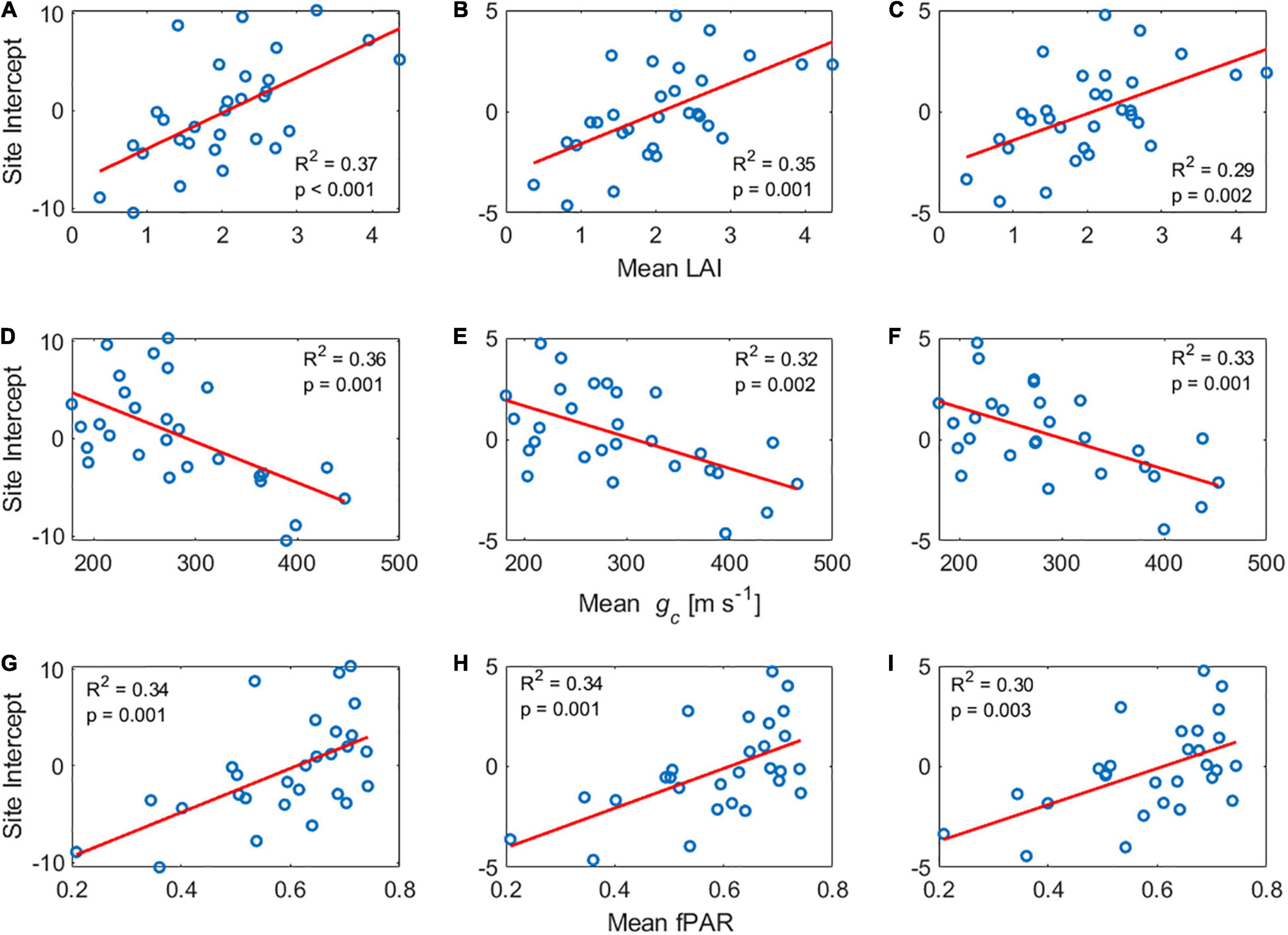
Figure 7. Site-level intercept estimated by LME vs. Mean LAI for (A) Hourly, (B) Daily, and (C) Weekly timescales. Site-level intercept estimated by LME vs. Mean g_c for (D) Hourly, (E) Daily, and (F) Weekly timescales. Site-level intercept estimated by LME vs. Mean fPAR for (G) Hourly, (H) Daily, and (I) Weekly timescales. The red line represents the linear regression fit.

Table 4 shows that water stress indicators, provide significant improvement to the GPP:SIF correlation among other environmental variables at all timescales. Water stress variables, specifically stomatal conductance significantly improved the model at all timescales. Phenology indicators (LAI, NIR, and fPAR) and APAR improve GPP:SIF at daily and weekly resolutions, which is in agreement with earlier studies, notably Magney et al. (2020), but not at half hourly resolution. Contrary to our expectations and earlier findings (Helm et al., 2020; Marrs et al., 2020), we found that the GPP:SIF LME model is over-estimating GPP under high and intermediate g_c (Figures 5A–C) and underestimating GPP under low g_c. Overestimation of GPP happens at low and intermediate fPAR at the half-hourly timescale. SIF is driven by canopy properties like chlorophyll content, LAI, and angle distribution of leaves more than by canopy biochemistry (Frankenberg and Berry, 2018). At high chlorophyll content, light absorption per unit of chlorophyll decreases, thus resulting in a non-linear relationship between chlorophyll content and light absorption (Porcar-Castell et al., 2014). In such case, a high SIF signal is expected to overestimate GPP. Since our study focuses on the growing season, high chlorophyll content governs the state of vegetation, resulting in GPP overestimation under low and intermediate fPAR. This effect can also be responsible for the overestimation of GPP under high stomata conductance. At low fPAR, low GPP is driven by low APAR instead of stomatal conductance.

TABLE 4

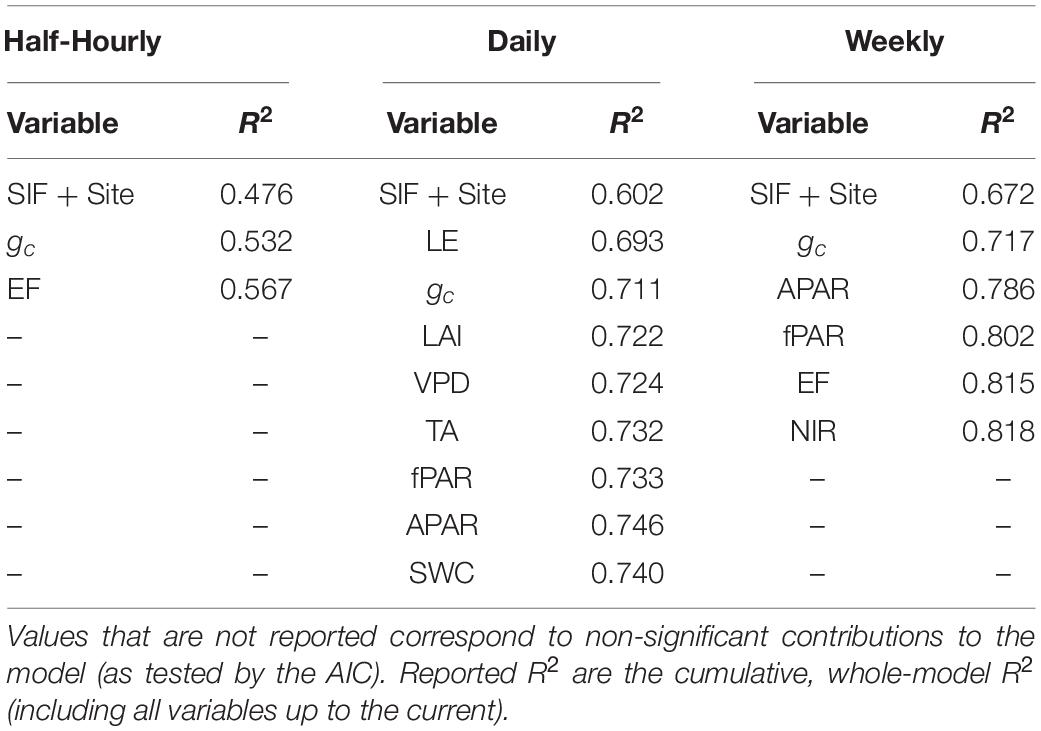
Table 4. Effects of environmental variables on the goodness-of-fit of LME of GPP vs. SIF using forward stepwise regression.

The decision-tree model considered only remote sensing variables as GPP predictors in addition to site. The model results identified the strong effect of inter-site variability in predicting GPP. It also found low contribution of SIF to GPP predictability, compared to other variables. However, surprisingly, the decision-tree model resulted in an overall similar performance as the GPP:SIF LME model when comparing the R² of the two models at each timescale (Table 5 and Figure 4). We hypothesize that the strong cross-correlation of many environmental variables have limited the information content of the overall ensemble of variables and explains the similar goodness of fit of these two very different models. Decision-tree model results emphasized the role of variables indicative of canopy structure (NIR, APAR, and LAI) and water status (LE) in supplementing SIF-based prediction of GPP, noting that fPAR showed a lower contribution portion probably due to its high covariance with LAI.

TABLE 5

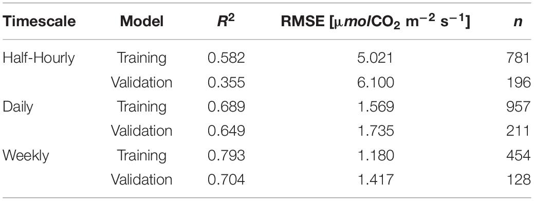
Table 5. Decision tree model statistics.

Conclusion

Our study evaluates spaceborne SIF from TROPOMI as a predicting variable for inter-daily variation of GPP during the growing season in 31 EC sites. A strong inter-site variability in the intercept of GPP:SIF regression is found. The need for site-specific intercepts as coefficients in a model for accurately predicting GPP from SIF limits the applicability of SIF as a globally observable surrogate of GPP. However, our results suggest that this intercept is driven by canopy structure and site-level vegetation function and is predictable using site-level, season-long, mean fPAR, LAI, and canopy conductance. These latter showed as well to significantly improve the LME model at all timescales. Thus, canopy structure and water status variables at site level are important factors to account for when using SIF as a predictor of GPP intra-daily variations.

Data Availability Statement

Observations of carbon fluxes and other site-level meteorological variables are available through Amerilfux (https://ameriflux.lbl.gov/data/aboutdata/) and European Fluxes Database Cluster (EFDC) (http://www.europe-fluxdata.eu/home/data/data-policy). All Site IDs and DOIs for all sites used are listed in Table S1.1 in Supplementary Material 1. MODIS datasets MCD15A2H v006, MCD18A2 v006, MOD13Q1 v006, MOD16A2 v006, and MYDOCGA v006 provide LAI and fPAR, PAR, PRI, NIR, LE, and PRI data and are available through NASA’s EarthData (https://search.earthdata.nasa.gov/search). SMAP soil moisture data are available through the National Snow and Ice Data Center (NSIDC) (https://nsidc.org/data/smap). SIF data from the TROPOMI satellite are available through (http://www.tropomi.eu/data-products/data-access). Merged datasets, with the modeled, site-level, GPP and SIF values, and other environmental variables that were used in the analysis at half-hourly, daily, and weekly timescales are provided in Supplementary Material 3–5.

Author Contributions

TY performed the data analyses and prepared the figures. TY and GB led the writing of the manuscript. GB and PG conceived the idea of the manuscript. LY processed TROPOMI data. NA, CB, PB, AD, DD, AK, NK, SM, MM, AN, KN, RS, LŠ, KS, MU, and AV contributed to EC data. All authors discussed the results and participated in writing and editing of the manuscript.

Funding

Funding for this study and for Ameriflux core sites was provided by the United States Department of Energy’s Office of Science through the Ameriflux Management Project. MU was partially supported by the Arctic Challenge for Sustainability II (ArCS II; JPMXD1420318865). LŠ was supported by the Ministry of Education, Youth and Sports of CR within Mobility CzechGlobe2 (CZ.02.2.69/0.0/0.0/18_053/0016924). Site-level data are provided by AmeriFlux and the European Fluxes Database Cluster. The National Ecological Observatory Network (NEON) is sponsored by the National Science Foundation and operated under cooperative agreement by Battelle Memorial Institute.

Conflict of Interest

The authors declare that the research was conducted in the absence of any commercial or financial relationships that could be construed as a potential conflict of interest.

Publisher’s Note

All claims expressed in this article are solely those of the authors and do not necessarily represent those of their affiliated organizations, or those of the publisher, the editors and the reviewers. Any product that may be evaluated in this article, or claim that may be made by its manufacturer, is not guaranteed or endorsed by the publisher.

Acknowledgments

We thank Philipp Koehler and Christian Frankenberg at Caltech for providing TROPOMI SIF data and Olya Skulovish for processing SMAP data. We also thank the two reviewers who assisted in reviewing the manuscript.

Supplementary Material

The Supplementary Material for this article can be found online at: https://www.frontiersin.org/articles/10.3389/ffgc.2021.695269/full#supplementary-material

Footnotes

1. ^ https://ameriflux.lbl.gov/
2. ^ http://www.europe-fluxdata.eu/
3. ^ https://search.earthdata.nasa.gov/
4. ^ https://nsidc.org/data/smap

References

Aubinet, M., Chermanne, B., Vandenhaute, M., Longdoz, B., Yernaux, M., and Laitat, E. (2001). Long Term Carbon Dioxide Exchange above a Mixed Forest in the Belgian Ardennes. Agric. For. Meteorol. 108, 293–315. doi: 10.1016/S0168-1923(01)00244-1

CrossRef Full Text | Google Scholar

Baker, N. R. (2008). Chlorophyll Fluorescence: a Probe of Photosynthesis in Vivo. Annu. Rev. Plant Biol. 59, 89–113. doi: 10.1146/annurev.arplant.59.032607.092759

PubMed Abstract | CrossRef Full Text | Google Scholar

Balzarolo, M., Valdameri, N., Fu, Y. H., Schepers, L., Janssens, I. A., and Campioli, M. (2019). Different Determinants of Radiation Use Efficiency in Cold and Temperate Forests. Glob. Ecol. Biogeogr. 28, 1649–1667. doi: 10.1111/geb.12985

CrossRef Full Text | Google Scholar

Chang, C. Y., Guanter, L., Frankenberg, C., Köhler, P., Gu, L., Magney, T. S., et al. (2020). Systematic Assessment of Retrieval Methods for Canopy Far-Red Solar-Induced Chlorophyll Fluorescence Using High-Frequency Automated Field Spectroscopy. J. Geophys. Res. Biogeosci. 125, 1–26. doi: 10.1029/2019JG005533

CrossRef Full Text | Google Scholar

Chen, J., Liu, X., Du, S., Ma, Y., and Liu, L. (2020). Integrating Sif and Clearness Index to Improve Maize GPP Estimation Using Continuous Tower-Based Observations. Sensors 20:2493. doi: 10.3390/s20092493

PubMed Abstract | CrossRef Full Text | Google Scholar

Chu, H., Luo, X., Ouyang, Z., Chan, W. S., Dengel, S., Biraud, S. C., et al. (2021). Representativeness of Eddy-Covariance Flux Footprints for Areas Surrounding AmeriFlux Sites. Agric. For. Meteorol. 301–302, 108350. doi: 10.1016/j.agrformet.2021.108350

CrossRef Full Text | Google Scholar

Damm, A., Guanter, L., Paul-Limoges, E., van der Tol, C., Hueni, A., Buchmann, N., et al. (2015). Far-Red Sun-Induced Chlorophyll Fluorescence Shows Ecosystem-Specific Relationships to Gross Primary Production: an Assessment Based on Observational and Modeling Approaches. Remote Sens. Environ. 166, 91–105. doi: 10.1016/j.rse.2015.06.004

CrossRef Full Text | Google Scholar

Dechant, B., Ryu, Y., Badgley, G., Zeng, Y., Berry, J. A., Zhang, Y., et al. (2020). Canopy Structure Explains the Relationship between Photosynthesis and Sun-Induced Chlorophyll Fluorescence in Crops. Remote Sens. Environ. 241:111733. doi: 10.1016/j.rse.2020.111733

CrossRef Full Text | Google Scholar

Du, S., Liu, L., Liu, X., Guo, J., Hu, J., Wang, S., et al. (2019). SIFSpec: measuring Solar-Induced Chlorophyll Fluorescence Observations for Remote Sensing of Photosynthesis. Sensors 19:3009. doi: 10.3390/s19133009

PubMed Abstract | CrossRef Full Text | Google Scholar

Flexas, J., Díaz-Espejo, A., Conesa, M. A., Coopman, R. E., Douthe, C., Gago, J., et al. (2016). Mesophyll Conductance to CO2 and Rubisco as Targets for Improving Intrinsic Water Use Efficiency in C3 Plants. Plant Cell Environ. 39, 965–982. doi: 10.1111/pce.12622

PubMed Abstract | CrossRef Full Text | Google Scholar

Frankenberg, C., and Berry, J. (2018). Solar Induced Chlorophyll Fluorescence: origins, Relation to Photosynthesis and Retrieval. Compr. Remote Sens. 3, 143–162. doi: 10.1016/B978-0-12-409548-9.10632-3

CrossRef Full Text | Google Scholar

Frankenberg, C., Fisher, J. B., Worden, J., Badgley, G., Saatchi, S. S., Lee, J. E., et al. (2011). New Global Observations of the Terrestrial Carbon Cycle from GOSAT: patterns of Plant Fluorescence with Gross Primary Productivity. Geophys. Res. Lett. 38, 1–6. doi: 10.1029/2011GL048738

CrossRef Full Text | Google Scholar

Garrity, S. R., Bohrer, G., Maurer, K. D., Mueller, K. L., Vogel, C. S., and Curtis, P. S. (2011). A Comparison of Multiple Phenology Data Sources for Estimating Seasonal Transitions in Deciduous Forest Carbon Exchange. Agric. For. Meteorol. 151, 1741–1752. doi: 10.1016/j.agrformet.2011.07.008

CrossRef Full Text | Google Scholar

Goulas, Y., Fournier, A., Daumard, F., Champagne, S., Ounis, A., Marloie, O., et al. (2017). Gross Primary Production of a Wheat Canopy Relates Stronger to Far Red Than to Red Solar-Induced Chlorophyll Fluorescence. Remote Sens. 9:97. doi: 10.3390/rs9010097

CrossRef Full Text | Google Scholar

Grassi, G., and Magnani, F. (2005). Stomatal, Mesophyll Conductance and Biochemical Limitations to Photosynthesis as Affected by Drought and Leaf Ontogeny in Ash and Oak Trees. Plant Cell Environ. 28, 834–849. doi: 10.1111/j.1365-3040.2005.01333.x

CrossRef Full Text | Google Scholar

Green, J. K., Berry, J., Ciais, P., Zhang, Y., and Gentine, P. (2020). Amazon Rainforest Photosynthesis Increases in Response to Atmospheric Dryness. Sci. Adv. 6:eabb7232. doi: 10.1126/sciadv.abb7232

PubMed Abstract | CrossRef Full Text | Google Scholar

Grossiord, C., Buckley, T. N., Cernusak, L. A., Novick, K. A., Poulter, B., Siegwolf, R. T. W., et al. (2020). Plant Responses to Rising Vapor Pressure Deficit. New Phytol. 226, 1550–1566. doi: 10.1111/nph.16485

PubMed Abstract | CrossRef Full Text | Google Scholar

Gu, L., Han, J., Wood, J. D., Chang, C. Y. Y., and Sun, Y. (2019). Sun-Induced Chl Fluorescence and Its Importance for Biophysical Modeling of Photosynthesis Based on Light Reactions. New Phytol. 223, 1179–1191. doi: 10.1111/nph.15796

PubMed Abstract | CrossRef Full Text | Google Scholar

Guan, K., Berry, J. A., Zhang, Y., Joiner, J., Guanter, L., Badgley, G., et al. (2016). Improving the Monitoring of Crop Productivity Using Spaceborne Solar-Induced Fluorescence. Glob. Chang. Biol. 22, 716–726. doi: 10.1111/gcb.13136

PubMed Abstract | CrossRef Full Text | Google Scholar

Guan, K., Wu, J., Kimball, J. S., Anderson, M. C., Frolking, S., Li, B., et al. (2017). The Shared and Unique Values of Optical, Fluorescence, Thermal and Microwave Satellite Data for Estimating Large-Scale Crop Yields. Remote Sens. Environ. 199, 333–349. doi: 10.1016/j.rse.2017.06.043

CrossRef Full Text | Google Scholar

Guanter, L., Zhang, Y., Jung, M., Joiner, J., Voigt, M., Berry, J. A., et al. (2014). Global and Time-Resolved Monitoring of Crop Photosynthesis with Chlorophyll Fluorescence. Proc. Natl. Acad. Sci. U. S. A. 111, E1327–E1333. doi: 10.1073/pnas.1320008111

PubMed Abstract | CrossRef Full Text | Google Scholar

He, L., Wood, J. D., Sun, Y., Magney, T., Dutta, D., Köhler, P., et al. (2020b). Tracking Seasonal and Interannual Variability in Photosynthetic Downregulation in Response to Water Stress at a Temperate Deciduous Forest. J. Geophys. Res. Biogeosci. 125, 1–23. doi: 10.1029/2018jg005002

CrossRef Full Text | Google Scholar

He, L., Magney, T., Dutta, D., Yin, Y., Köhler, P., Grossmann, K., et al. (2020a). From the Ground to Space: using Solar-Induced Chlorophyll Fluorescence to Estimate Crop Productivity. Geophys. Res. Lett. 47, 1–12. doi: 10.1029/2020GL087474

CrossRef Full Text | Google Scholar

Helm, L. T., Shi, H., Lerdau, M. T., and Yang, X. (2020). Solar-Induced Chlorophyll Fluorescence and Short-Term Photosynthetic Response to Drought. Ecol. Appl. 30:e02101. doi: 10.1002/eap.2101

PubMed Abstract | CrossRef Full Text | Google Scholar

Hosmer, D. W., Lemeshow, S., and Sturdivant, R. X. (2013). “Model-Building Strategies and Methods for Logistic Regression,” in Applied logistic regression, Third Ed, 3rd Edn, eds D. W. Hosmer Jr., S. Lemeshow and R. X. Sturdivant (Hoboken, NJ, USA: John Wiley & Sons, Inc), 89–151. doi: 10.1002/9781118548387.ch4

CrossRef Full Text | Google Scholar

Jeong, S. J., Schimel, D., Frankenberg, C., Drewry, D. T., Fisher, J. B., Verma, M., et al. (2017). Application of Satellite Solar-Induced Chlorophyll Fluorescence to Understanding Large-Scale Variations in Vegetation Phenology and Function over Northern High Latitude Forests. Remote Sens. Environ. 190, 178–187. doi: 10.1016/j.rse.2016.11.021

CrossRef Full Text | Google Scholar

JMP (2018). JMP Pro. Cary, NC: SAS Institute Inc.

Google Scholar

Joiner, J., Yoshida, Y., Vasilkov, A. P., Schaefer, K., Jung, M., Guanter, L., et al. (2014). The Seasonal Cycle of Satellite Chlorophyll Fluorescence Observations and Its Relationship to Vegetation Phenology and Ecosystem Atmosphere Carbon Exchange. Remote Sens. Environ. 152, 375–391. doi: 10.1016/j.rse.2014.06.022

CrossRef Full Text | Google Scholar

Jonard, F., De Cannière, S., Brüggemann, N., Gentine, P., Short Gianotti, D. J., Lobet, G., et al. (2020). Value of Sun-Induced Chlorophyll Fluorescence for Quantifying Hydrological States and Fluxes: current Status and Challenges. Agric. For. Meteorol. 291:108088. doi: 10.1016/j.agrformet.2020.108088

CrossRef Full Text | Google Scholar

Kim, J., Ryu, Y., Dechant, B., Lee, H., Kim, H. S., Kornfeld, A., et al. (2021). Solar-Induced Chlorophyll Fluorescence Is Non-Linearly Related to Canopy Photosynthesis in a Temperate Evergreen Needleleaf Forest during the Fall Transition. Remote Sens. Environ. 258:112362. doi: 10.1016/j.rse.2021.112362

CrossRef Full Text | Google Scholar

Köhler, P., Frankenberg, C., Magney, T. S., Guanter, L., Joiner, J., and Landgraf, J. (2018). Global Retrievals of Solar-Induced Chlorophyll Fluorescence With TROPOMI: first Results and Intersensor Comparison to OCO-2. Geophys. Res. Lett. 45, 10,456–10,463. doi: 10.1029/2018GL079031

PubMed Abstract | CrossRef Full Text | Google Scholar

Konings, A. G., and Gentine, P. (2017). Global Variations in Ecosystem-Scale Isohydricity. Glob. Chang. Biol. 23, 891–905. doi: 10.1111/gcb.13389

PubMed Abstract | CrossRef Full Text | Google Scholar

Li, X., Xiao, J., and He, B. (2018a). Chlorophyll Fluorescence Observed by OCO-2 Is Strongly Related to Gross Primary Productivity Estimated from Flux Towers in Temperate Forests. Remote Sens. Environ. 204, 659–671. doi: 10.1016/j.rse.2017.09.034

CrossRef Full Text | Google Scholar

Li, X., Xiao, J., He, B., Altaf Arain, M., Beringer, J., Desai, A. R., et al. (2018b). Solar-Induced Chlorophyll Fluorescence Is Strongly Correlated with Terrestrial Photosynthesis for a Wide Variety of Biomes: first Global Analysis Based on OCO-2 and Flux Tower Observations. Glob. Chang. Biol. 24, 3990–4008. doi: 10.1111/gcb.14297

PubMed Abstract | CrossRef Full Text | Google Scholar

Li, Z., Zhang, Q., Li, J., Yang, X., Wu, Y., Zhang, Z., et al. (2020). Solar-Induced Chlorophyll Fluorescence and Its Link to Canopy Photosynthesis in Maize from Continuous Ground Measurements. Remote Sens. Environ. 236:111420. doi: 10.1016/j.rse.2019.111420

CrossRef Full Text | Google Scholar

Lin, C., Gentine, P., Frankenberg, C., Zhou, S., Kennedy, D., and Li, X. (2019). Evaluation and Mechanism Exploration of the Diurnal Hysteresis of Ecosystem Fluxes. Agric. For. Meteorol. 278:107642. doi: 10.1016/j.agrformet.2019.107642

CrossRef Full Text | Google Scholar

Lindroth, A., Grelle, A., and Morén, A. (1998). Long-term Measurements of Boreal Forest Carbon Balance Reveal Large Temperature Sensitivity. Glob. Chang. Biol. 4, 443–450. doi: 10.1046/j.1365-2486.1998.00165.x

CrossRef Full Text | Google Scholar

Lu, X., Cheng, X., Li, X., and Tang, J. (2018). Opportunities and Challenges of Applications of Satellite-Derived Sun-Induced Fluorescence at Relatively High Spatial Resolution. Sci. Total Environ. 61, 649–653. doi: 10.1016/j.scitotenv.2017.11.158

PubMed Abstract | CrossRef Full Text | Google Scholar

Magney, T. S., Barnes, M. L., and Yang, X. (2020). On the Covariation of Chlorophyll Fluorescence and Photosynthesis Across Scales. Geophys. Res. Lett. 47, 1–7. doi: 10.1029/2020GL091098

CrossRef Full Text | Google Scholar

Magney, T. S., Bowling, D. R., Logan, B. A., Grossmann, K., Stutz, J., Blanken, P. D., et al. (2019). Mechanistic Evidence for Tracking the Seasonality of Photosynthesis with Solar-Induced Fluorescence. Proc. Natl. Acad. Sci. U. S. A. 116, 11640–11645. doi: 10.1073/pnas.1900278116

PubMed Abstract | CrossRef Full Text | Google Scholar

Marrs, J. K., Reblin, J. S., Logan, B. A., Allen, D. W., Reinmann, A. B., Bombard, D. M., et al. (2020). Solar-Induced Fluorescence Does Not Track Photosynthetic Carbon Assimilation Following Induced Stomatal Closure. Geophys. Res. Lett. 47, 1–11. doi: 10.1029/2020GL087956

CrossRef Full Text | Google Scholar

Matheny, A. M., Bohrer, G., Garrity, S. R., Morin, T. H., Howard, C. J., and Vogel, C. S. (2015). Observations of Stem Water Storage in Trees of Opposing Hydraulic Strategies. Ecosphere 6, 1–13. doi: 10.1890/ES15-00170.1

CrossRef Full Text | Google Scholar

Matheny, A. M., Bohrer, G., Vogel, C. S., Morin, T. H., He, L., Prata de moraes Frasson, R., et al. (2014). Species-Specific Transpiration Responses to Intermediate Disturbance in a Northern Hardwood Forest. J. Geophys. Res. Biogeosci. 119, 2292–2311. doi: 10.1002/2014JG002804.Received

CrossRef Full Text | Google Scholar

MATLAB (2018). MATLAB R2018a. Natick, Massachusetts: The MathWorks, Inc.

Google Scholar

McGloin, R., Šigut, L., Havránková, K., Dušek, J., Pavelka, M., and Sedlák, P. (2018). Energy Balance Closure at a Variety of Ecosystems in Central Europe with Contrasting Topographies. Agric. For. Meteorol. 248, 418–431. doi: 10.1016/j.agrformet.2017.10.003

CrossRef Full Text | Google Scholar

Migliavacca, M., Perez-Priego, O., Rossini, M., El-Madany, T. S., Moreno, G., van der Tol, C., et al. (2017). Plant Functional Traits and Canopy Structure Control the Relationship between Photosynthetic CO2 Uptake and Far-Red Sun-Induced Fluorescence in a Mediterranean Grassland under Different Nutrient Availability. New Phytol. 214, 1078–1091. doi: 10.1111/nph.14437

PubMed Abstract | CrossRef Full Text | Google Scholar

Moffat, A. M., Papale, D., Reichstein, M., Hollinger, D. Y., Richardson, A. D., Barr, A. G., et al. (2007). Comprehensive Comparison of Gap-Filling Techniques for Eddy Covariance Net Carbon Fluxes. Agric. For. Meteorol. 147, 209–232. doi: 10.1016/j.agrformet.2007.08.011

CrossRef Full Text | Google Scholar

Monteith, J. L. (1972). Solar Radiation and Productivity in Tropical Ecosystems. Appl. Ecol. 9, 747–766. doi: 10.2307/2401901

CrossRef Full Text | Google Scholar

Monteith, J. L., and Unsworth, M. H. (1990). Principles of Environmental Physics: plants, Animals, and the Atmosphere. 4th, revised ed. Cambridge, Massachusetts: Academic Press, 2013.

Google Scholar

Morin, T. H., Bohrer, G., Naor-Azrieli, L., Mesi, S., Kenny, W. T., Mitsch, W. J., et al. (2014). The Seasonal and Diurnal Dynamics of Methane Flux at a Created Urban Wetland. Ecol. Eng. 72, 74–83. doi: 10.1016/j.ecoleng.2014.02.002

CrossRef Full Text | Google Scholar

Moya, I., Loayza, H., López, M. L., Quiroz, R., Ounis, A., and Goulas, Y. (2019). Canopy Chlorophyll Fluorescence Applied to Stress Detection Using an Easy-to-Build Micro-Lidar. Photosynth. Res. 142, 1–15. doi: 10.1007/s11120-019-00642-9

PubMed Abstract | CrossRef Full Text | Google Scholar

Novick, K. A., Ficklin, D. L., Stoy, P. C., Williams, C. A., Bohrer, G., Oishi, A. C., et al. (2016). The Increasing Importance of Atmospheric Demand for Ecosystem Water and Carbon Fluxes. Nat. Clim. Chang. 6, 1023–1027. doi: 10.1038/nclimate3114

CrossRef Full Text | Google Scholar

Papageorgiou, G. C. (1975). “Chlorophyll fluorescence: an intrinsic probe of photosynthesis,” in Bioenergetics of Photosynthesis, ed. Govindjee (New York: Academic Press), 319–371.

Google Scholar

Porcar-Castell, A., Tyystjärvi, E., Atherton, J., Van Der Tol, C., Flexas, J., Pfündel, E. E., et al. (2014). Linking Chlorophyll a Fluorescence to Photosynthesis for Remote Sensing Applications: mechanisms and Challenges. J. Exp. Bot. 65, 4065–4095. doi: 10.1093/jxb/eru191

PubMed Abstract | CrossRef Full Text | Google Scholar

Qiu, R., Han, G., Ma, X., Xu, H., Shi, T., and Zhang, M. (2020). A Comparison of OCO-2 SIF, MODIS GPP, and GOSIF Data from Gross Primary Production (GPP) Estimation and Seasonal Cycles in North America. Remote Sens. 12:258. doi: 10.3390/rs12020258

CrossRef Full Text | Google Scholar

Reichstein, M., Falge, E., Baldocchi, D., Papale, D., Aubinet, M., Berbigier, P., et al. (2005). On the Separation of Net Ecosystem Exchange into Assimilation and Ecosystem Respiration: review and Improved Algorithm. Glob. Chang. Biol. 11, 1424–1439. doi: 10.1111/j.1365-2486.2005.001002.x

CrossRef Full Text | Google Scholar

Sedlák, P., Aubinet, M., Heinesch, B., Janouš, D., Pavelka, M., Potužníková, K., et al. (2010). Night-Time Airflow in a Forest Canopy near a Mountain Crest. Agric. For. Meteorol. 150, 736–744. doi: 10.1016/j.agrformet.2010.01.014

CrossRef Full Text | Google Scholar

Smith, W. K., Biederman, J. A., Scott, R. L., Moore, D. J. P., He, M., Kimball, J. S., et al. (2018). Chlorophyll Fluorescence Better Captures Seasonal and Interannual Gross Primary Productivity Dynamics Across Dryland Ecosystems of Southwestern North America. Geophys. Res. Lett. 45, 748–757. doi: 10.1002/2017GL075922

CrossRef Full Text | Google Scholar

Sogachev, A., Menzhulin, G. V., Heimann, M., and Lloyd, J. (2002). A Simple Three-Dimensional Canopy – Planetary Boundary Layer Simulation Model for Scalar Concentrations and Fluxes. Tellus B Chem. Phys. Meteorol. 54, 784–819. doi: 10.3402/tellusb.v54i5.16729

CrossRef Full Text | Google Scholar

Sun, Y., Frankenberg, C., Jung, M., Joiner, J., Guanter, L., Köhler, P., et al. (2018). Overview of Solar-Induced Chlorophyll Fluorescence (SIF) from the Orbiting Carbon Observatory-2: retrieval, Cross-Mission Comparison, and Global Monitoring for GPP. Remote Sens. Environ. 209, 808–823. doi: 10.1016/j.rse.2018.02.016

CrossRef Full Text | Google Scholar

Tramontana, G., Migliavacca, M., Jung, M., Reichstein, M., Keenan, T. F., Camps-Valls, G., et al. (2020). Partitioning Net Carbon Dioxide Fluxes into Photosynthesis and Respiration Using Neural Networks. Glob. Chang. Biol. 26, 5235–5253. doi: 10.1111/gcb.15203

PubMed Abstract | CrossRef Full Text | Google Scholar

Wang, X., Chen, J. M., and Ju, W. (2020). Photochemical reflectance index (PRI) can be used to improve the relationship between gross primary productivity (GPP) and sun-induced chlorophyll fluorescence (SIF). Remote Sens. Environ. 246:111888. doi: 10.1016/j.rse.2020.111888

CrossRef Full Text | Google Scholar

Wohlfahrt, G., Gerdel, K., Migliavacca, M., Rotenberg, E., Tatarinov, F., Müller, J., et al. (2018). Sun-Induced Fluorescence and Gross Primary Productivity during a Heat Wave. Sci. Rep. 8:14169. doi: 10.1038/s41598-018-32602-z

PubMed Abstract | CrossRef Full Text | Google Scholar

Yang, H., Yang, X., Zhang, Y., Heskel, M. A., Lu, X., Munger, J. W., et al. (2017). Chlorophyll FLuorescence Tracks Seasonal Variations of Photosynthesis from Leaf to Canopy in a Temperate Forest. Glob. Chang. Biol. 23, 2874–2886. doi: 10.1111/gcb.13590

PubMed Abstract | CrossRef Full Text | Google Scholar

Yang, X., Tang, J., Mustard, J. F., Lee, J. E., Rossini, M., Joiner, J., et al. (2015). Solar-Induced Chlorophyll Fluorescence That Correlates with Canopy Photosynthesis on Diurnal and Seasonal Scales in a Temperate Deciduous Forest. Geophys. Res. Lett. 42, 2977–2987. doi: 10.1002/2015GL063201

CrossRef Full Text | Google Scholar

Yang, Y., Anderson, M. C., Gao, F., Hain, C. R., Semmens, K. A., Kustas, W. P., et al. (2017). Daily Landsat-Scale Evapotranspiration Estimation over a Forested Landscape in North Carolina, USA, Using Multi-Satellite Data Fusion. Hydrol. Earth Syst. Sci. 21, 1017–1037. doi: 10.5194/hess-21-1017-2017

CrossRef Full Text | Google Scholar

Zhang, Q., Ficklin, D. L., Manzoni, S., Wang, L., Way, D., Phillips, R. P., et al. (2019). Response of Ecosystem Intrinsic Water Use Efficiency and Gross Primary Productivity to Rising Vapor Pressure Deficit. Environ. Res. Lett. 14:074023. doi: 10.1088/1748-9326/ab2603

CrossRef Full Text | Google Scholar

Zhang, Y., Xiao, X., Jin, C., Dong, J., Zhou, S., Wagle, P., et al. (2016b). Consistency between Sun-Induced Chlorophyll Fluorescence and Gross Primary Production of Vegetation in North America. Remote Sens. Environ. 183, 154–169. doi: 10.1016/j.rse.2016.05.015

CrossRef Full Text | Google Scholar

Zhang, Y., Guanter, L., Berry, J. A., Tol, C., van der, Yang, X., et al. (2016a). Model-Based Analysis of the Relationship between Sun-Induced Chlorophyll Fluorescence and Gross Primary Production for Remote Sensing Applications. Remote Sens. Environ. 187, 145–155. doi: 10.1016/j.rse.2016.10.016

CrossRef Full Text | Google Scholar

Zhang, Y., Joiner, J., Hamed Alemohammad, S., Zhou, S., and Gentine, P. (2018b). A Global Spatially Contiguous Solar-Induced Fluorescence (CSIF) Dataset Using Neural Networks. Biogeosciences 15, 5779–5800. doi: 10.5194/bg-15-5779-2018

CrossRef Full Text | Google Scholar

Zhang, Y., Guanter, L., Joiner, J., Song, L., and Guan, K. (2018a). Spatially-Explicit Monitoring of Crop Photosynthetic Capacity through the Use of Space-Based Chlorophyll Fluorescence Data. Remote Sens. Environ. 210, 362–374. doi: 10.1016/j.rse.2018.03.031

CrossRef Full Text | Google Scholar

Zhang, Y., Xiao, X., Zhang, Y., Wolf, S., Zhou, S., Joiner, J., et al. (2018c). On the Relationship between Sub-Daily Instantaneous and Daily Total Gross Primary Production: implications for Interpreting Satellite-Based SIF Retrievals. Remote Sens. Environ. 205, 276–289. doi: 10.1016/j.rse.2017.12.009

CrossRef Full Text | Google Scholar

Zhou, S., Park Williams, A., Berg, A. M., Cook, B. I., Zhang, Y., Hagemann, S., et al. (2019). Land–Atmosphere Feedbacks Exacerbate Concurrent Soil Drought and Atmospheric Aridity. Proc. Natl. Acad. Sci. U. S. A. 116, 18848–18853. doi: 10.1073/pnas.1904955116

PubMed Abstract | CrossRef Full Text | Google Scholar